DO_Diversity_Report
Hao He
2021-06-16
Last updated: 2021-06-16
Checks: 7 0
Knit directory: csna_workflow/
This reproducible R Markdown analysis was created with workflowr (version 1.6.2). The Checks tab describes the reproducibility checks that were applied when the results were created. The Past versions tab lists the development history.
Great! Since the R Markdown file has been committed to the Git repository, you know the exact version of the code that produced these results.
Great job! The global environment was empty. Objects defined in the global environment can affect the analysis in your R Markdown file in unknown ways. For reproduciblity it’s best to always run the code in an empty environment.
The command set.seed(20190922) was run prior to running the code in the R Markdown file. Setting a seed ensures that any results that rely on randomness, e.g. subsampling or permutations, are reproducible.
Great job! Recording the operating system, R version, and package versions is critical for reproducibility.
Nice! There were no cached chunks for this analysis, so you can be confident that you successfully produced the results during this run.
Great job! Using relative paths to the files within your workflowr project makes it easier to run your code on other machines.
Great! You are using Git for version control. Tracking code development and connecting the code version to the results is critical for reproducibility.
The results in this page were generated with repository version 1778400. See the Past versions tab to see a history of the changes made to the R Markdown and HTML files.
Note that you need to be careful to ensure that all relevant files for the analysis have been committed to Git prior to generating the results (you can use wflow_publish or wflow_git_commit). workflowr only checks the R Markdown file, but you know if there are other scripts or data files that it depends on. Below is the status of the Git repository when the results were generated:
Ignored files:
    Ignored:    .Rhistory
    Ignored:    .Rproj.user/

Untracked files:
    Untracked:  analysis/.nfs0000000135a08b9b00002448
    Untracked:  analysis/.nfs0000000135a08ba50000244a
    Untracked:  analysis/csna_image.sif
    Untracked:  analysis/index0.Rmd
    Untracked:  analysis/ped.R
    Untracked:  analysis/qtlmapping_results.Rmd
    Untracked:  analysis/rstudio.4.0.3.simg
    Untracked:  analysis/scripts/
    Untracked:  analysis/u.Rmd
    Untracked:  analysis/workflow_proc.R
    Untracked:  analysis/workflow_proc.sh
    Untracked:  analysis/workflow_proc.stderr
    Untracked:  analysis/workflow_proc.stdout
    Untracked:  archived/
    Untracked:  code/FinalReport2Plink.sh
    Untracked:  code/csna_qtlmapping_plot.R
    Untracked:  code/csna_qtlmapping_workflow.R
    Untracked:  code/csna_snp_gwas.R
    Untracked:  code/do2sanger.helper.R
    Untracked:  code/plink-1.07-x86_64.zip
    Untracked:  code/plink-1.07-x86_64/
    Untracked:  code/predict_sanger_snp_geno.R
    Untracked:  code/pylmm/
    Untracked:  code/reconst_utils.R
    Untracked:  data/69k_grid_pgmap.RData
    Untracked:  data/FinalReport/
    Untracked:  data/GCTA/
    Untracked:  data/GM/
    Untracked:  data/Jackson_Lab_11_batches/
    Untracked:  data/Jackson_Lab_12_batches/
    Untracked:  data/Jackson_Lab_Bubier_MURGIGV01/
    Untracked:  data/Jackson_Lab_Gagnon/
    Untracked:  data/RTG/
    Untracked:  data/cc_do_founders_key.rds
    Untracked:  data/cc_variants.sqlite
    Untracked:  data/gene.anno.cis.RData
    Untracked:  data/marker_grid_0.02cM_plus.txt
    Untracked:  data/meta/
    Untracked:  data/mouse_genes_mgi.sqlite
    Untracked:  data/pheno/
    Untracked:  output/DO.allrawpheno.corr.fullmat.RData
    Untracked:  output/archived_output/
    Untracked:  output/circle_chromosome.pdf
    Untracked:  output/corr.cc.fd.fullmat.RData
    Untracked:  output/corr.cc.fullmat.RData
    Untracked:  output/corr.fd.fullmat.RData
    Untracked:  output/lod.69k.RData
    Untracked:  output/meta/
    Untracked:  output/pdf/
    Untracked:  output/peak.69k.RData
    Untracked:  output/qtlmapping.heatmap.pdf
    Untracked:  output/qtlmapping.heatmap.sens.pdf
    Untracked:  output/qtlmapping/
    Untracked:  output/qtlmapping_plot/
    Untracked:  output/snp_gwas/

Unstaged changes:
    Modified:   .Rprofile
    Modified:   .gitignore
    Modified:   README.md
    Modified:   _workflowr.yml
    Modified:   analysis/00_Process_all_phenotypes_in_founder_CC_DO.Rmd
    Deleted:    analysis/01_geneseek2qtl2.R
    Deleted:    analysis/02_geneseek2intensity.R
    Deleted:    analysis/03_firstgm2genoprobs.R
    Deleted:    analysis/04_diagnosis_qc_gigamuga_11_batches.Rmd
    Modified:   analysis/04_diagnosis_qc_gigamuga_12_batches.Rmd
    Deleted:    analysis/04_diagnosis_qc_gigamuga_nine_batches.R
    Deleted:    analysis/04_diagnosis_qc_gigamuga_nine_batches.Rmd
    Deleted:    analysis/05_after_diagnosis_qc_gigamuga_11_batches.Rmd
    Modified:   analysis/05_after_diagnosis_qc_gigamuga_12_batches.Rmd
    Deleted:    analysis/05_after_diagnosis_qc_gigamuga_nine_batches.R
    Deleted:    analysis/05_after_diagnosis_qc_gigamuga_nine_batches.Rmd
    Deleted:    analysis/06_final_pr_apr_69K.R
    Deleted:    analysis/07.1_html_founder_prop.R
    Deleted:    analysis/07_recomb_size_founder_prop.R
    Deleted:    analysis/07_recomb_size_founder_prop.Rmd
    Deleted:    analysis/08_gcta_herit.R
    Deleted:    analysis/09_qtlmapping.R
    Deleted:    analysis/10_qtl_permu.R
    Deleted:    analysis/11_qtl_blup.R
    Deleted:    analysis/12_plot_69k_qtl_mapping_2.Rmd
    Deleted:    analysis/12_plot_qtl_mapping_1.Rmd
    Deleted:    analysis/12_plot_qtl_mapping_2.Rmd
    Deleted:    analysis/13_plot_69k_conditional_m2_qtlmapping.Rmd
    Deleted:    analysis/13_plot_conditional_m2_qtlmapping.Rmd
    Deleted:    analysis/16_diagnosis_qc_gigamuga_gagnon.Rmd
    Deleted:    analysis/16_diagnosis_qc_gigamuga_gagnon2.Rmd
    Deleted:    analysis/17_plot_qtl_mapping.Rmd
    Modified:   analysis/_site.yml
    Deleted:    analysis/run_01_geneseek2qtl2.R
    Deleted:    analysis/run_02_geneseek2intensity.R
    Deleted:    analysis/run_03_firstgm2genoprobs.R
    Deleted:    analysis/run_04_diagnosis_qc_gigamuga_nine_batches.R
    Deleted:    analysis/run_05_after_diagnosis_qc_gigamuga_nine_batches.R
    Deleted:    analysis/run_06_final_pr_apr_69K.R
    Deleted:    analysis/run_07.1_html_founder_prop.R
    Deleted:    analysis/run_07_recomb_size_founder_prop.R
    Deleted:    analysis/run_08_gcta_herit.R
    Deleted:    analysis/run_09_qtlmapping.R
    Deleted:    analysis/run_10_qtl_permu.R
    Deleted:    analysis/run_11_qtl_blup.R
    Modified:   code/README.md
    Modified:   csna_workflow.Rproj
    Modified:   data/README.md
    Modified:   output/README.md
Note that any generated files, e.g. HTML, png, CSS, etc., are not included in this status report because it is ok for generated content to have uncommitted changes.
These are the previous versions of the repository in which changes were made to the R Markdown (analysis/07_do_diversity_report.Rmd) and HTML (docs/07_do_diversity_report.html) files. If you’ve configured a remote Git repository (see ?wflow_git_remote), click on the hyperlinks in the table below to view the files as they were in that past version.
| File | Version | Author | Date | Message |
|---|---|---|---|---|
| Rmd | 1778400 | xhyuo | 2021-06-16 | updated_07_do_diversity_report_on_UNC13316610 |
| html | d35c8a5 | xhyuo | 2021-06-16 | Build site. |
| Rmd | 33b7fb8 | xhyuo | 2021-06-16 | updated_07_do_diversity_report_on_UNC13316610 |
| html | b778332 | xhyuo | 2020-11-08 | Build site. |
| Rmd | 2716c96 | xhyuo | 2020-11-08 | do_diversity_report |
| html | 8040a4b | xhyuo | 2020-11-08 | Build site. |
| Rmd | 04001f6 | xhyuo | 2020-11-08 | do_diversity_report |
Diversity report for diversity outbred mice
After finishing 06_final_pr_apr_69K.R, 07_do_diversity_report.R, all the output will be used plot DO Diversity Report for 12 batches of DO mice
library
# Load packages
library(qtl2)
library(table1)
library(tidyverse)
library(data.table)
library(foreach)
library(doParallel)
library(parallel)
library(abind)
library(gap)
library(regress)
library(lme4)
library(abind)
library(ggplot2)
library(vcd)
library(MASS)
#library(plotly)
library(colorspace)
library(HardyWeinberg)
Warning: package 'HardyWeinberg' was built under R version 4.0.4options(stringsAsFactors = FALSE)
source("code/reconst_utils.R")#Summary
load("data/Jackson_Lab_12_batches/gm_DO3173_qc.RData")#gm_after_qc

# make dataset with a few variables to summarize
table1 <- gm_after_qc$covar %>%
  dplyr::select(Name = name,
                Sex  = sex,
                Generation = ngen) %>%
  mutate(Sex = case_when(
    Sex == "F" ~ "Female",
    Sex == "M" ~ "Male"
  ))

# summarize the data
table1(~ Generation | Sex, data=table1)| Female (N=1661) |
Male (N=1512) |
Overall (N=3173) |
|
|---|---|---|---|
| Generation | |||
| 21 | 73 (4.4%) | 75 (5.0%) | 148 (4.7%) |
| 22 | 85 (5.1%) | 71 (4.7%) | 156 (4.9%) |
| 23 | 99 (6.0%) | 94 (6.2%) | 193 (6.1%) |
| 25 | 11 (0.7%) | 13 (0.9%) | 24 (0.8%) |
| 29 | 169 (10.2%) | 161 (10.6%) | 330 (10.4%) |
| 30 | 222 (13.4%) | 215 (14.2%) | 437 (13.8%) |
| 31 | 210 (12.6%) | 207 (13.7%) | 417 (13.1%) |
| 32 | 164 (9.9%) | 153 (10.1%) | 317 (10.0%) |
| 33 | 227 (13.7%) | 223 (14.7%) | 450 (14.2%) |
| 34 | 250 (15.1%) | 157 (10.4%) | 407 (12.8%) |
| 35 | 87 (5.2%) | 77 (5.1%) | 164 (5.2%) |
| 36 | 64 (3.9%) | 66 (4.4%) | 130 (4.1%) |
#Founder contributions
load("data/Jackson_Lab_12_batches/fp_DO3173.RData") #fp and fp_summary object
#change order of level in gen
fp$gen <- factor(fp$gen,levels = c(21,22,23,25,29,30,31,32,33,34,35,36))

#summarize per generation per chromosome
fp_summary = fp %>% group_by(chr, founder, gen) %>%
  summarize(mean = round(100*mean(prop), 2),
            sd   = round(100*sd(prop), 2))
`summarise()` regrouping output by 'chr', 'founder' (override with `.groups` argument)#Stackbar plot
#summarize per chromosome across generation
pdf(file = "data/Jackson_Lab_12_batches/stackbar_mean_prop_across_all_gen.pdf",width = 16)
p01 <- fp %>% group_by(chr, founder) %>%
summarise(grand_mean = round(100*mean(prop), 2)) %>%
ggplot(aes(x = chr, y = grand_mean, fill = founder)) +
geom_bar(stat="identity",
width=1) +
geom_text(aes(label = paste0(grand_mean)), position = position_stack(vjust = 0.5)) +
scale_fill_manual(values = CCcolors) +
ylab("Mean percentage across generations") +
xlab("Chromosome") +
theme(panel.grid.major = element_blank(),
panel.grid.minor = element_blank(),
panel.background = element_blank(),
axis.line = element_line(colour = "black"),
plot.title = element_text(hjust = 0.5),
text = element_text(size=16),
axis.title=element_text(size=16),
legend.title=element_blank())`summarise()` regrouping output by 'chr' (override with `.groups` argument)p01
dev.off()png
2 p01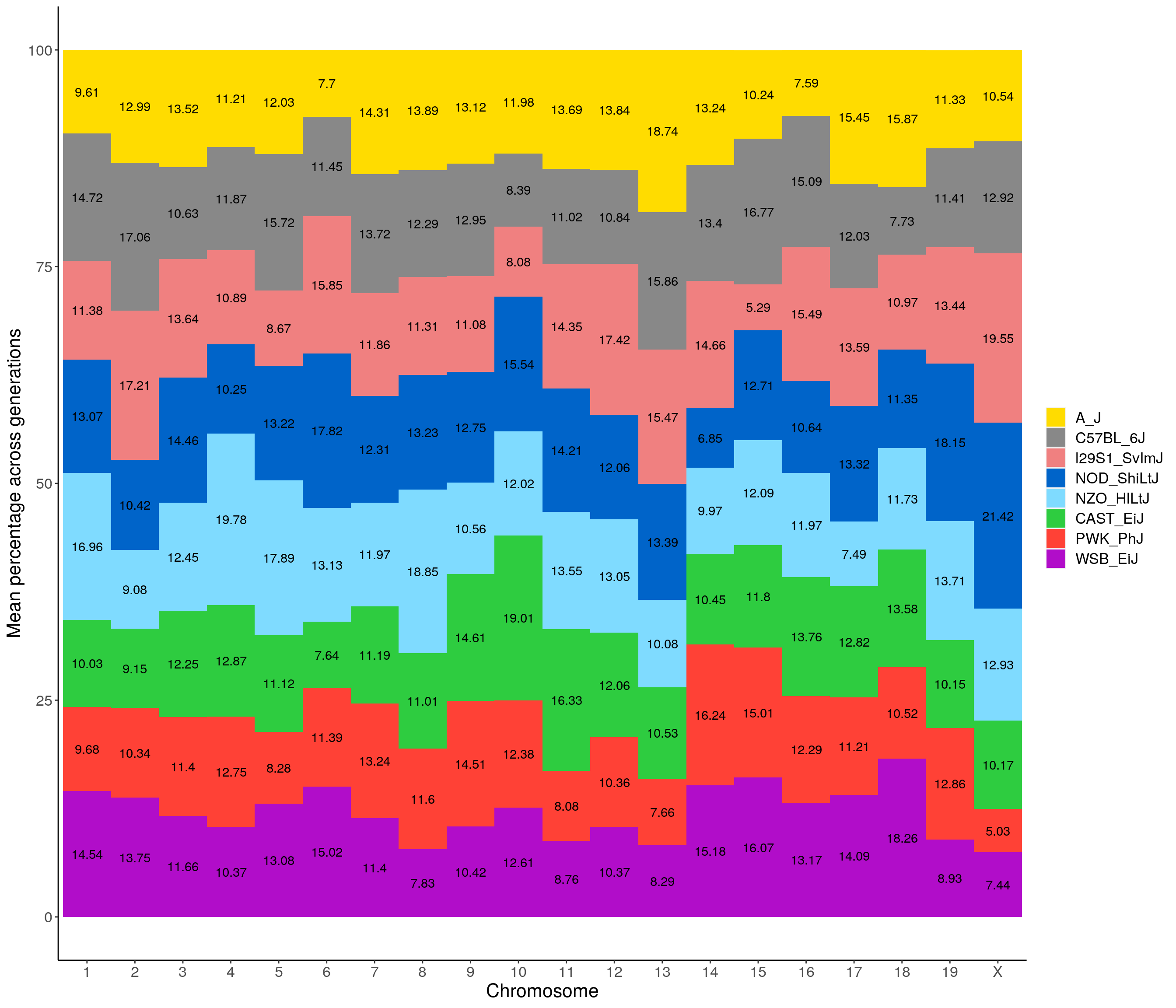
#Stackbar plot
#summarize per chromosome across generation
pdf(file = "data/Jackson_Lab_12_batches/stackbar_mean_prop_across_all_chr.pdf",width = 16)
p02 <- fp %>% group_by(gen, founder) %>%
  summarise(grand_mean = round(100*mean(prop), 2),
            grand_sd   = round(100*sd(prop), 2)) %>%
  ggplot(aes(x = gen, y = grand_mean, fill = founder)) +
    geom_bar(stat="identity",
             width=0.99) +
    geom_text(aes(label = paste0(grand_mean, " ± ", grand_sd)), position = position_stack(vjust = 0.5)) +
    scale_fill_manual(values = CCcolors) +
    ylab("Mean percentage across all chromosomes") +
    xlab("Generation") +
    theme(panel.grid.major = element_blank(),
          panel.grid.minor = element_blank(),
          panel.background = element_blank(),
          axis.line = element_line(colour = "black"),
          plot.title = element_text(hjust = 0.5),
          text = element_text(size=16),
          axis.title=element_text(size=16),
          legend.title=element_blank())
`summarise()` regrouping output by 'gen' (override with `.groups` argument)p02
dev.off()png
2 p02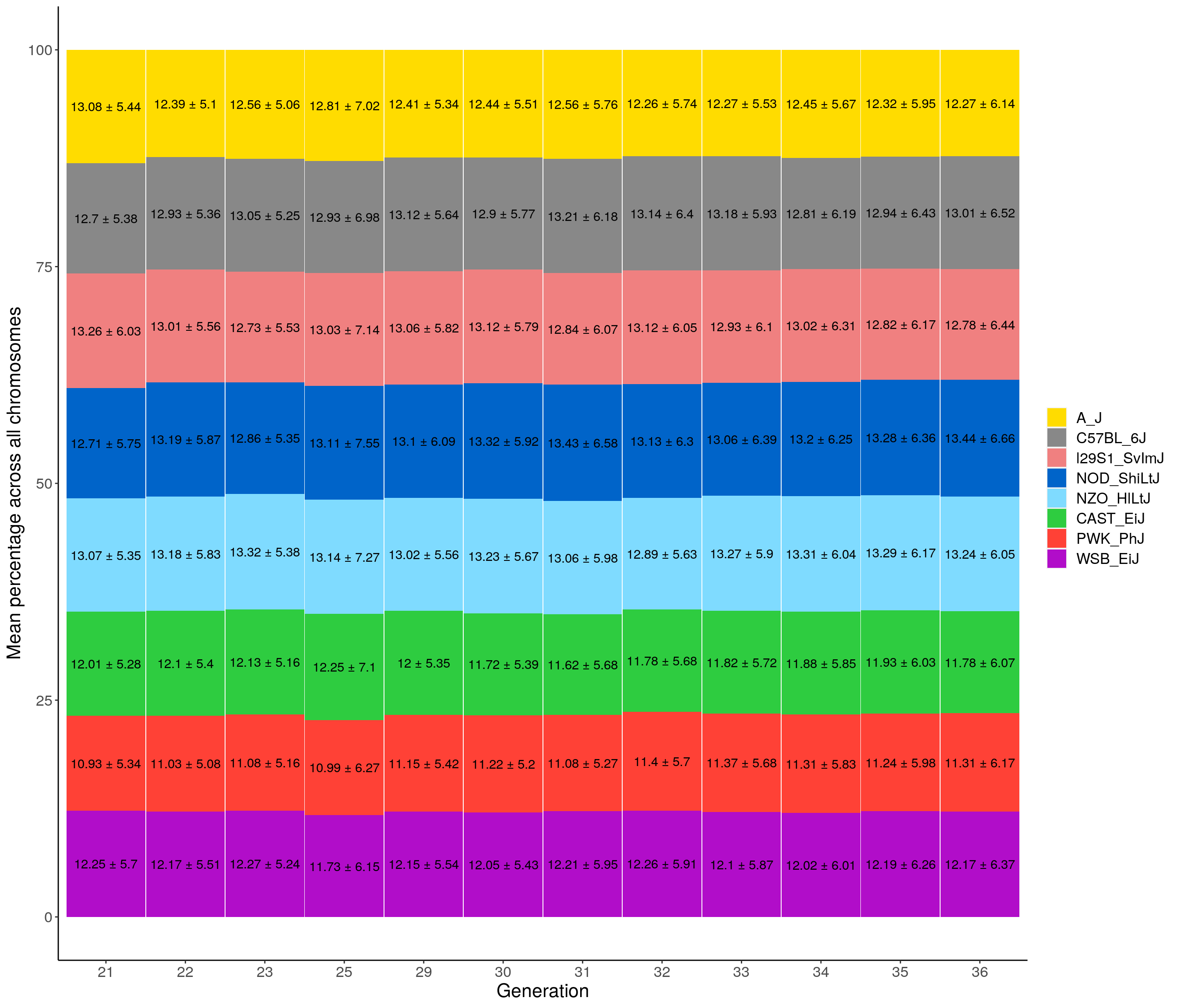
#stackbar_prop_across_gen
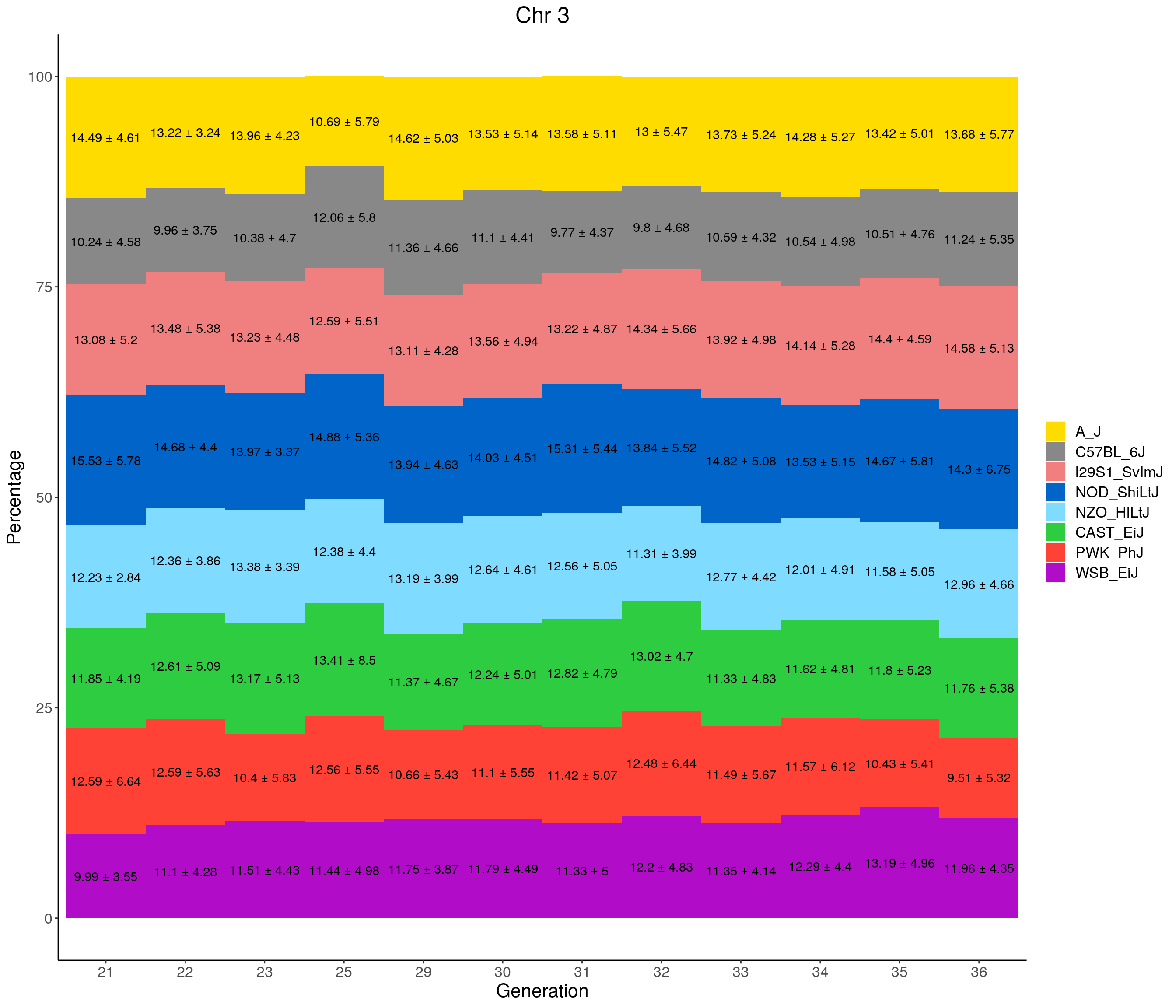
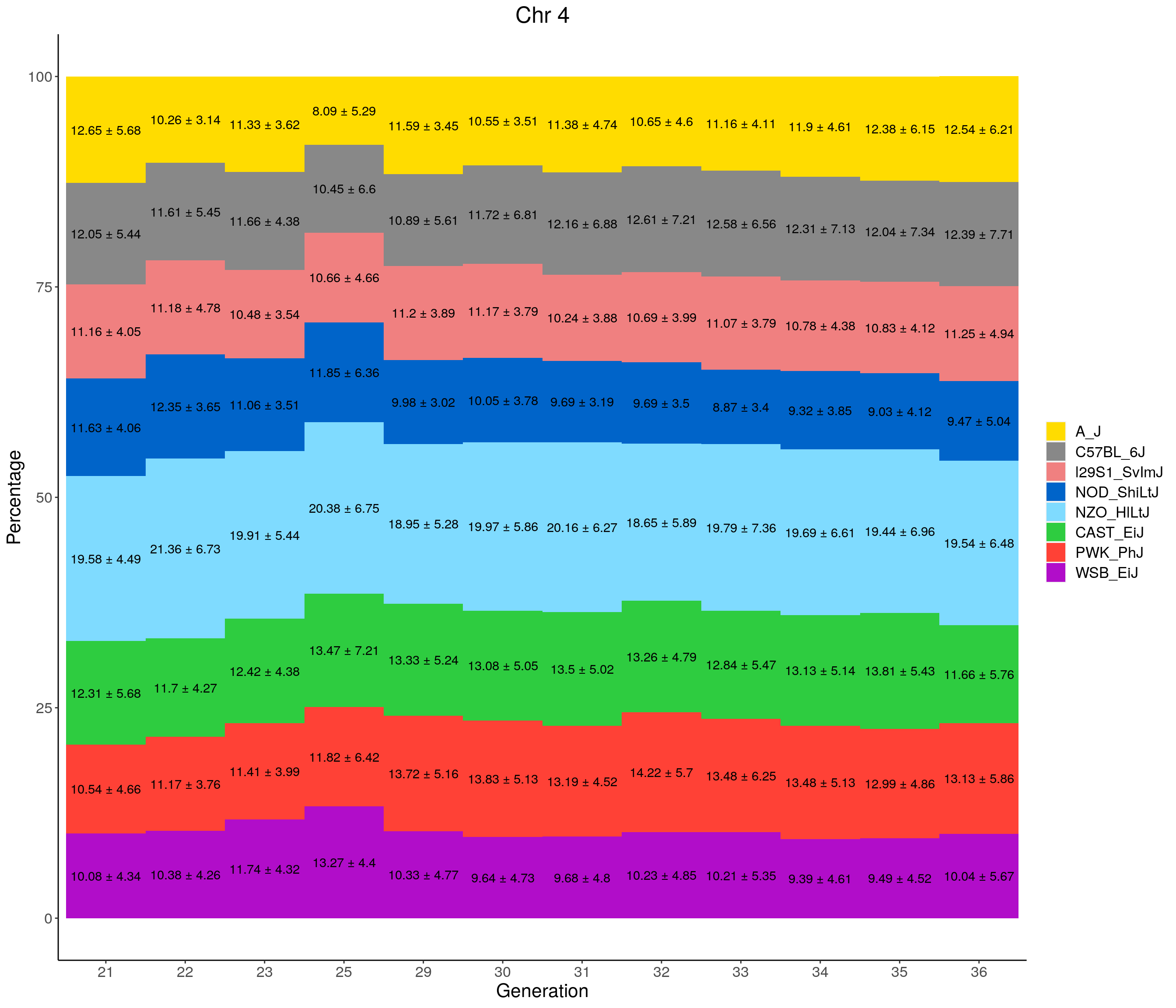
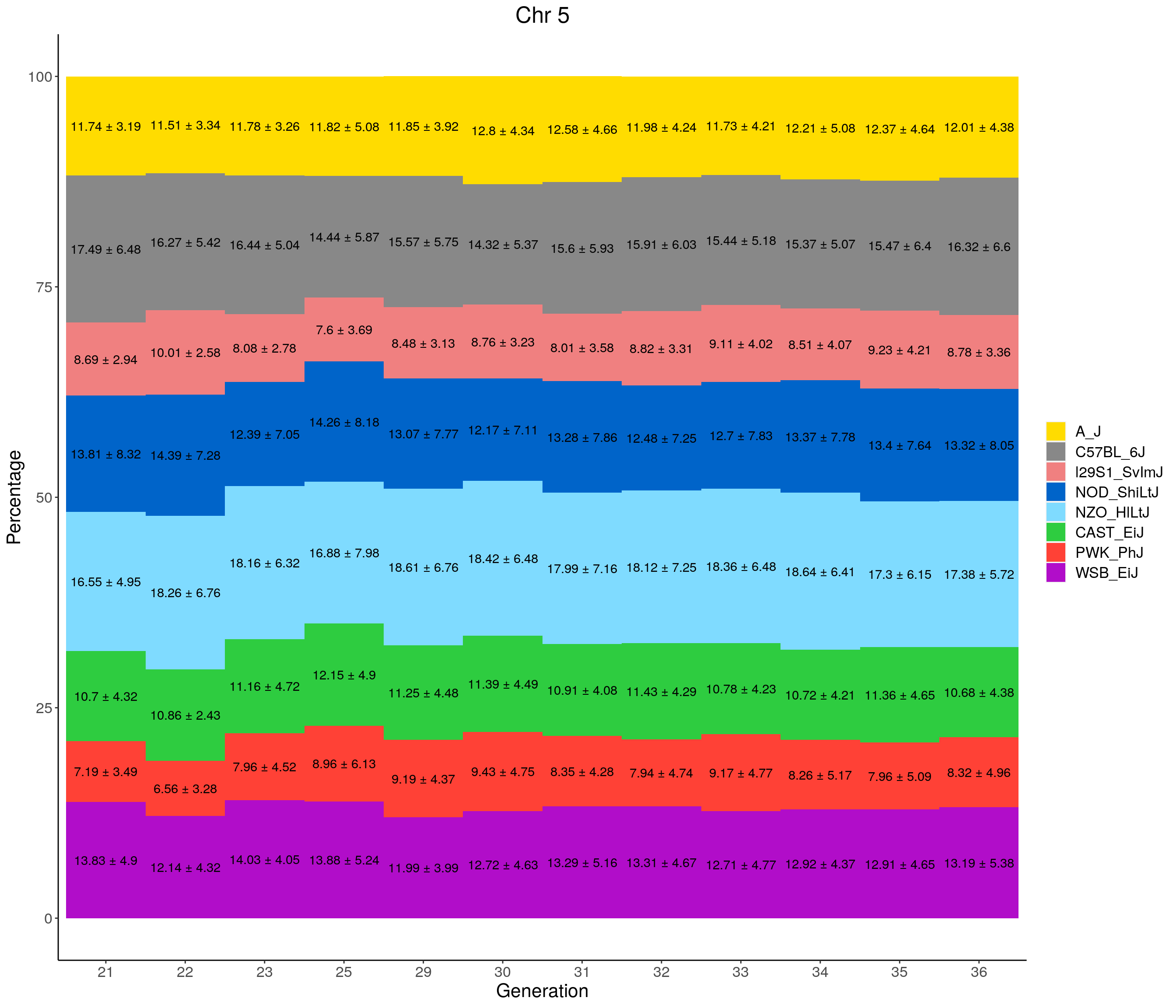
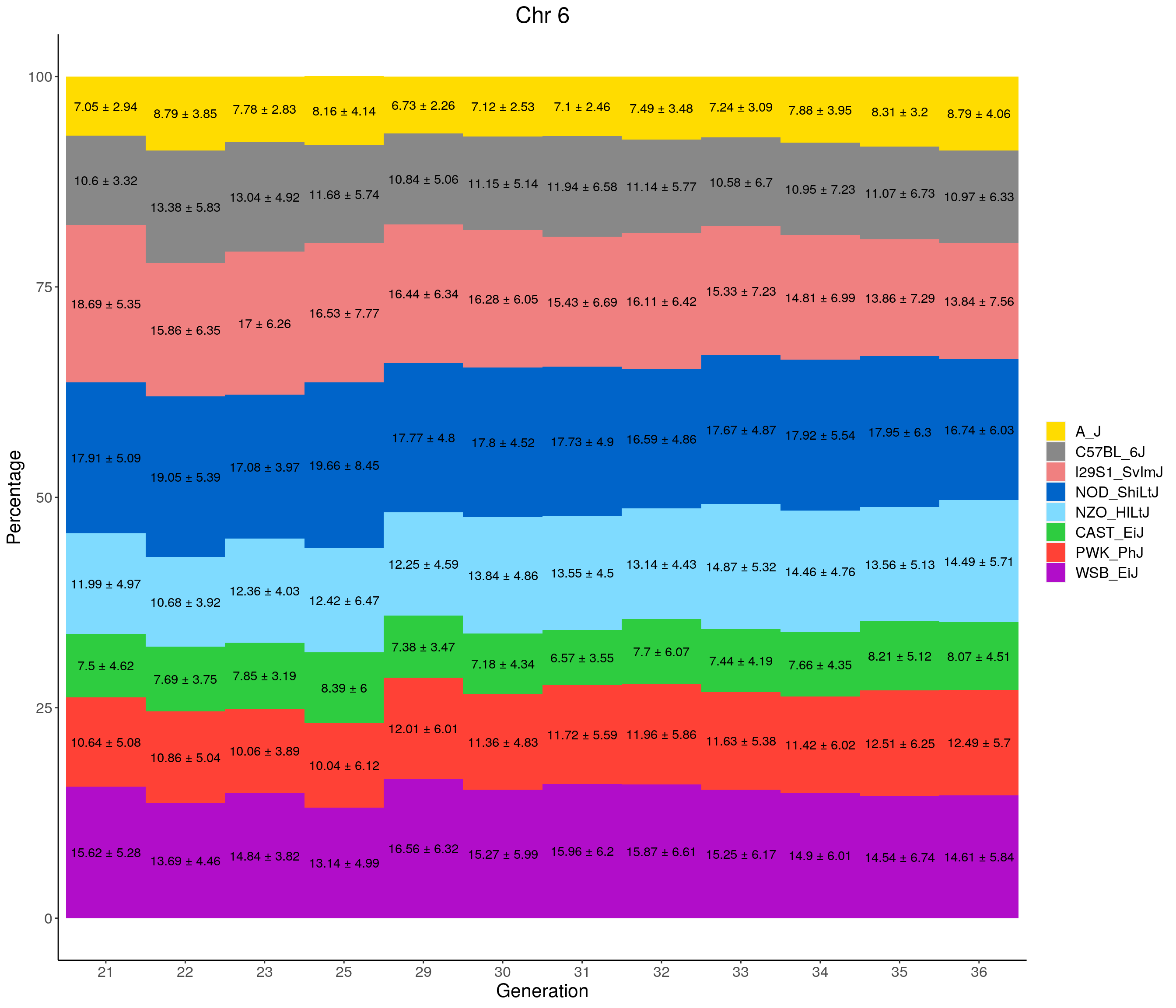
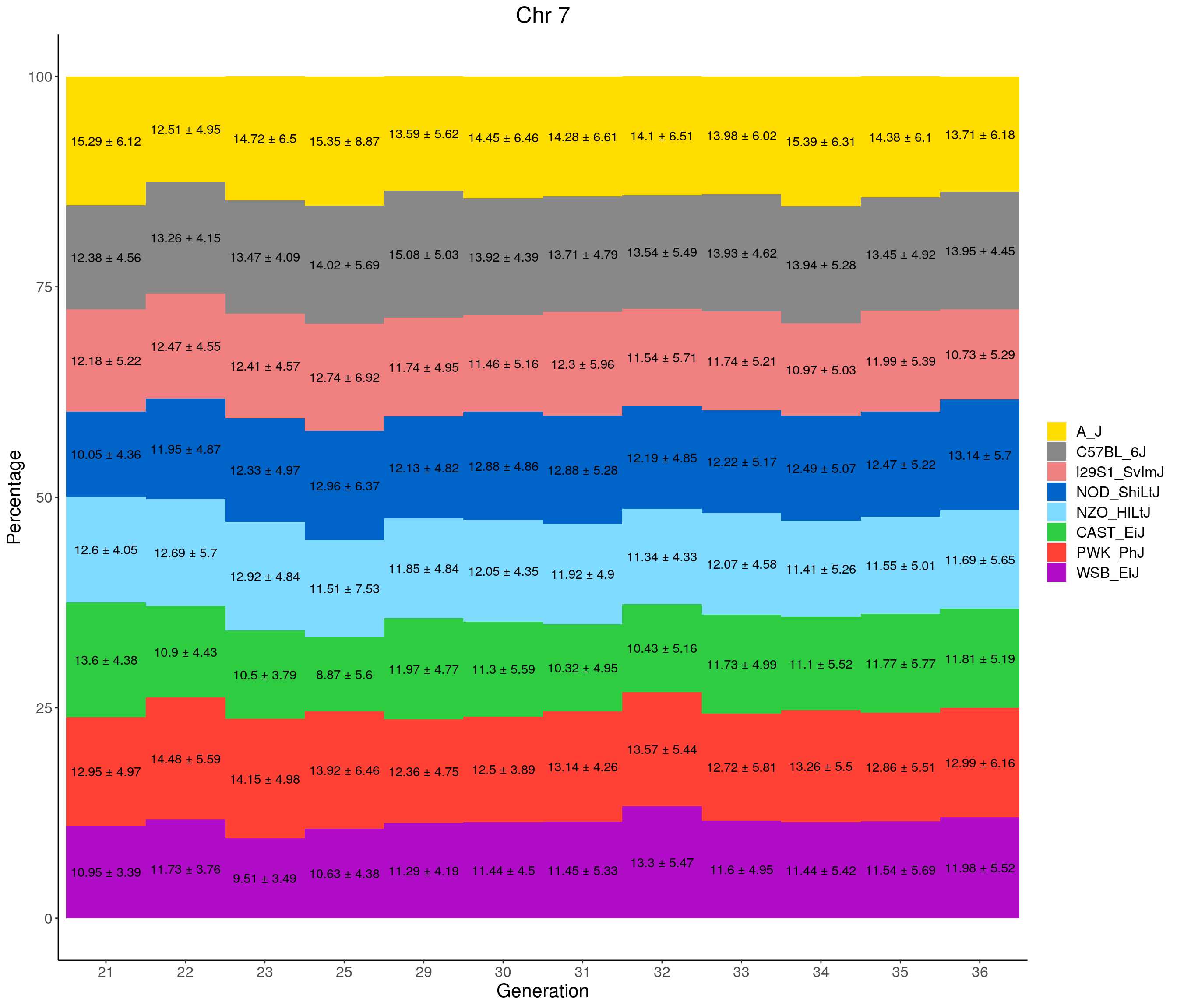
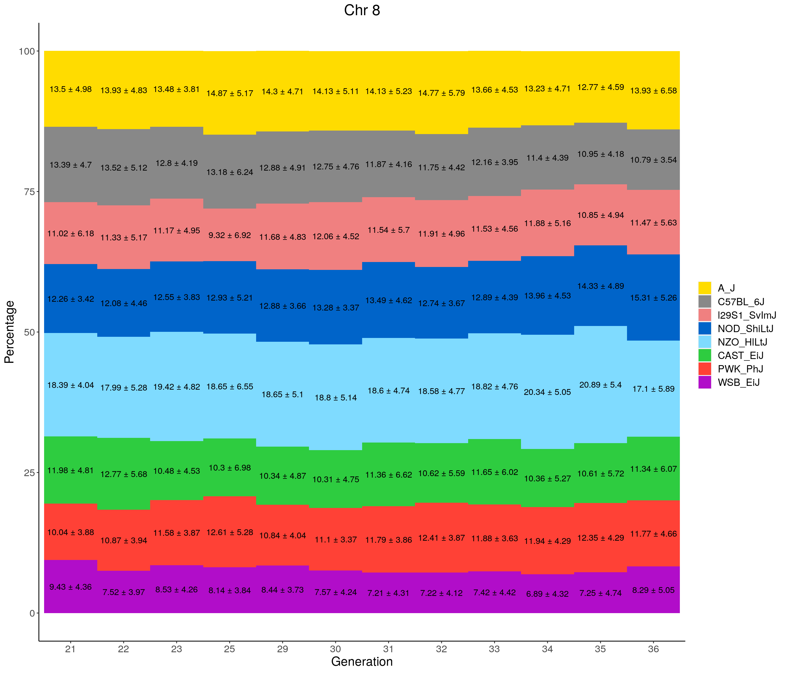
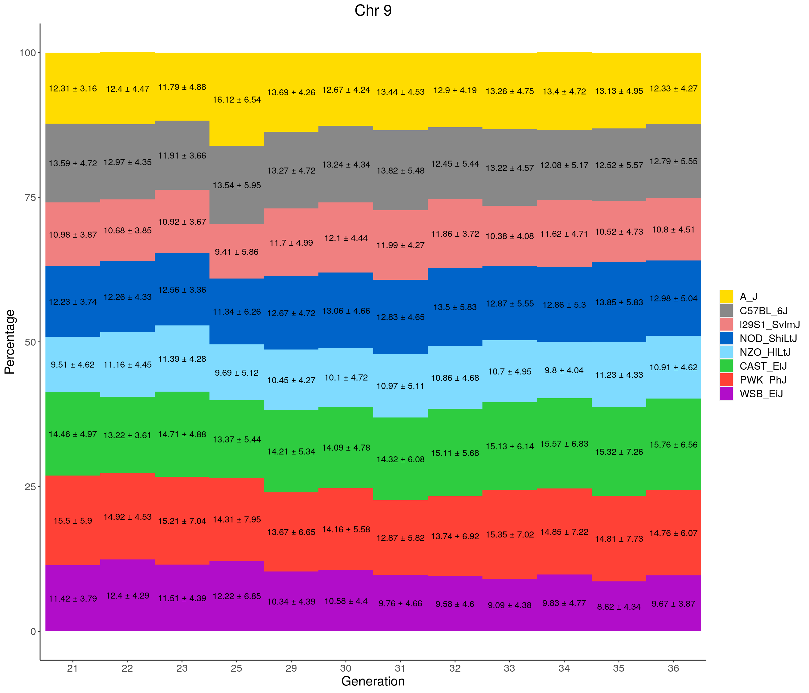
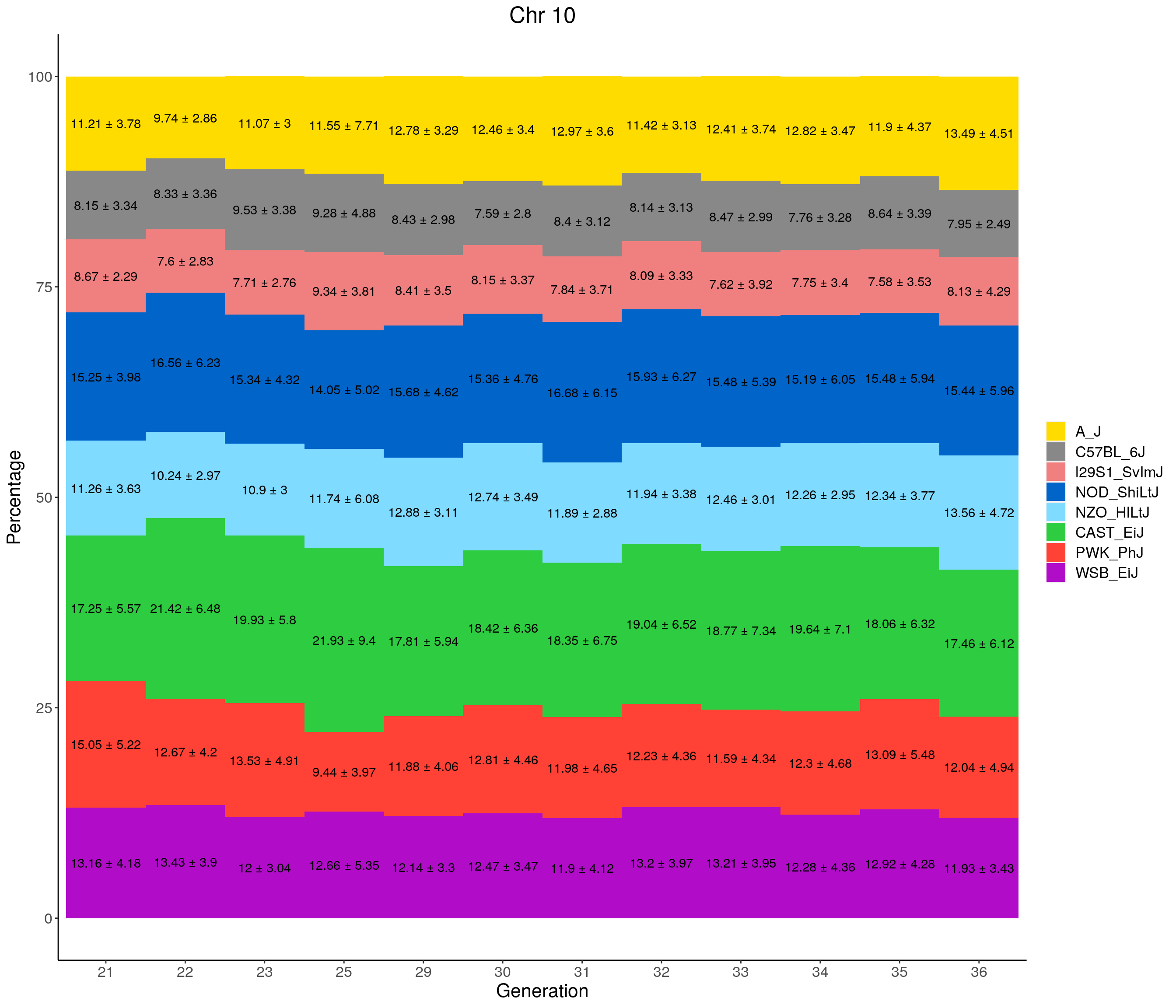
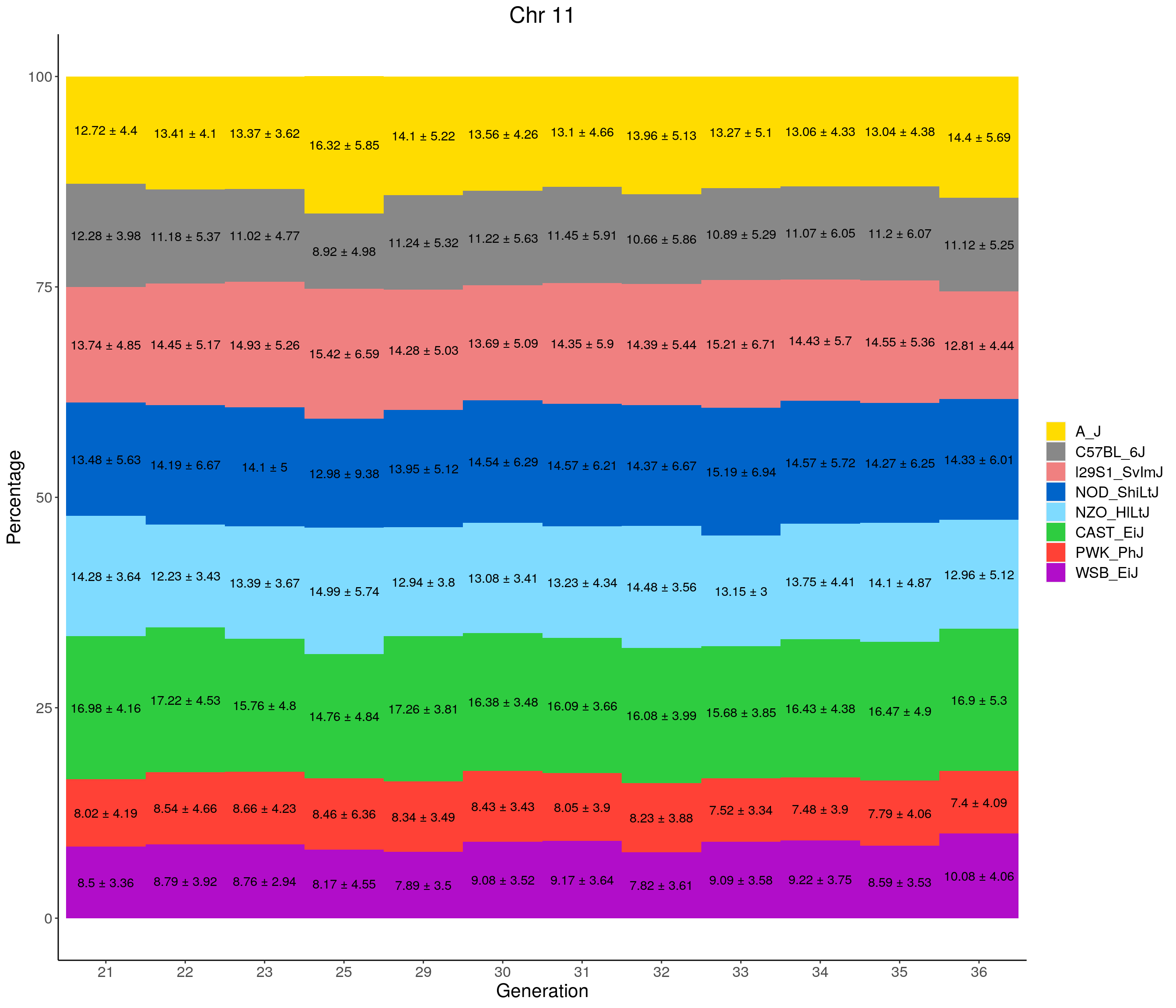
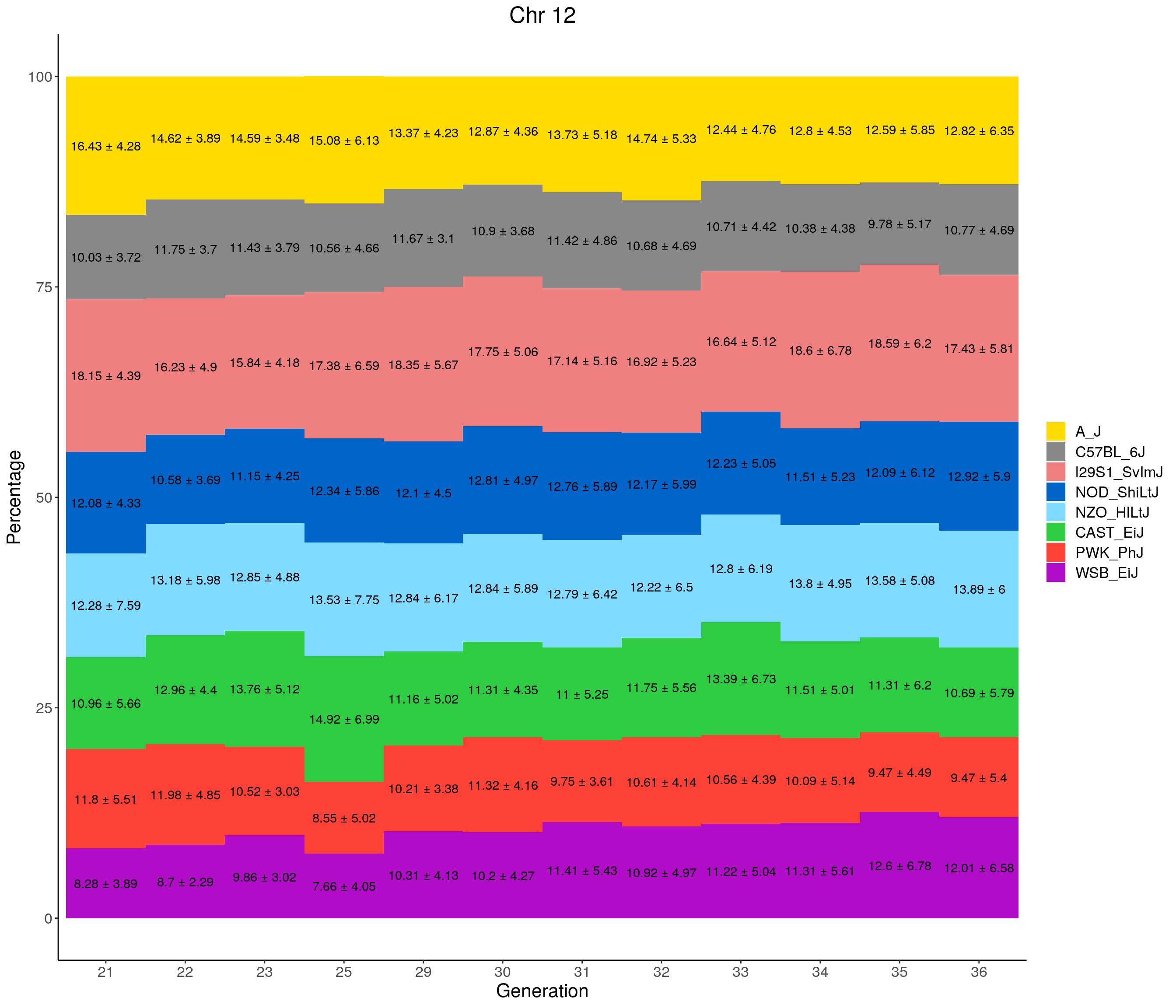
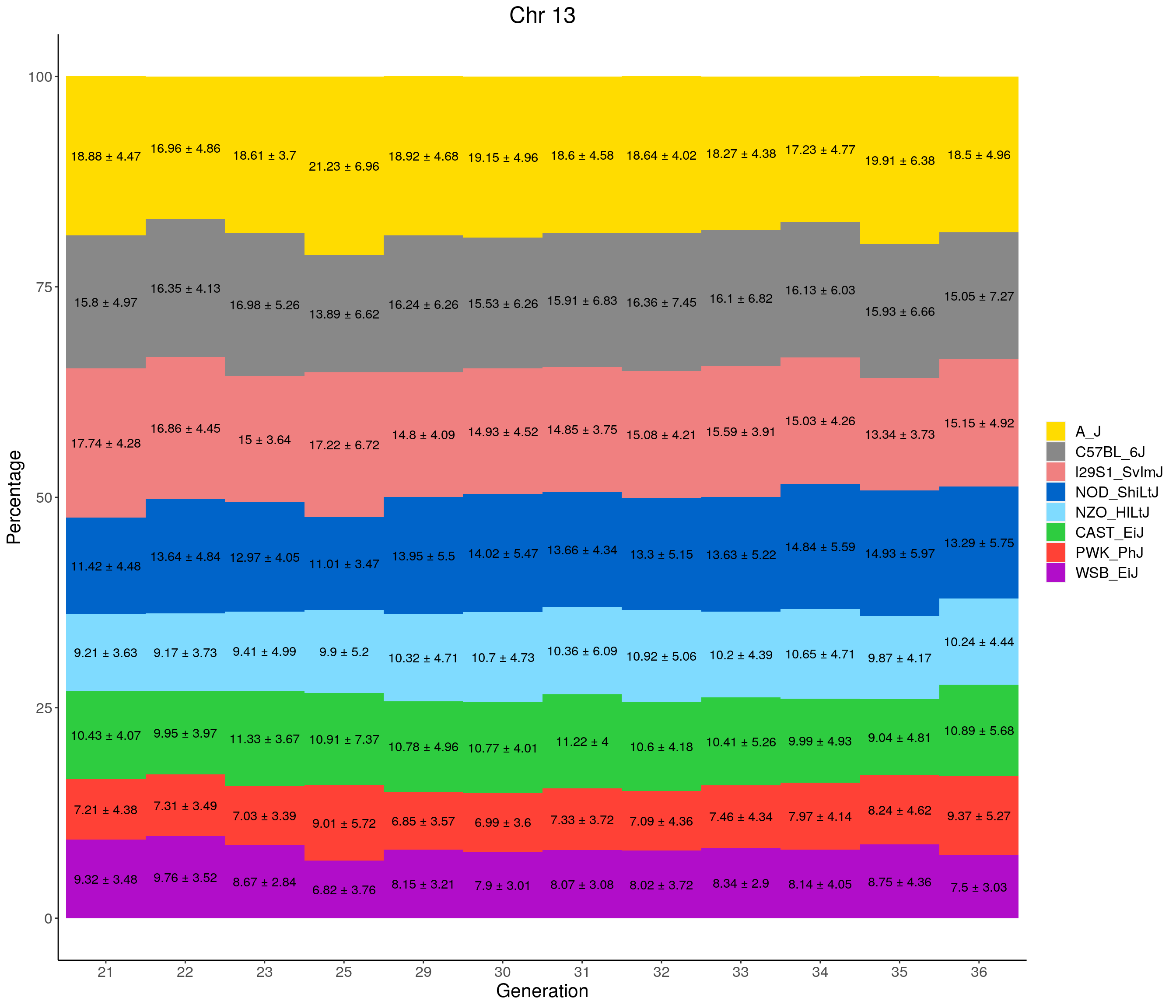
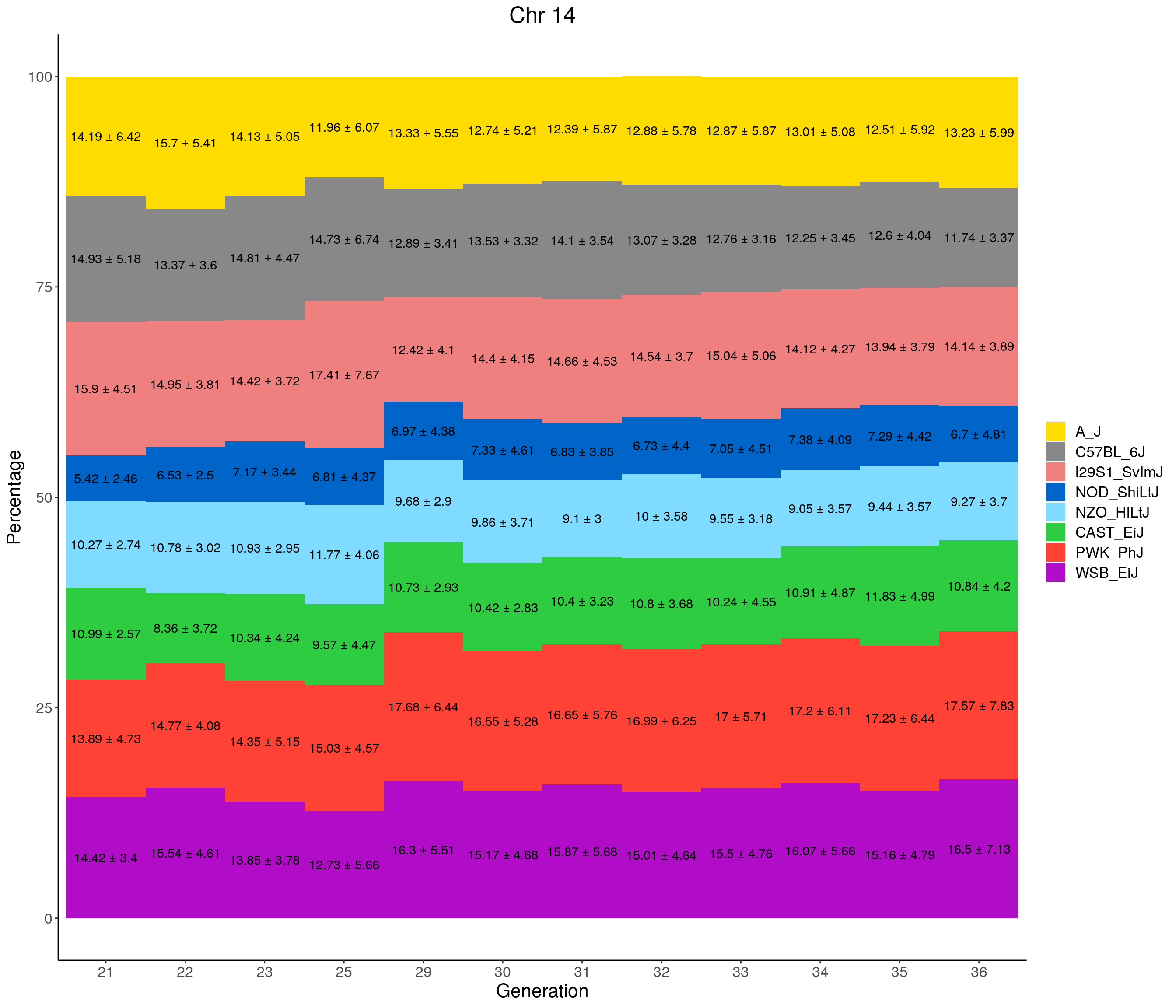
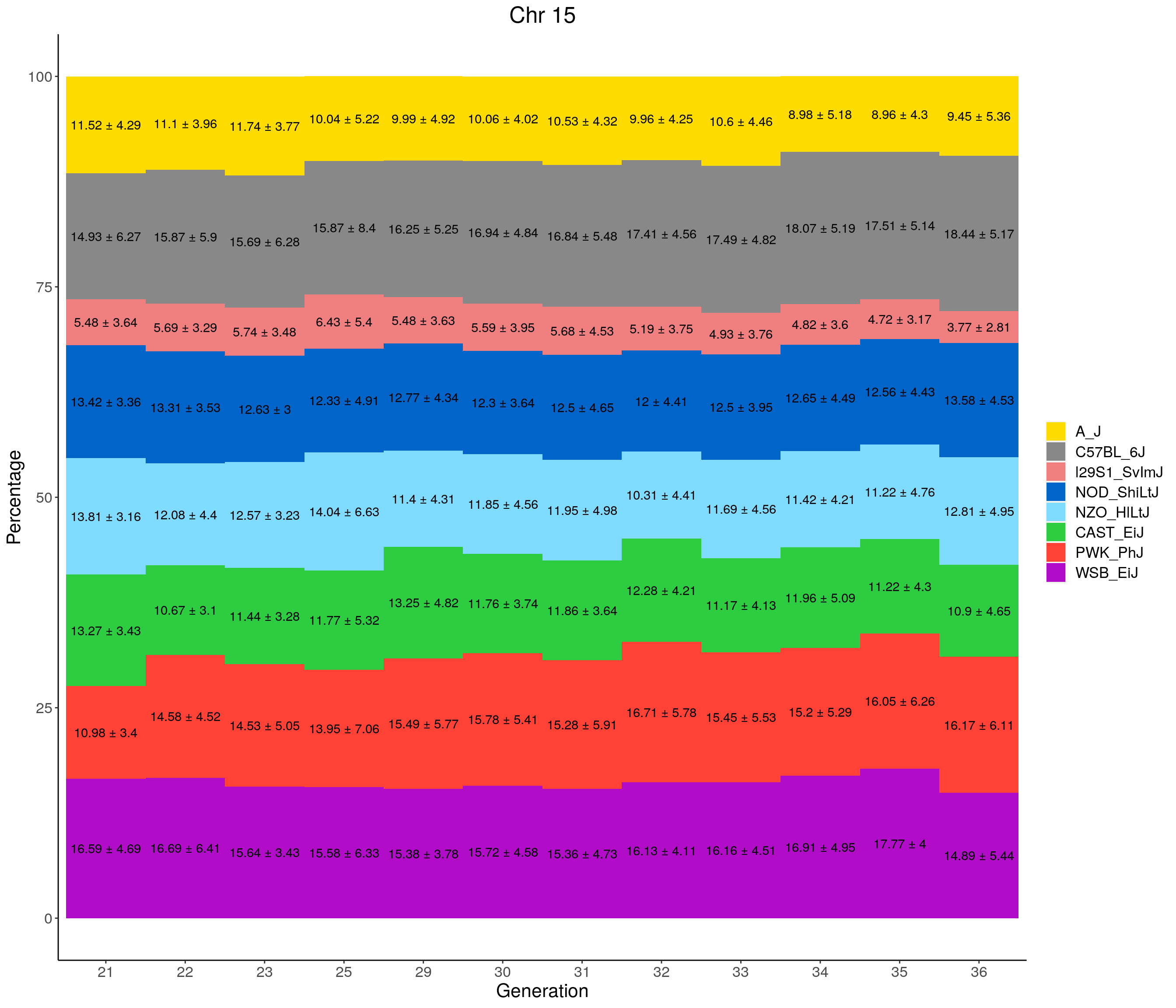
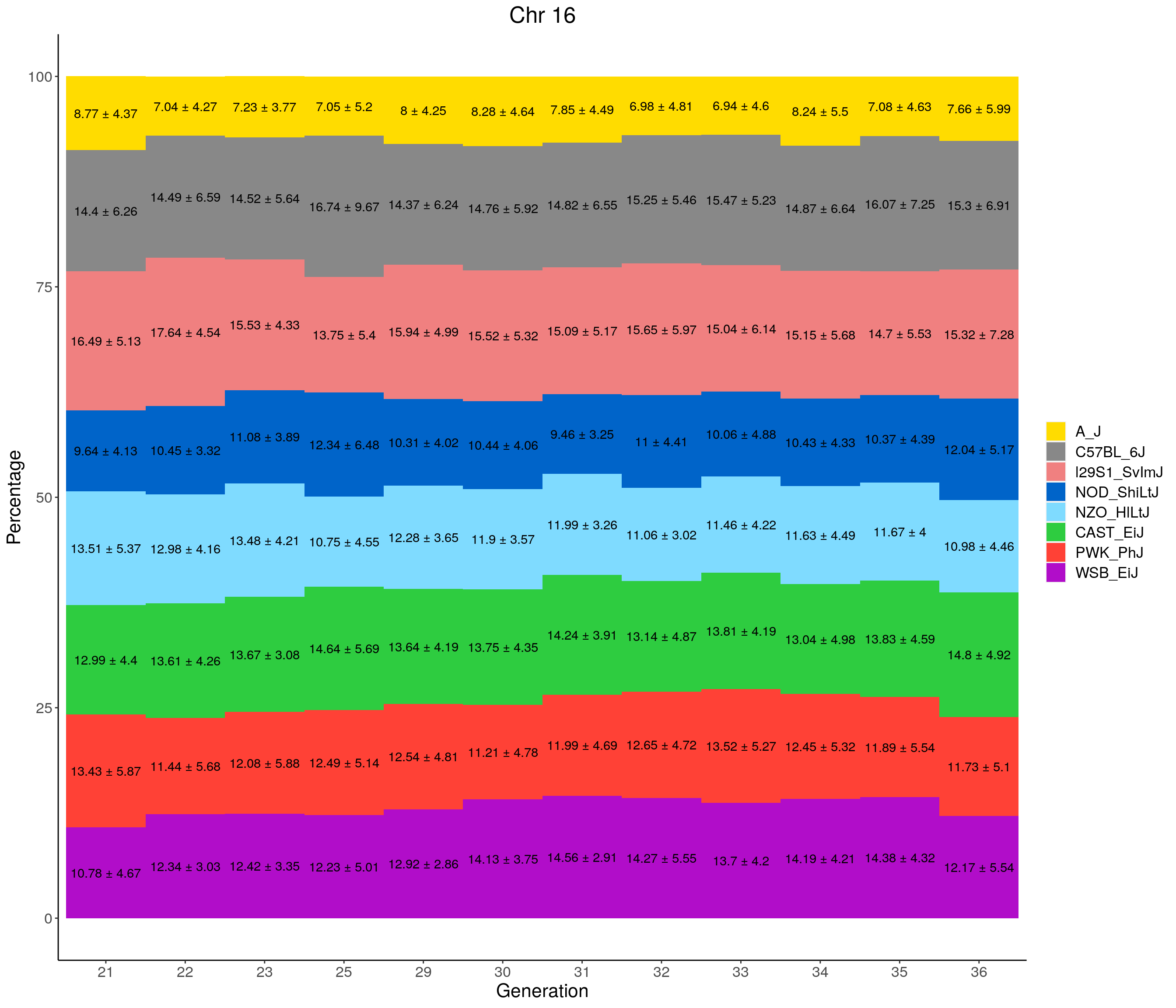
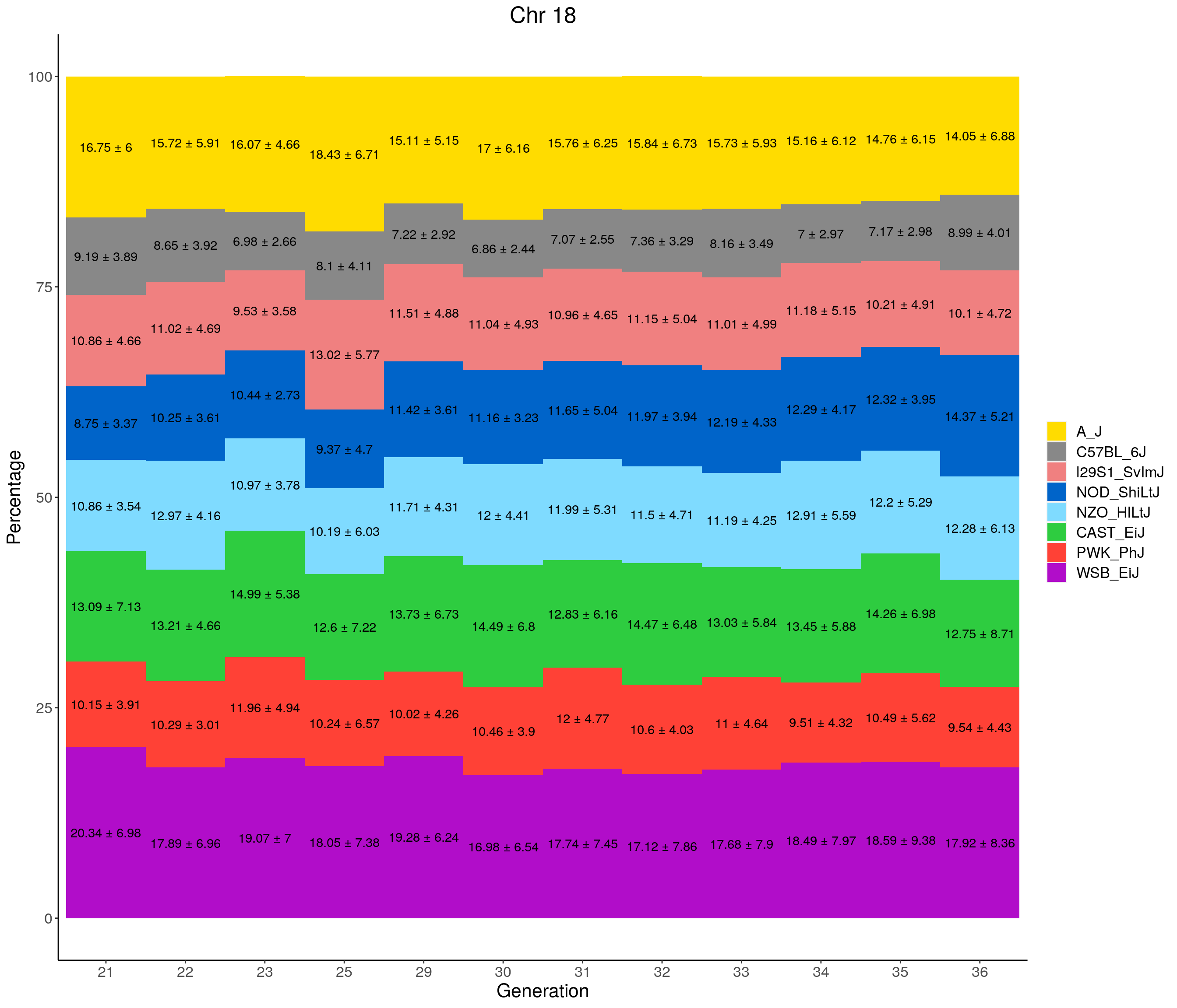
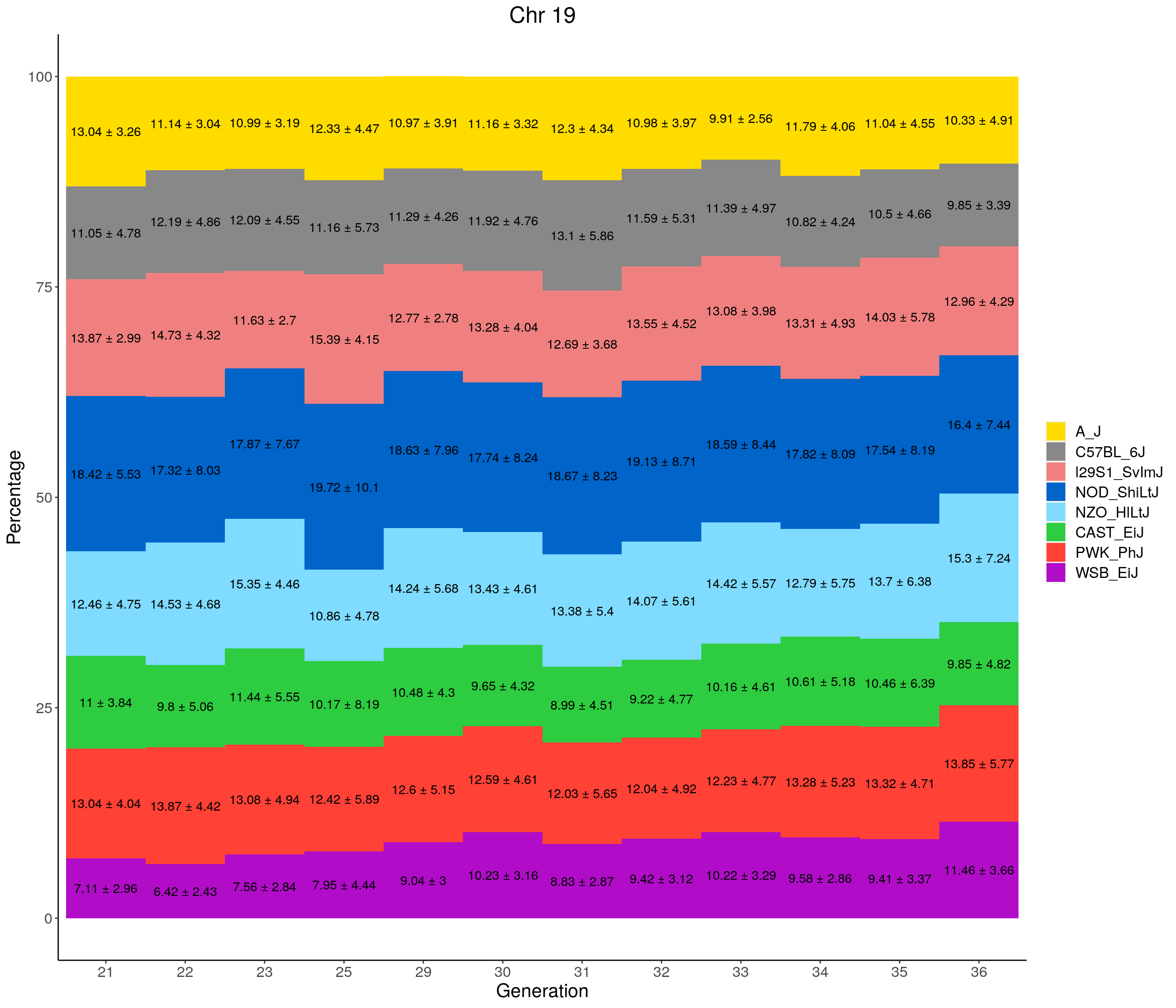
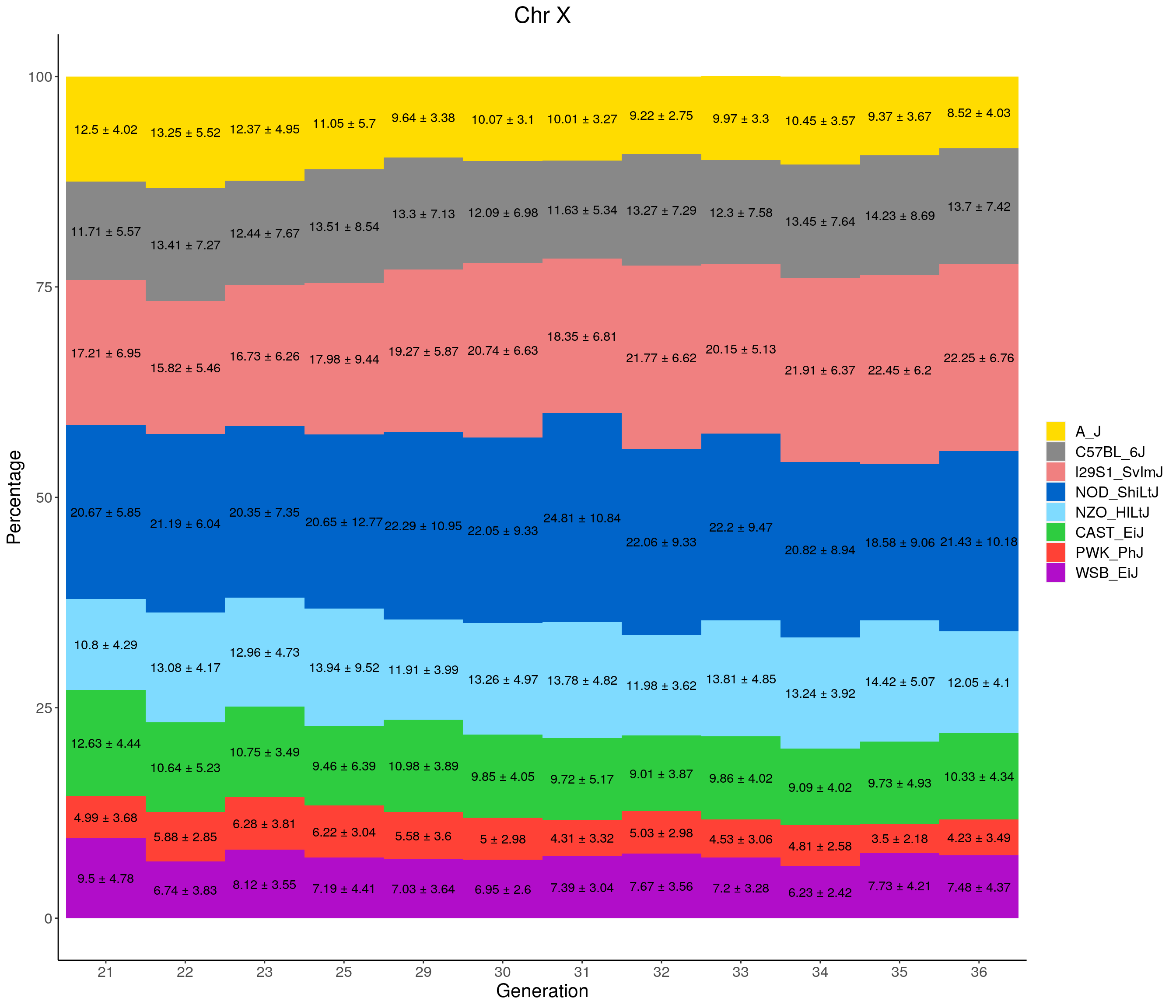
for(c in c(1:19, "X")){
#print(c)
p <- ggplot(data = fp_summary[fp_summary$chr == c,], aes(x = gen, y = mean, fill = founder)) +
geom_bar(stat="identity",
width=1) +
geom_text(aes(label = paste0(mean," ± ", sd)), position = position_stack(vjust = 0.5)) +
scale_fill_manual(values = CCcolors) +
labs(title = paste0("Chr ", c)) +
ylab("Percentage") +
xlab("Generation") +
theme(panel.grid.major = element_blank(),
panel.grid.minor = element_blank(),
panel.background = element_blank(),
axis.line = element_line(colour = "black"),
plot.title = element_text(hjust = 0.5),
text = element_text(size=16),
axis.title=element_text(size=16),
legend.title=element_blank())
print(p)
}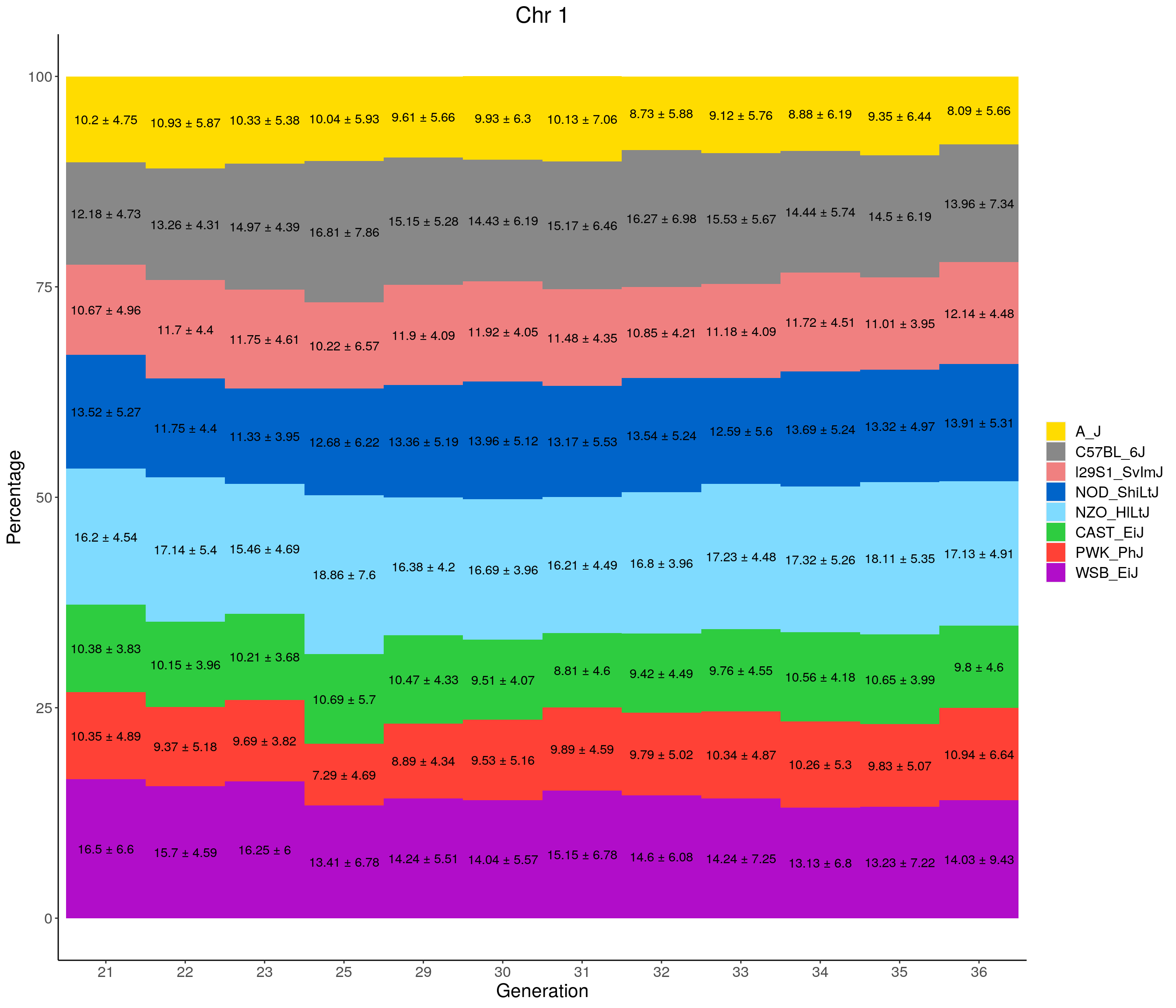
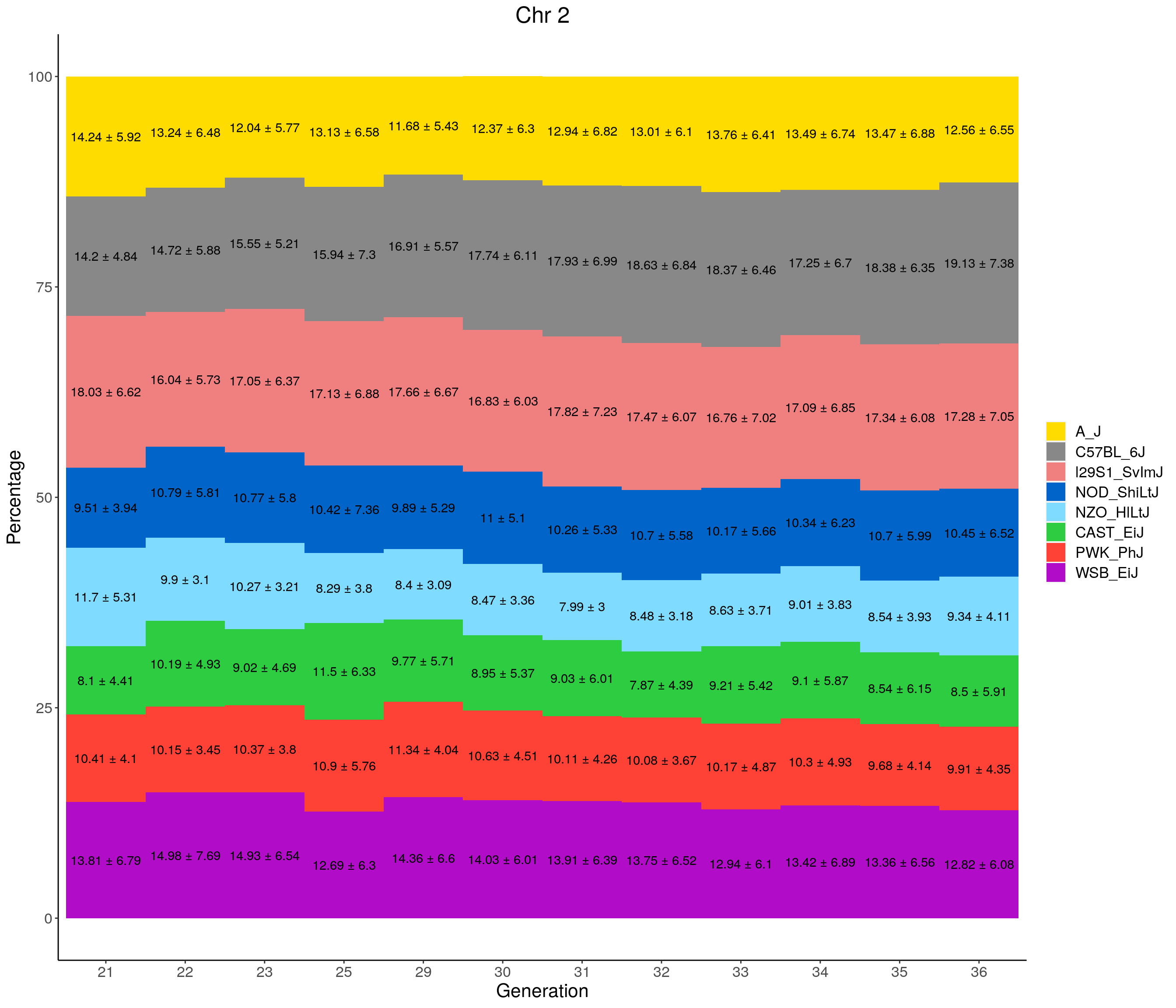

pdf(file = "data/Jackson_Lab_12_batches/stackbar_prop_across_gen.pdf",width = 16)
for(c in c(1:19, "X")){
  #print(c)
  p <- ggplot(data = fp_summary[fp_summary$chr == c,], aes(x = gen, y = mean, fill = founder)) +
    geom_bar(stat="identity",
             width=1) +
    geom_text(aes(label = paste0(mean," ± ", sd)), position = position_stack(vjust = 0.5)) +
    scale_fill_manual(values = CCcolors) +
    labs(title = paste0("Chr ", c)) +
    ylab("Percentage") +
    xlab("Generation") +
    theme(panel.grid.major = element_blank(),
          panel.grid.minor = element_blank(),
          panel.background = element_blank(),
          axis.line = element_line(colour = "black"),
          plot.title = element_text(hjust = 0.5),
          text = element_text(size=16),
          axis.title=element_text(size=16),
          legend.title=element_blank())
  print(p)
}
dev.off()
png
2 #stackbar_prop_across_chr
for(g in levels(fp_summary$gen)){
#print(g)
p <- ggplot(data = fp_summary[fp_summary$gen == g,], aes(x = chr, y = mean, fill = founder)) +
geom_bar(stat="identity",
width=1) +
geom_text(aes(label = paste0(mean)), position = position_stack(vjust = 0.5)) +
scale_fill_manual(values = CCcolors) +
labs(title = paste0("Generation ", g)) +
ylab("Percentage") +
theme(panel.grid.major = element_blank(),
panel.grid.minor = element_blank(),
panel.background = element_blank(),
axis.title.x = element_blank(),
axis.line = element_line(colour = "black"),
plot.title = element_text(hjust = 0.5),
text = element_text(size=16),
axis.title=element_text(size=16),
legend.title=element_blank())
#print(p)
}
pdf(file = "data/Jackson_Lab_12_batches/stackbar_prop_across_chr.pdf", width = 12)
for(g in levels(fp_summary$gen)){
#print(g)
p <- ggplot(data = fp_summary[fp_summary$gen == g,], aes(x = chr, y = mean, fill = founder)) +
geom_bar(stat="identity",
width=1) +
geom_text(aes(label = paste0(mean)), position = position_stack(vjust = 0.5)) +
scale_fill_manual(values = CCcolors) +
labs(title = paste0("Generation ", g)) +
ylab("Percentage") +
theme(panel.grid.major = element_blank(),
panel.grid.minor = element_blank(),
panel.background = element_blank(),
axis.title.x = element_blank(),
axis.line = element_line(colour = "black"),
plot.title = element_text(hjust = 0.5),
text = element_text(size=16),
axis.title=element_text(size=16),
legend.title=element_blank())
print(p)
}
dev.off()png
2 #line plot
#plt <- htmltools::tagList()
for(c in unique(names(gm_after_qc$geno))){
print(c)
fp_subdata <- fp[fp$chr == c,]
pp <- ggplot(data = fp_subdata,aes(pos, prop, group = gen, color = founder)) +
geom_line(aes(linetype=gen)) +
scale_linetype_manual(values=rep("solid",12)) +
geom_hline(yintercept=0.125, linetype="dashed", color = "black", size = 0.25) +
scale_color_manual(values = CCcolors) +
facet_grid(founder~.) +
labs(title = paste0("Chr ", c)) +
theme(legend.position='none')
print(pp)
# Print an interactive plot
# Add to list
#plt[[c]] <- as_widget(ggplotly(pp, width = 1000, height = 1000))
}[1] "1"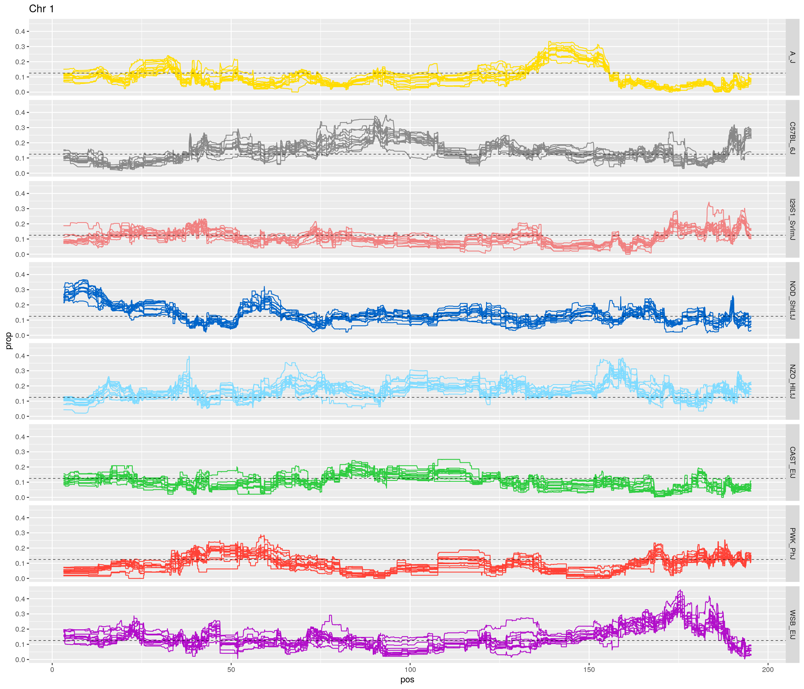
[1] "2"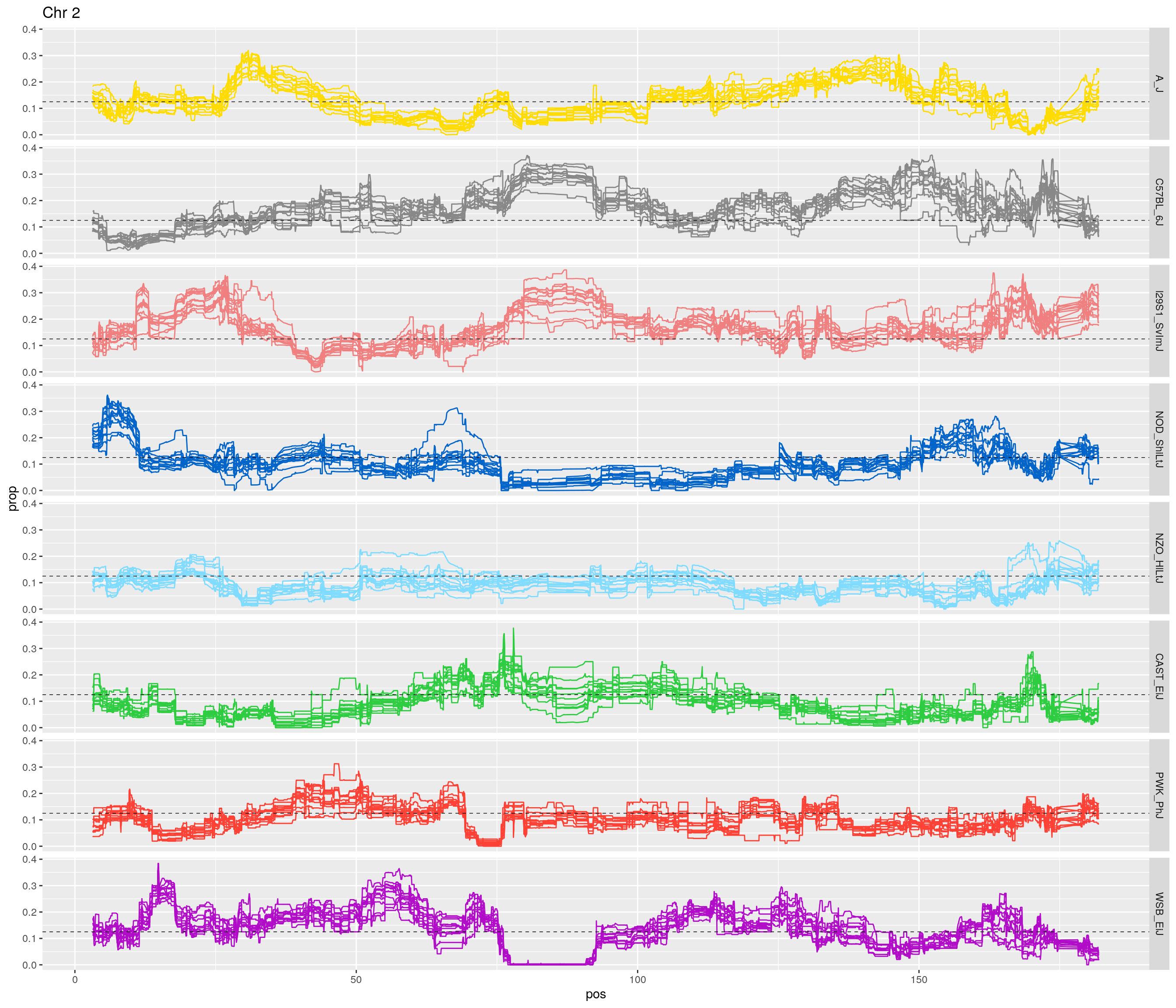
[1] "3"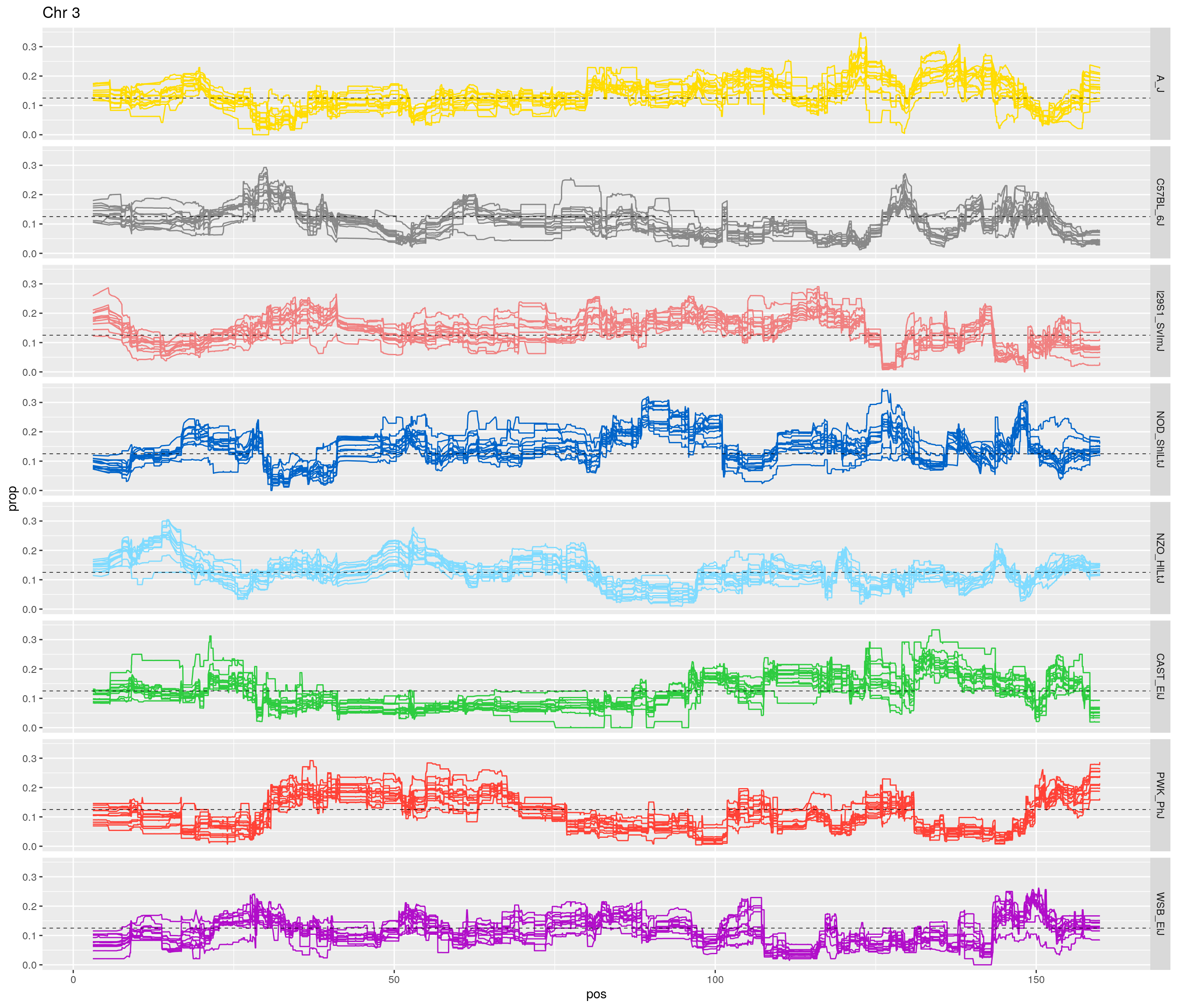
[1] "4"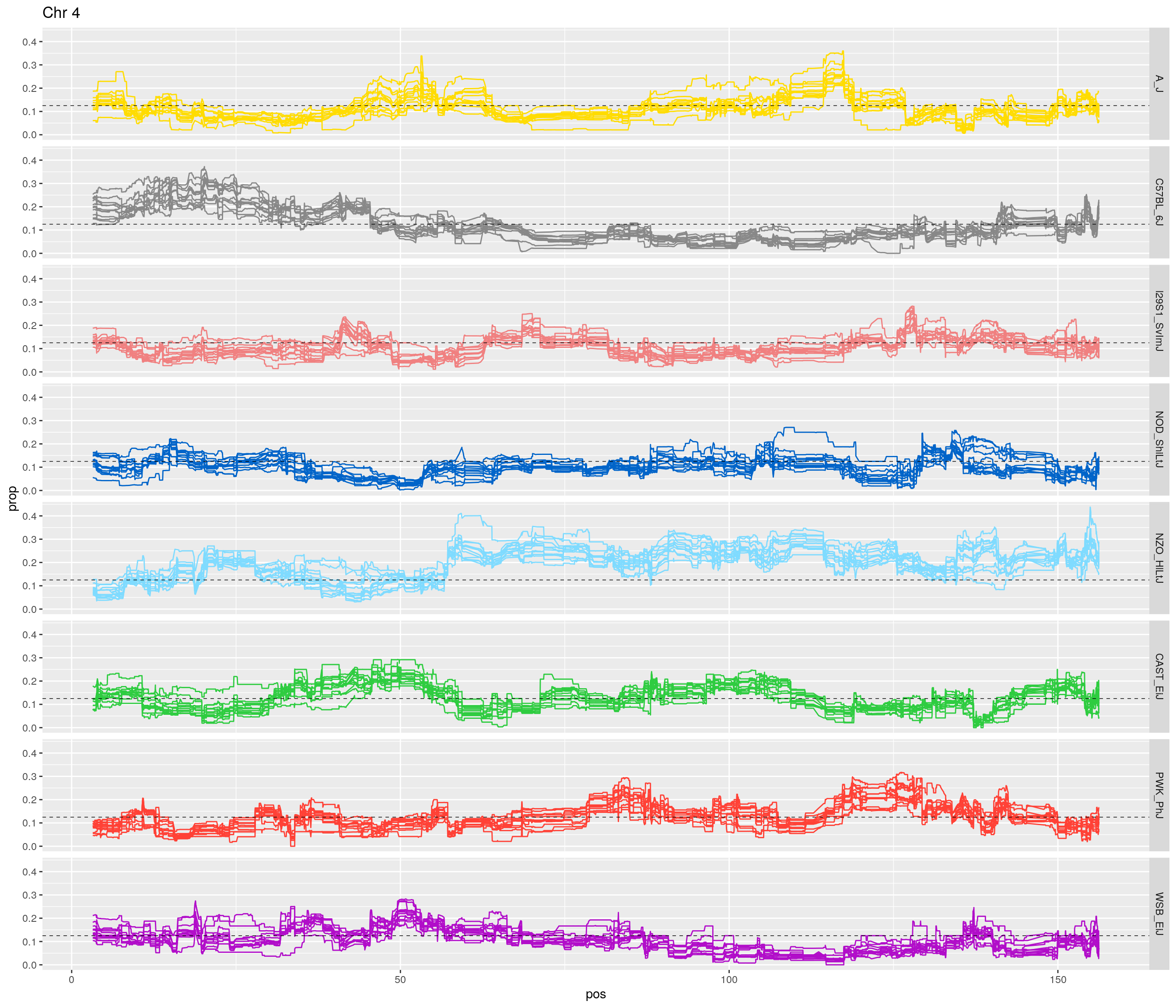
[1] "5"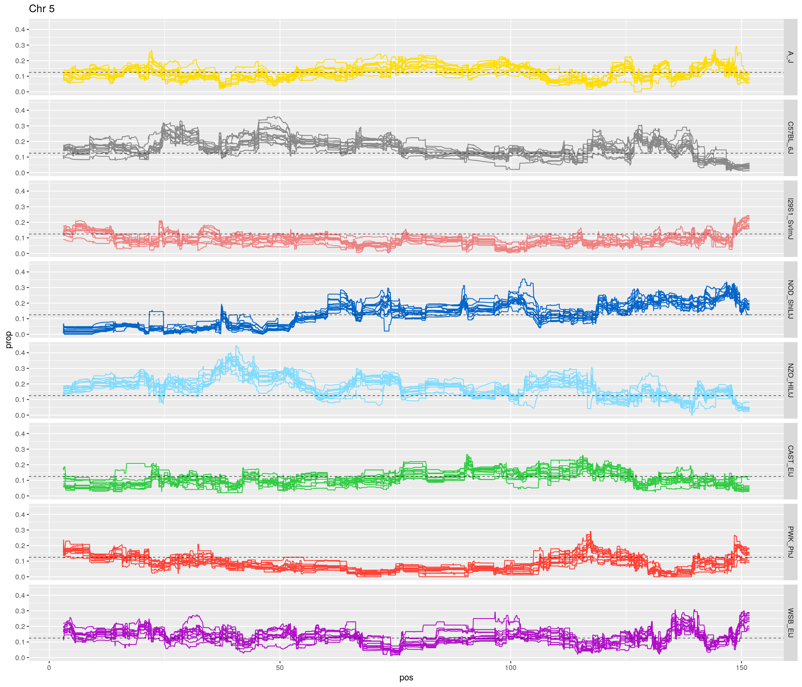
[1] "6"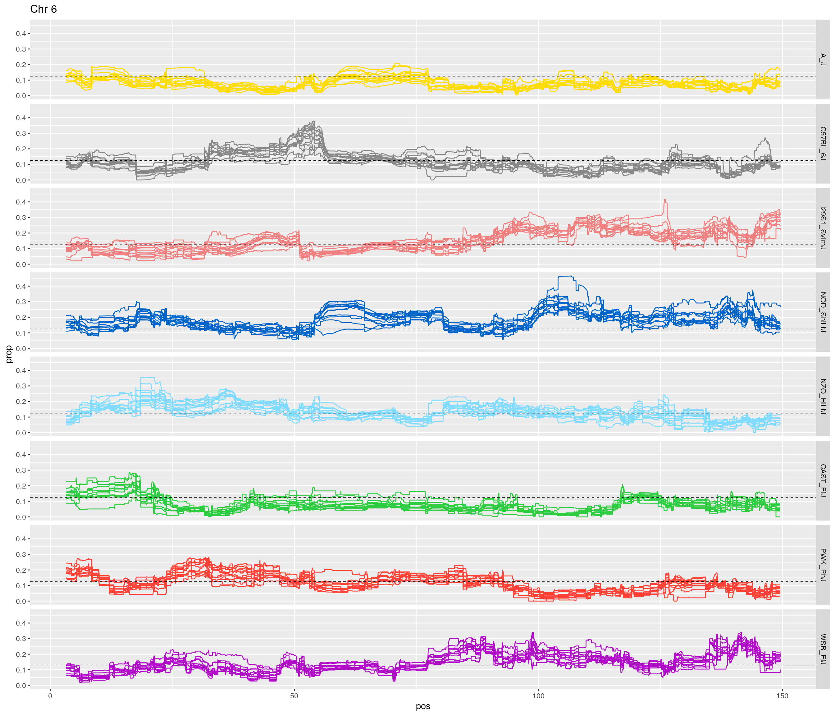
[1] "7"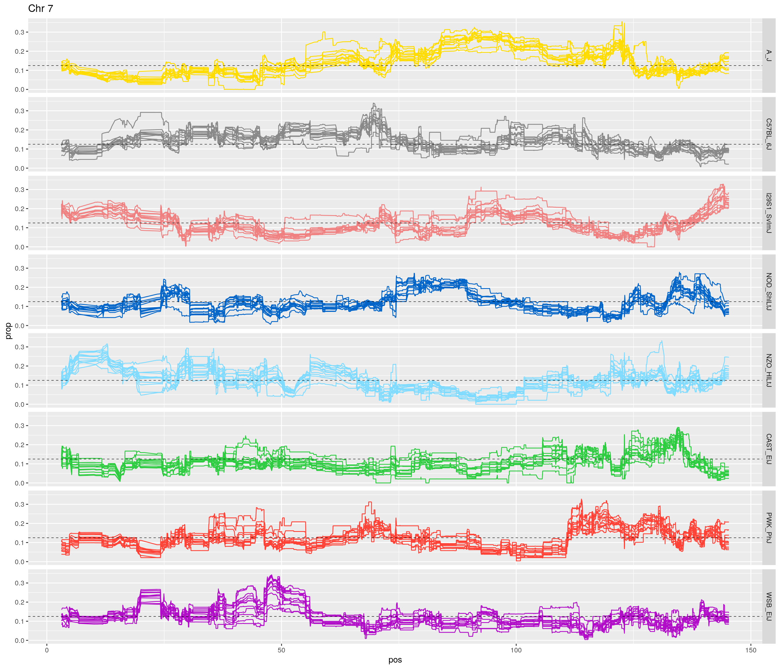
[1] "8"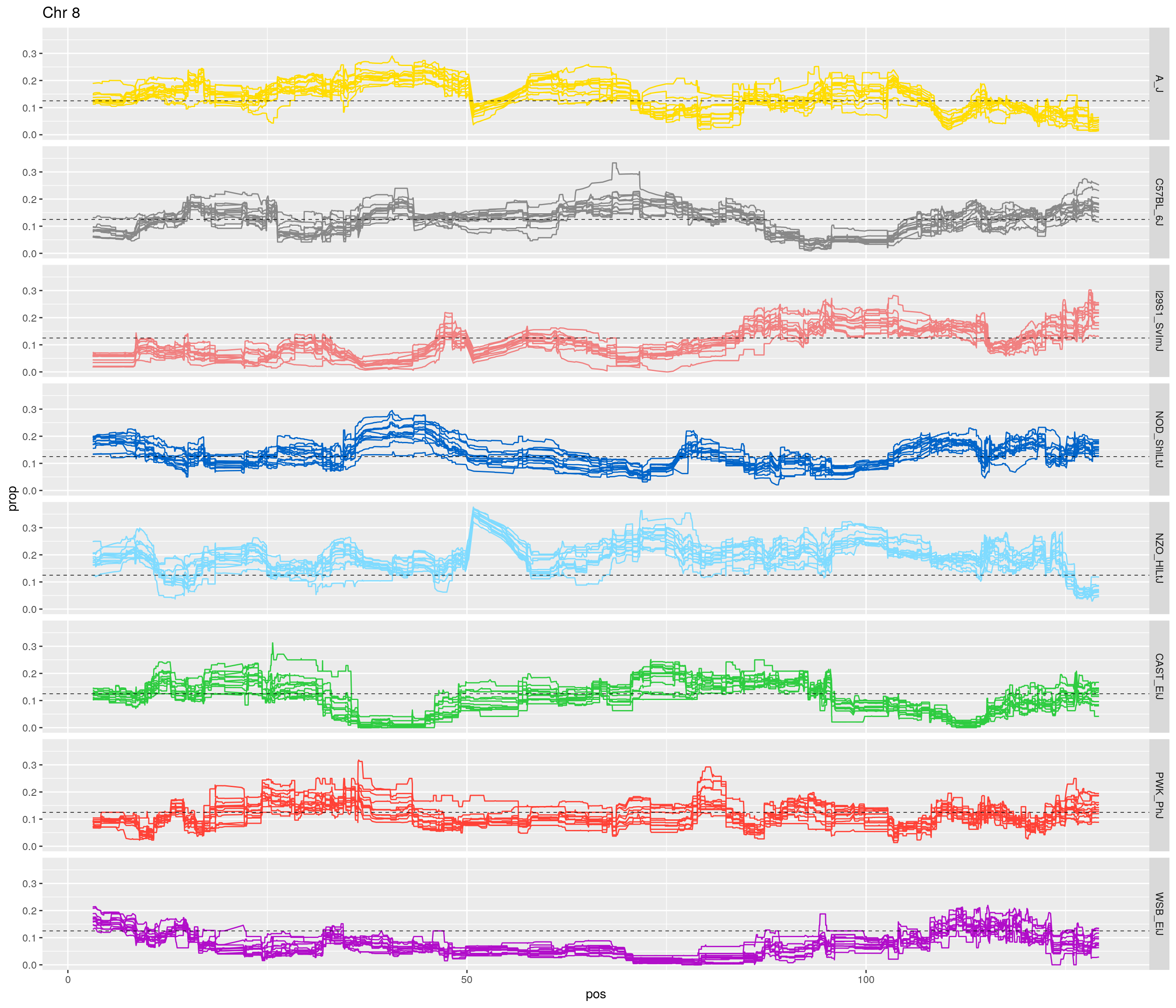
[1] "9"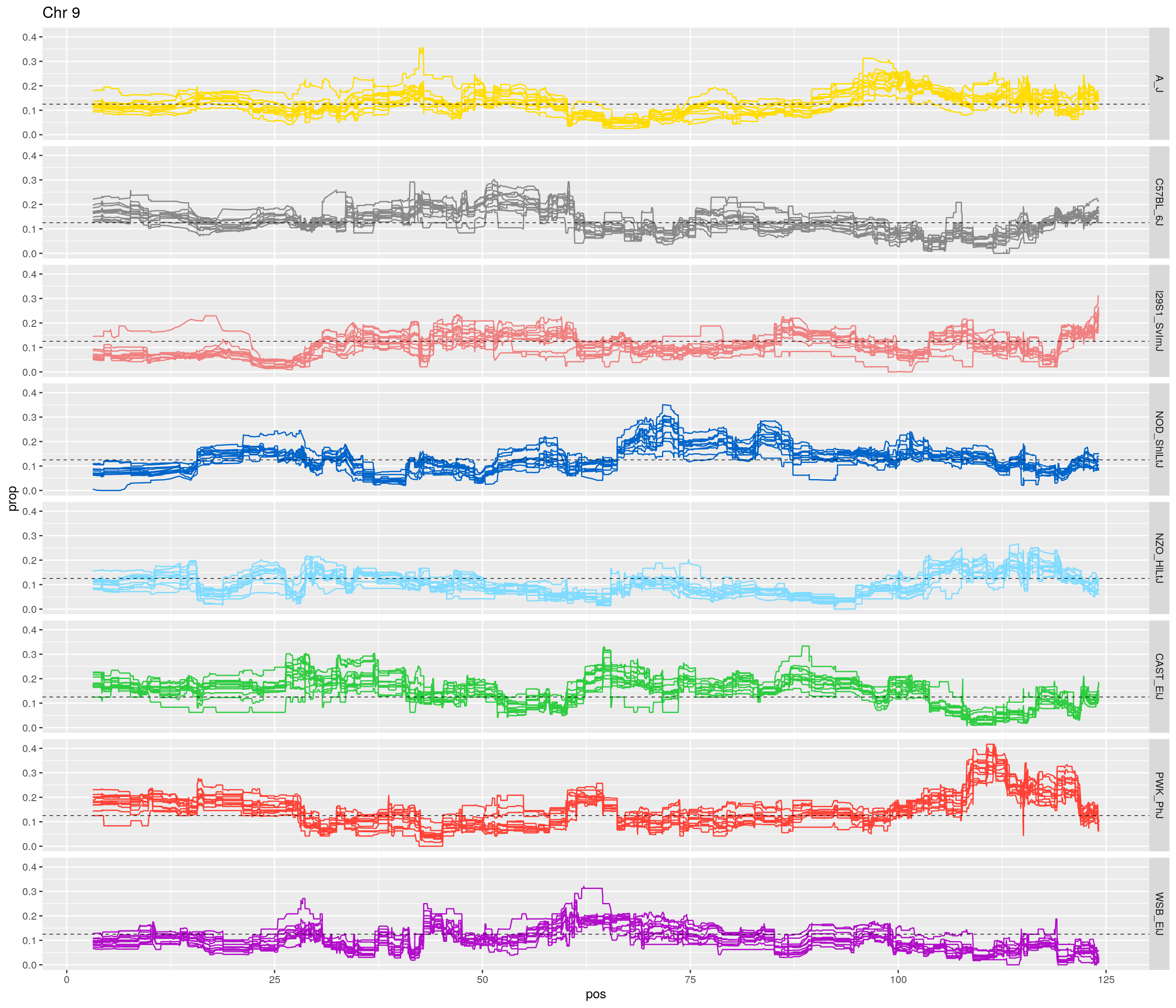
[1] "10"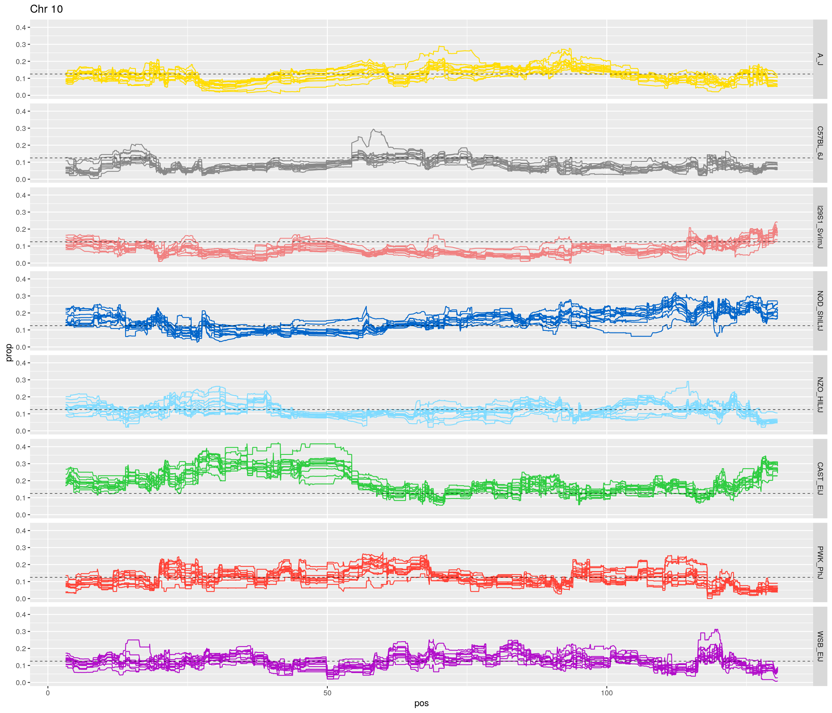
[1] "11"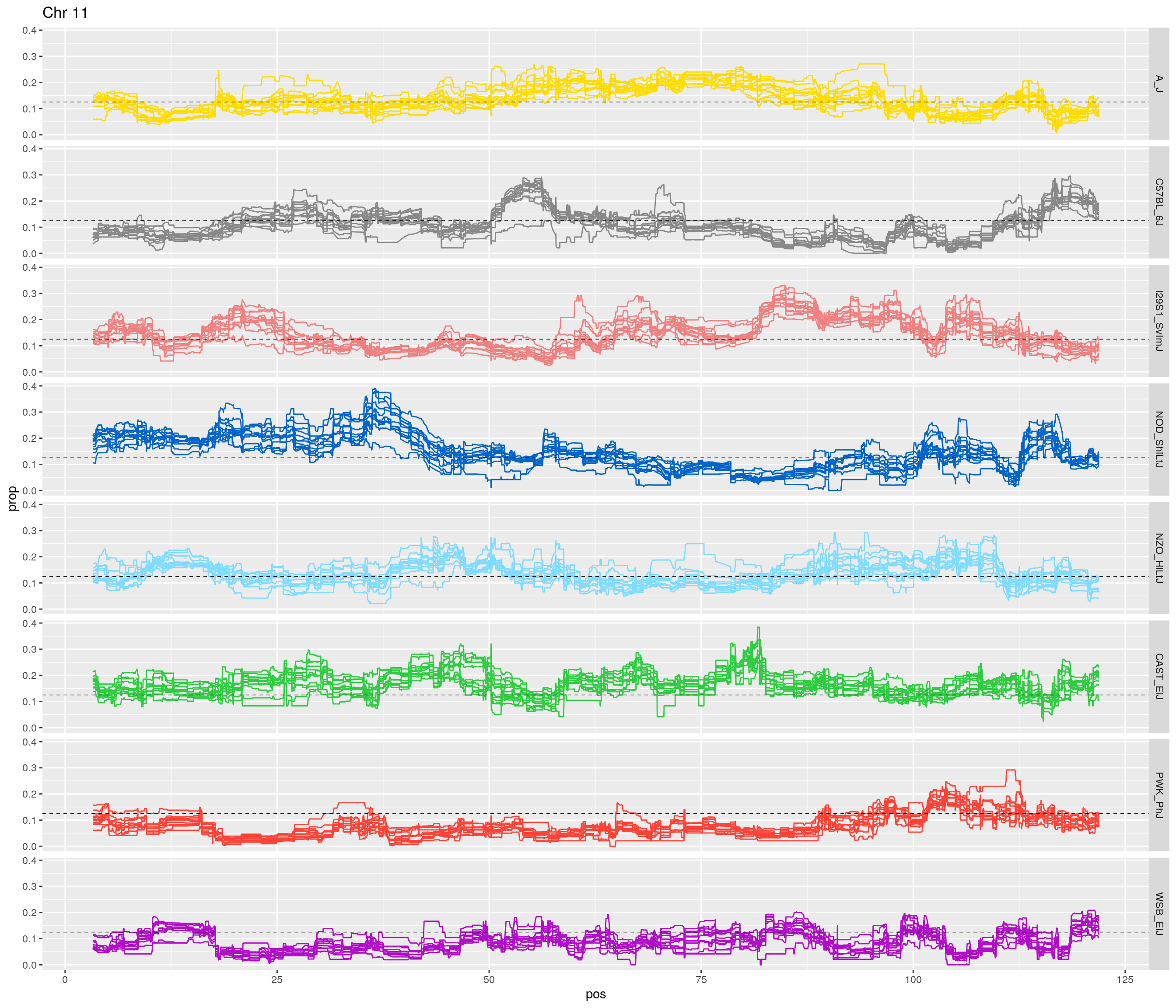
[1] "12"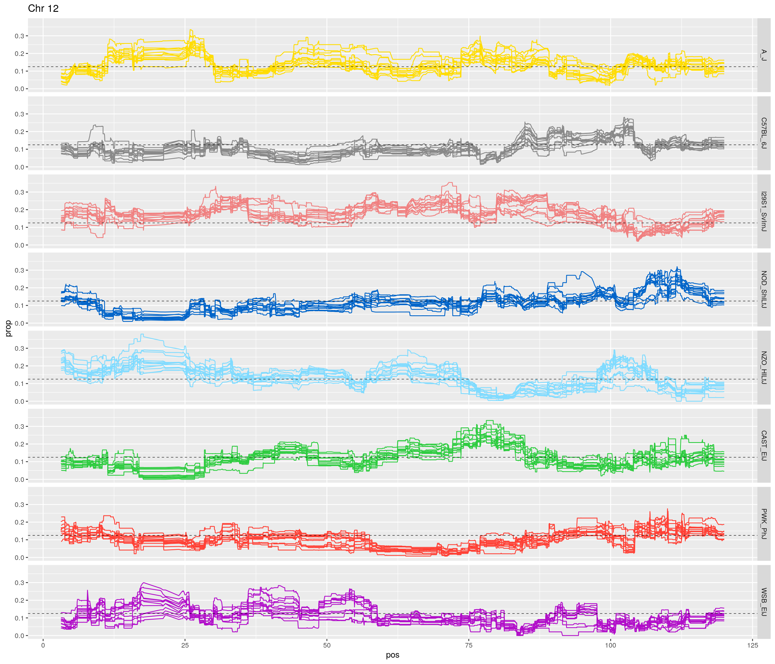
[1] "13"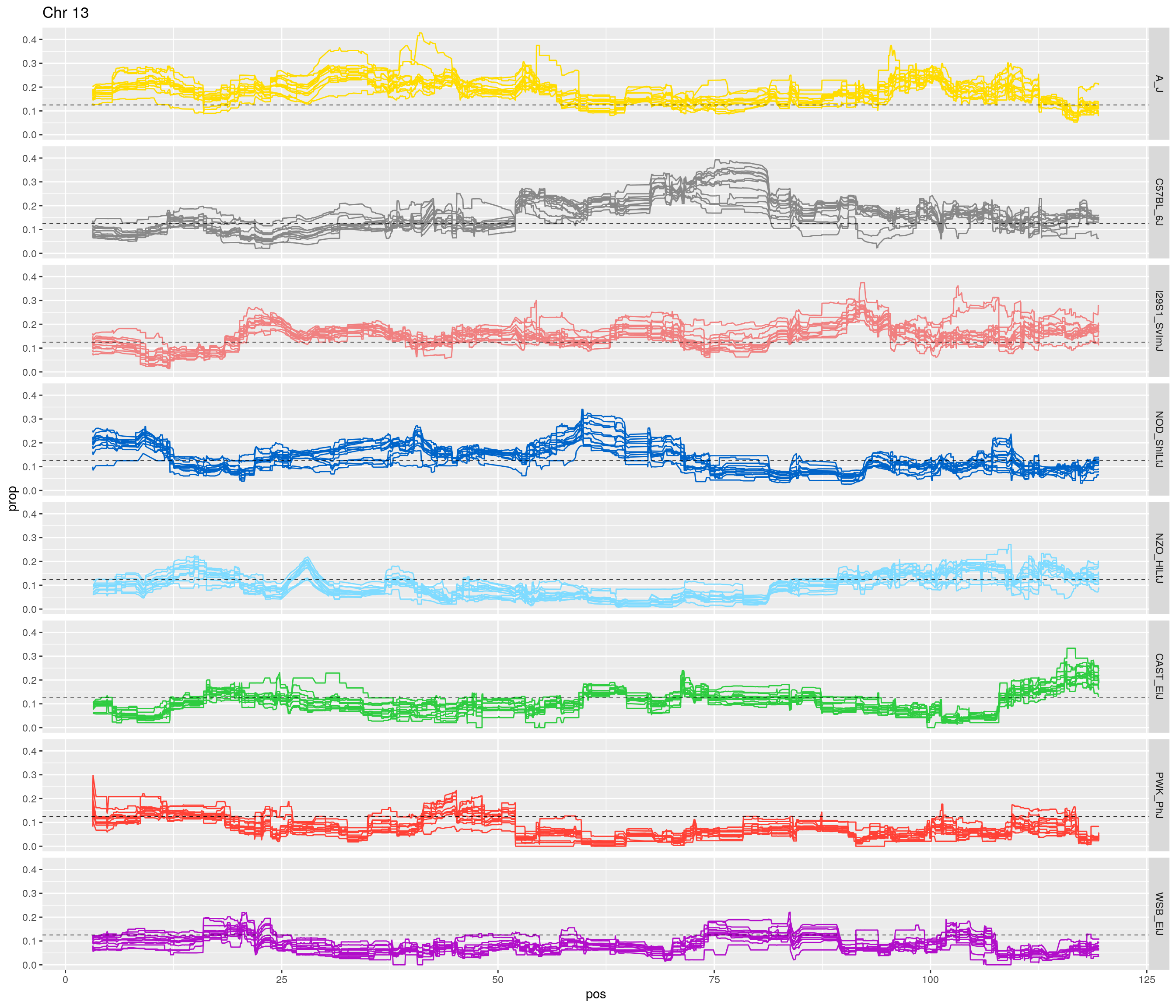
[1] "14"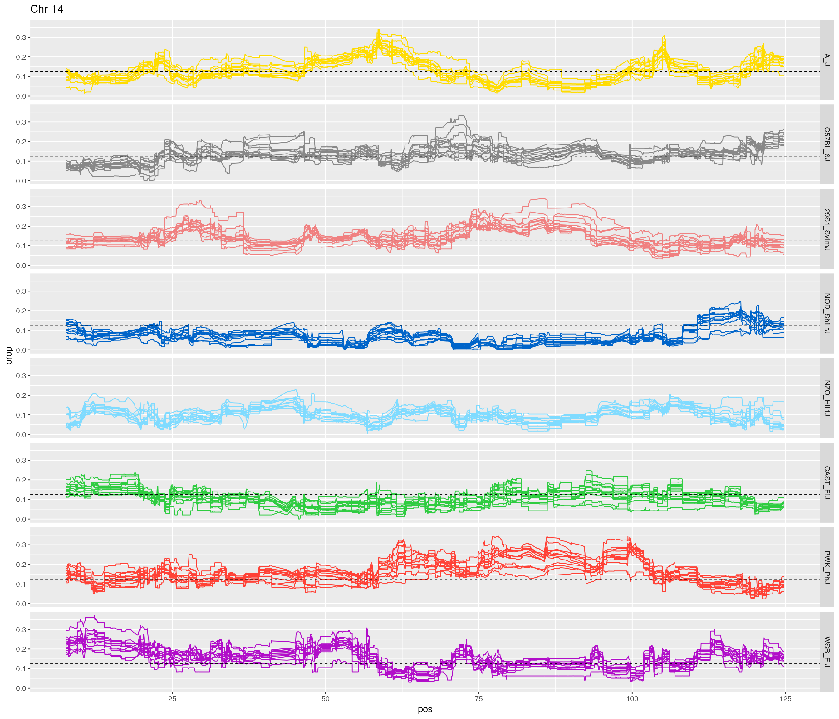
[1] "15"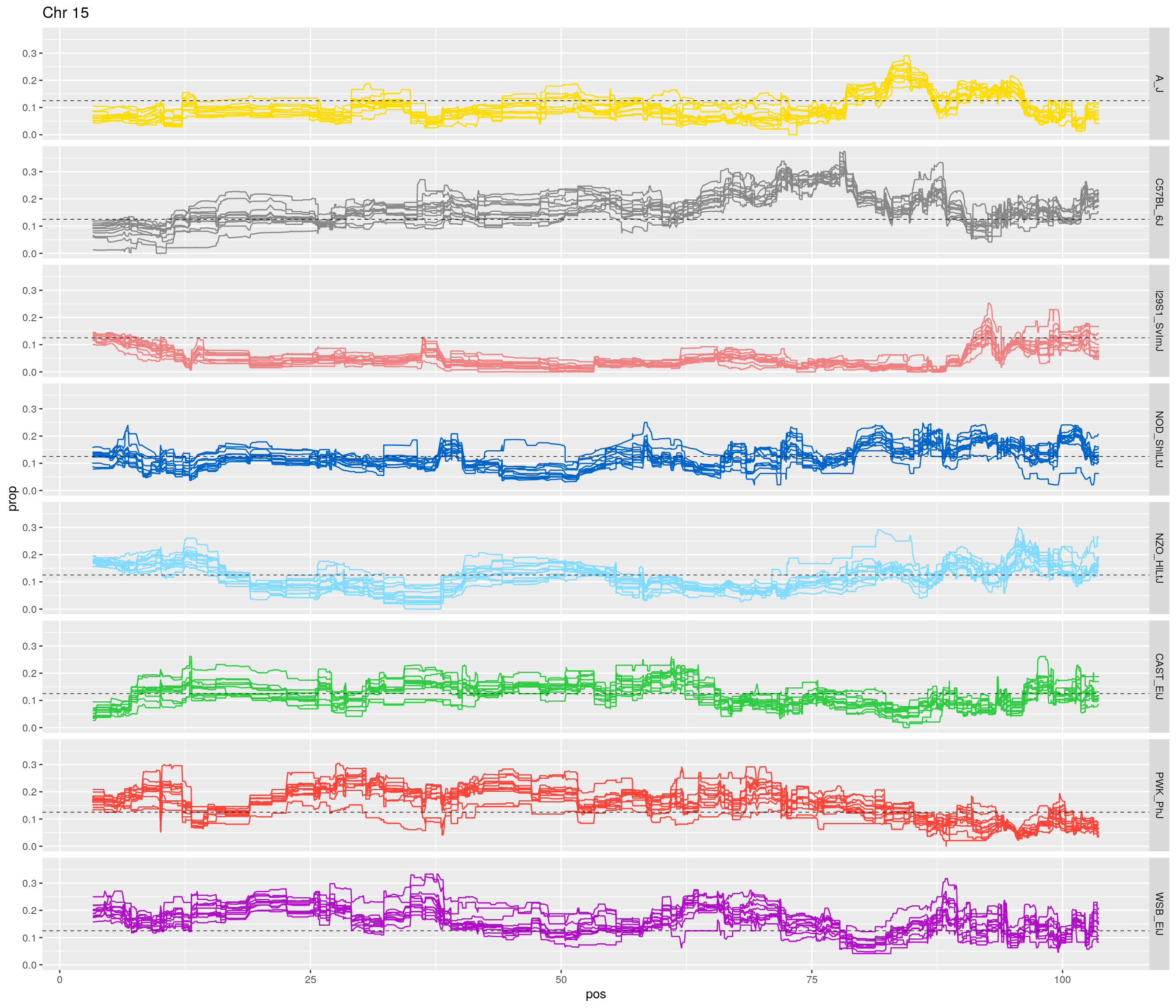
[1] "16"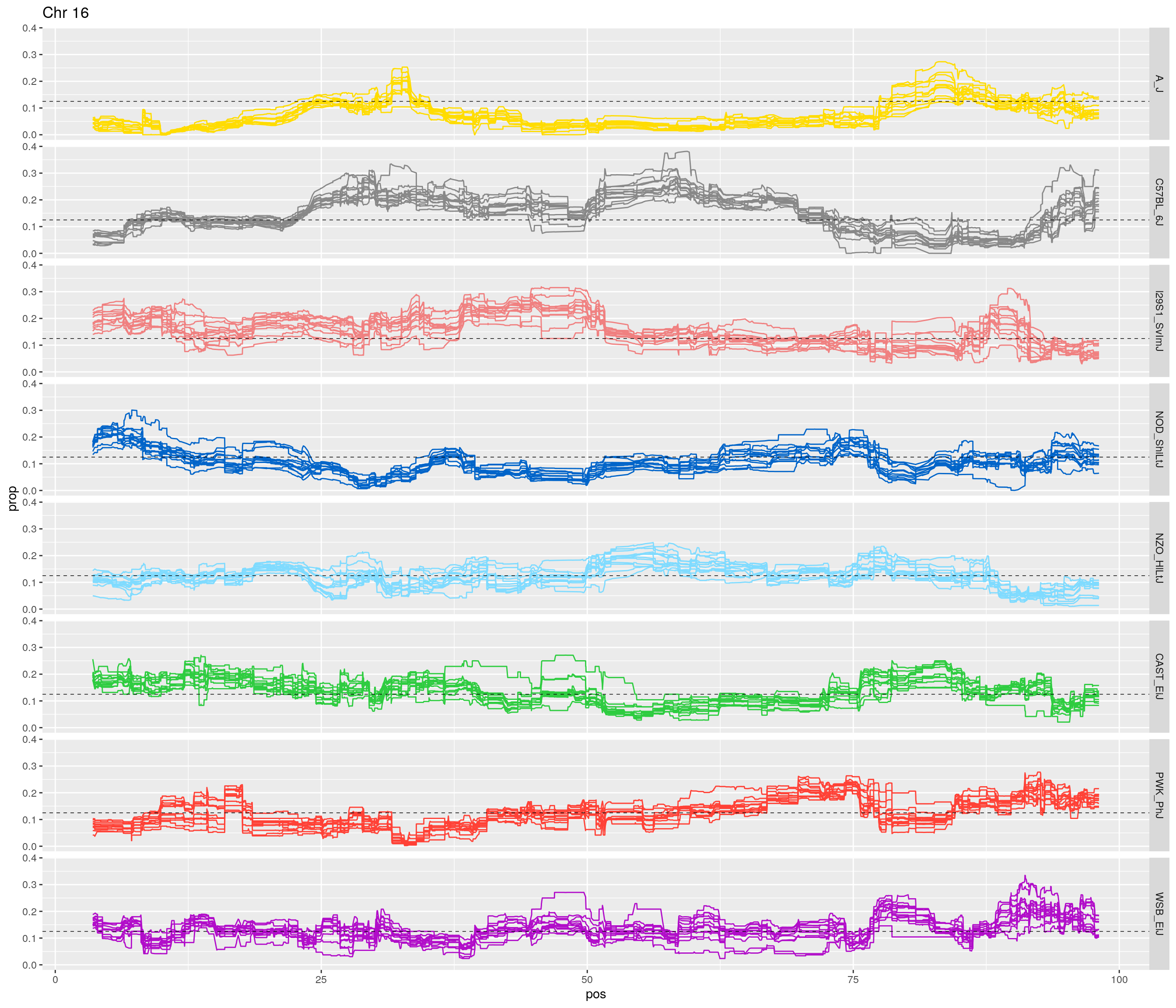
[1] "17"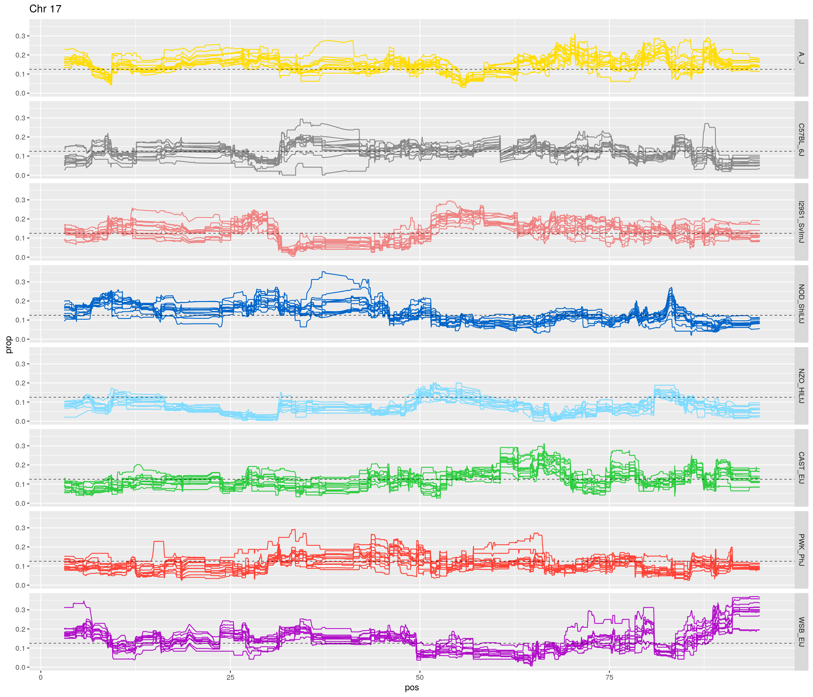
[1] "18"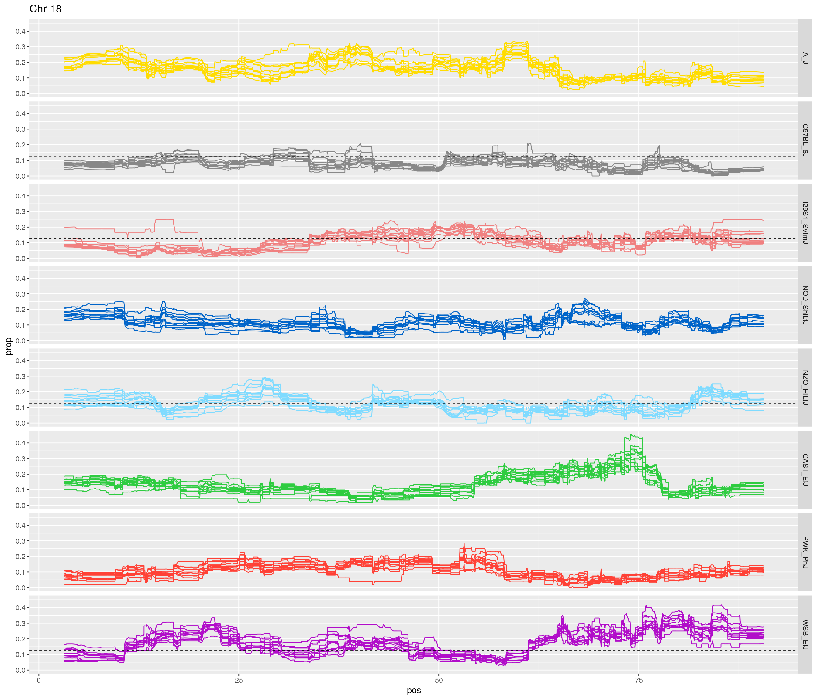
[1] "19"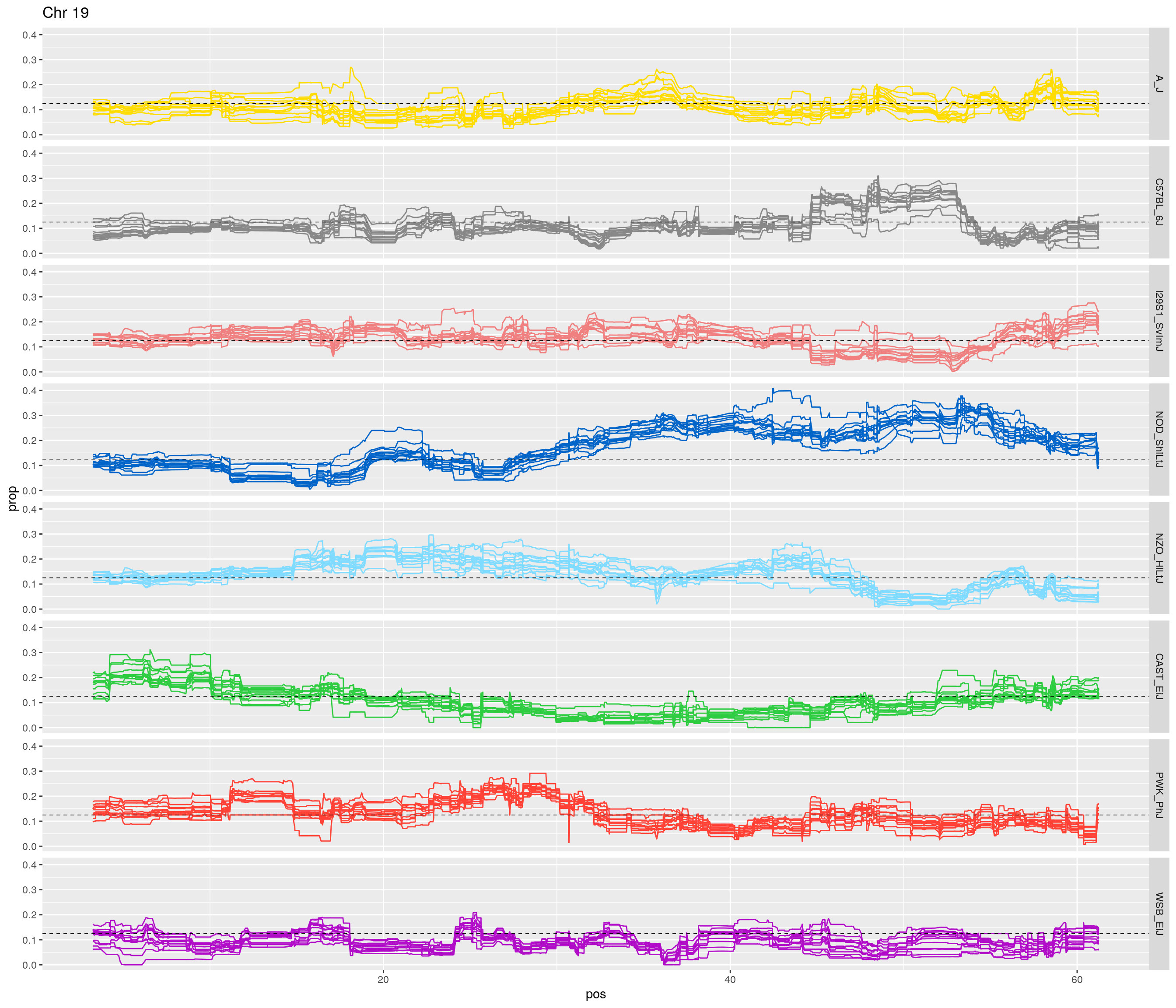
[1] "X"
#plt#Average haplotype block size
load("data/Jackson_Lab_12_batches/recom_block_size.RData")
#Create an appropriately sized vector of names
nameVector <- unlist(mapply(function(x,y){ rep(y, length(x)) }, pos_ind_gen, names(pos_ind_gen)))
#Create the result
recom_block <- cbind.data.frame(unlist(pos_ind_gen), nameVector)
colnames(recom_block) <- c("sizeblock",
                           "ngen")
#remove 0
recom_block <- recom_block[recom_block$sizeblock != 0,]
recom_block$ngen <- factor(recom_block$ngen, levels = as.character(c(21:36)))
#mean
means <- aggregate(sizeblock~ngen, data= recom_block,mean)
means$sizeblock <- round(means$sizeblock, 2)

pdf(file = "data/Jackson_Lab_12_batches/boxplot_mean_recomb_block_size.pdf", height = 8, width = 10)
p1 <- ggplot(recom_block, aes(x=ngen, y=sizeblock, group = ngen, fill = ngen)) +
  geom_boxplot(show.legend = F , outlier.size = 0.5, notchwidth = 3) +
  scale_x_discrete(drop=FALSE, breaks = c(21:23,NA,25,rep(NA,3),29:36)) +
  scale_fill_discrete_qualitative(palette = "warm")+
  geom_text(data = means, alpha = 0.85, aes(label = sizeblock, y = sizeblock + 0.15 )) +
  ylab("Recombination Block Size (Mb)") +
  xlab("Generation") +
  labs(fill = "") +
  #ylim(c(0, 60)) +
  scale_y_continuous(breaks=c(0,5,10, 20, 40, 60), limits=c(0, 60)) +
  theme(panel.grid.major = element_blank(),
        panel.grid.minor = element_blank(),
        panel.background = element_blank(),
        axis.line = element_line(colour = "black"),
        text = element_text(size=16),
        axis.title=element_text(size=16)) +
  guides(shape = guide_legend(override.aes = list(size = 12)))
p1
dev.off()
png
2 p1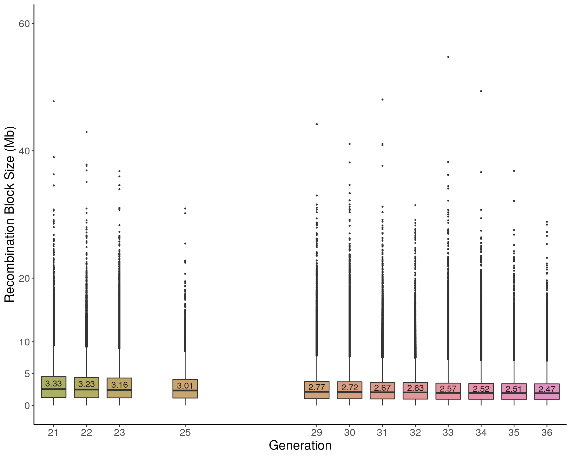
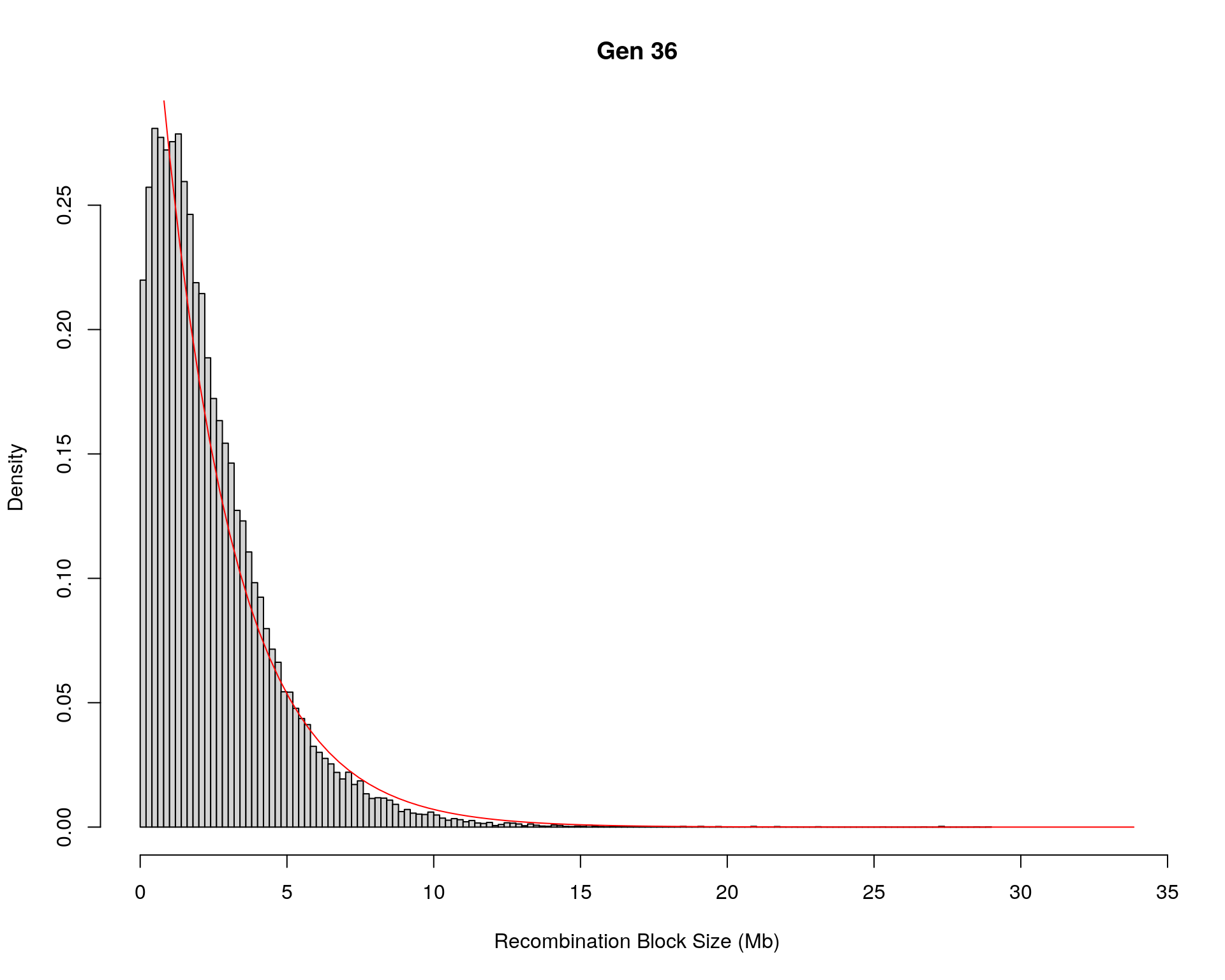
#block size distribution
for(g in unique(gm_after_qc$covar$ngen)){
  #plot for recom block size
  #png(paste0("data/Jackson_Lab_12_batches/DO_recom_block_size_G", g, ".png"))
  x <- pos_ind_gen[[g]][pos_ind_gen[[g]] != 0]
  # estimate the parameters
  fit1 <- fitdistr(x, "exponential")

  # goodness of fit test
  ks.test(x, "pexp", fit1$estimate) # p-value > 0.05 -> distribution not refused

  # plot a graph
  hist(x,
       freq = FALSE,
       breaks = 200,
       xlim = c(0, 5+quantile(x, 1)),
       #ylim = c(0,0.3),
       xlab = "Recombination Block Size (Mb)",
       main = paste0("Gen ", g))
  curve(dexp(x, rate = fit1$estimate),
        from = 0,
        to = 5+quantile(x, 1),
        col = "red",
        add = TRUE)
  #dev.off()
}
Warning in ks.test(x, "pexp", fit1$estimate): ties should not be present for the
Kolmogorov-Smirnov test
Warning in ks.test(x, "pexp", fit1$estimate): ties should not be present for the
Kolmogorov-Smirnov test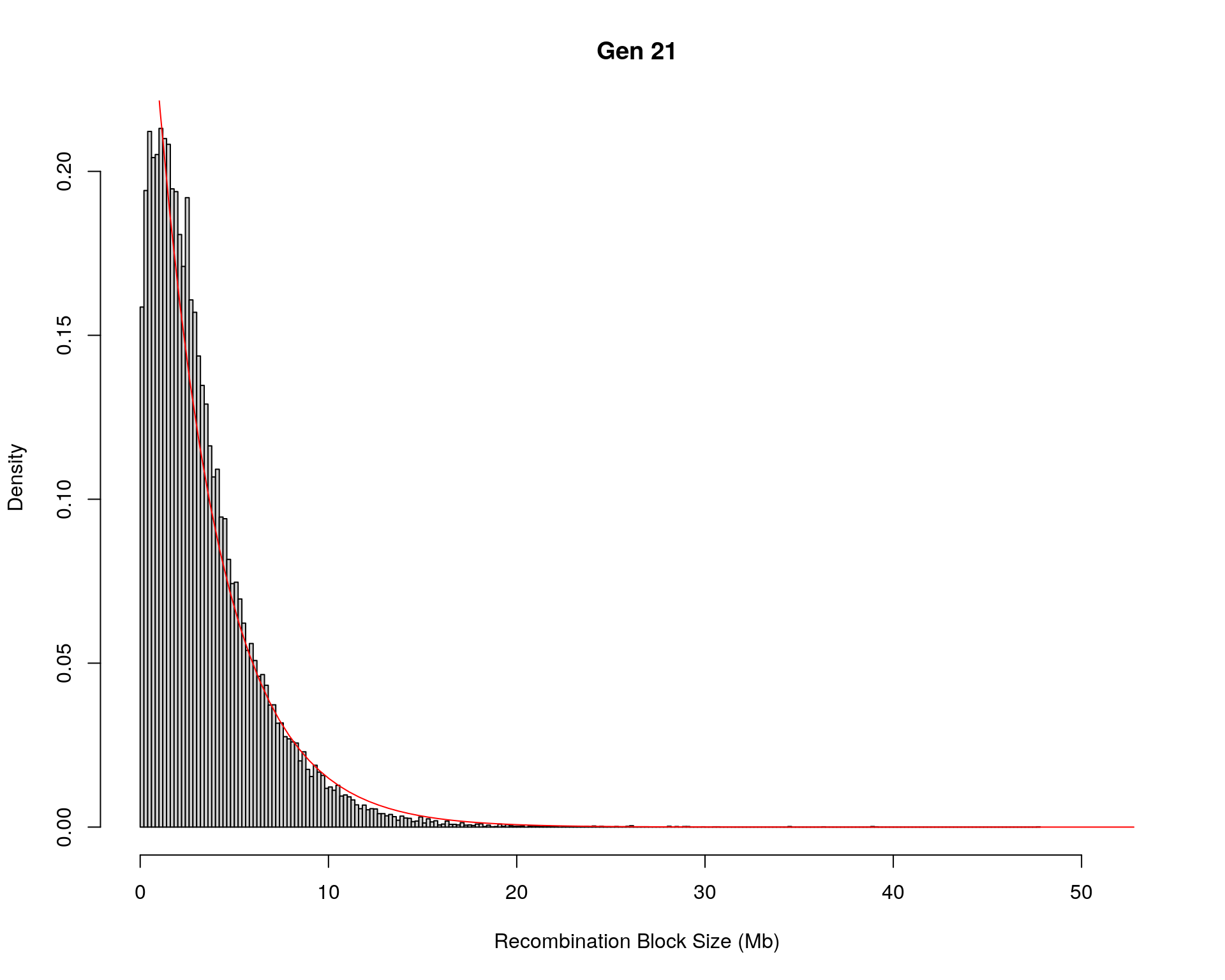
Warning in ks.test(x, "pexp", fit1$estimate): ties should not be present for the
Kolmogorov-Smirnov test
Warning in ks.test(x, "pexp", fit1$estimate): ties should not be present for the
Kolmogorov-Smirnov test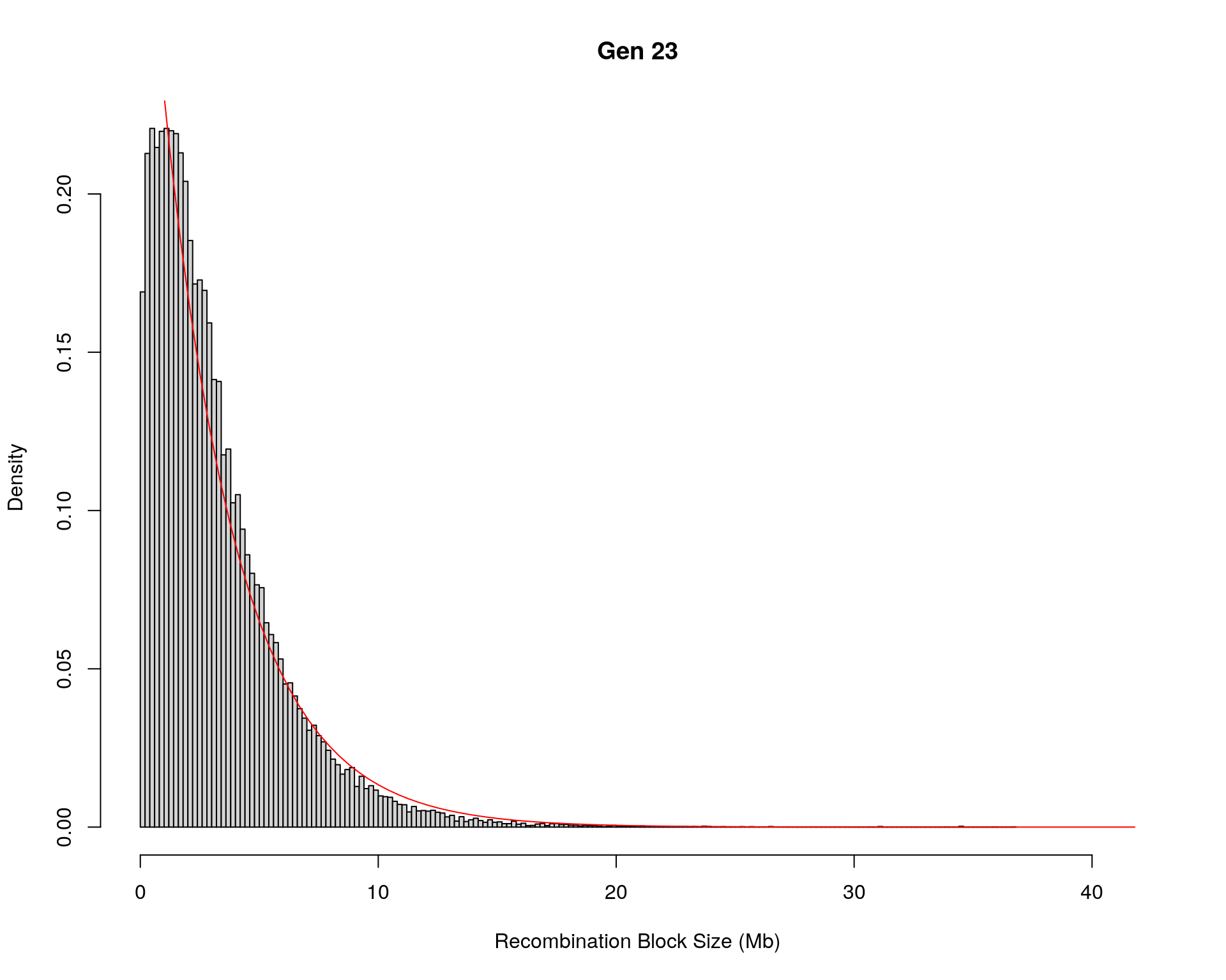
Warning in ks.test(x, "pexp", fit1$estimate): ties should not be present for the
Kolmogorov-Smirnov test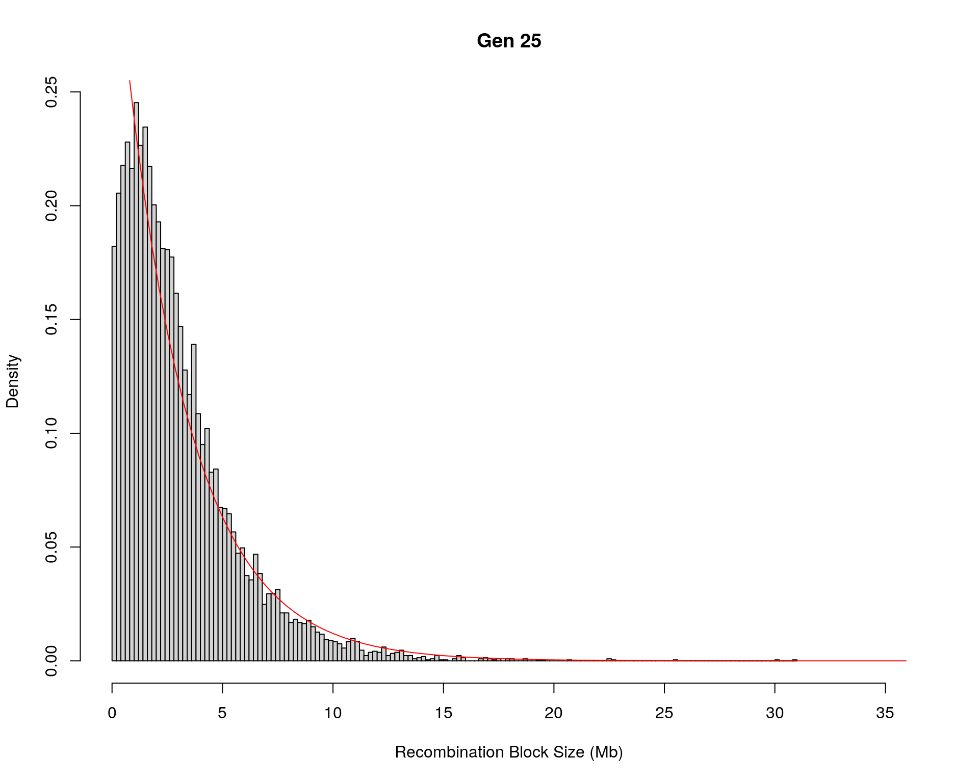
Warning in ks.test(x, "pexp", fit1$estimate): ties should not be present for the
Kolmogorov-Smirnov test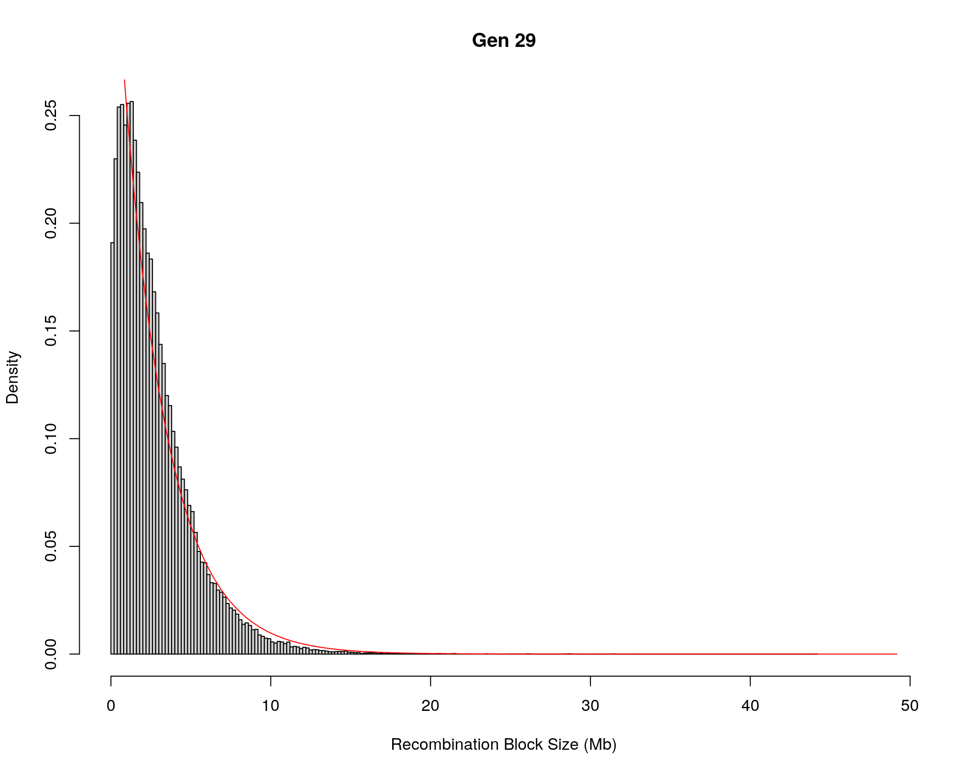
Warning in ks.test(x, "pexp", fit1$estimate): ties should not be present for the
Kolmogorov-Smirnov test
Warning in ks.test(x, "pexp", fit1$estimate): ties should not be present for the
Kolmogorov-Smirnov test
Warning in ks.test(x, "pexp", fit1$estimate): ties should not be present for the
Kolmogorov-Smirnov test
Warning in ks.test(x, "pexp", fit1$estimate): ties should not be present for the
Kolmogorov-Smirnov test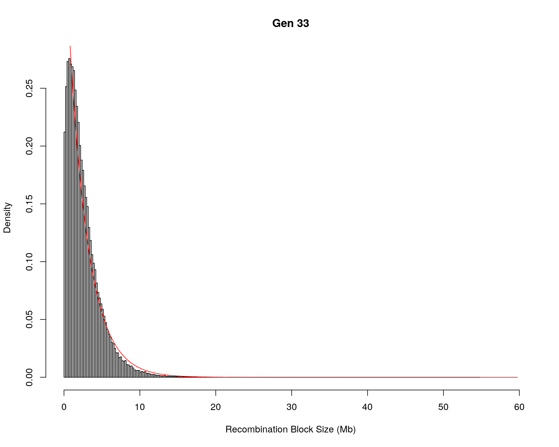
Warning in ks.test(x, "pexp", fit1$estimate): ties should not be present for the
Kolmogorov-Smirnov test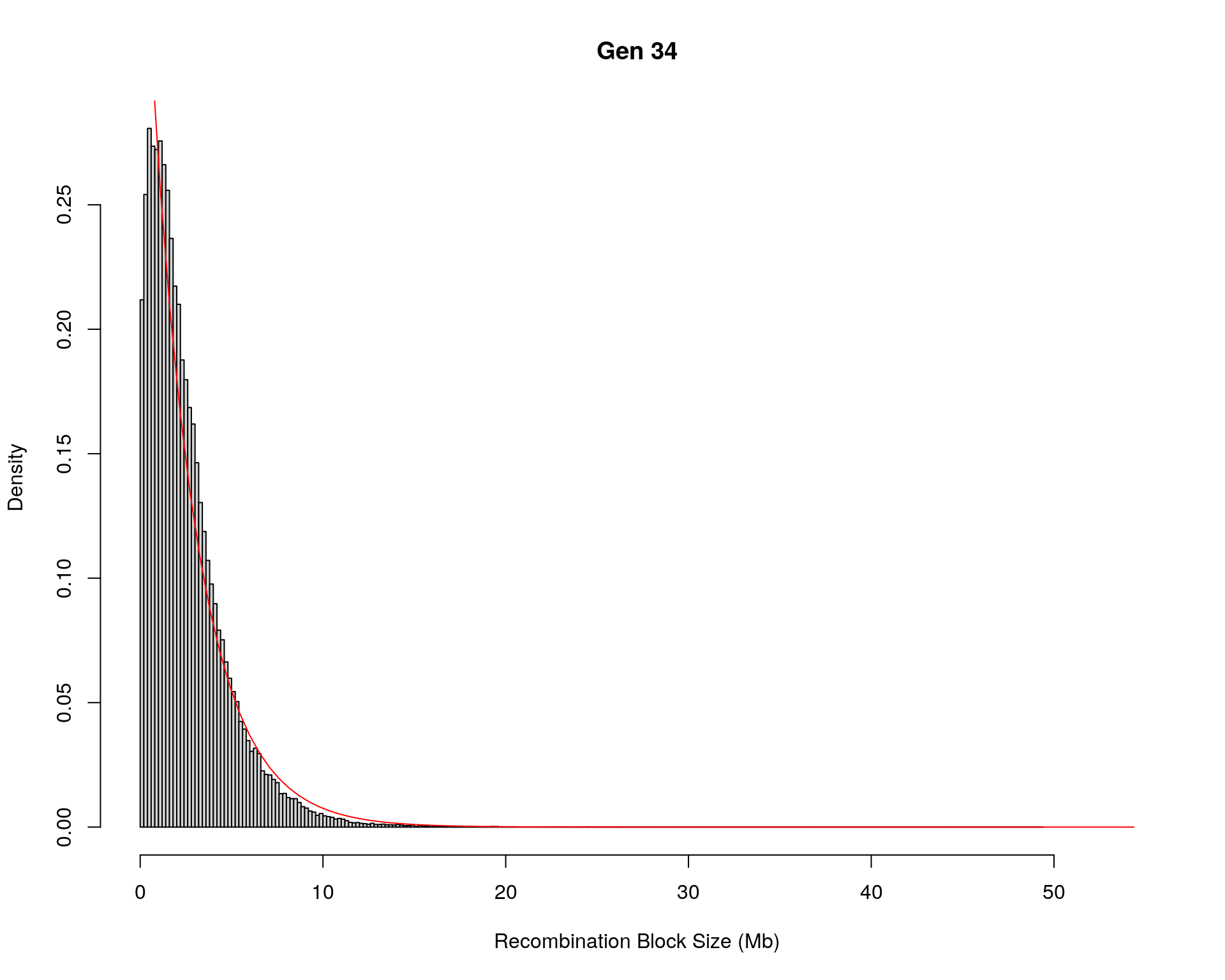
Warning in ks.test(x, "pexp", fit1$estimate): ties should not be present for the
Kolmogorov-Smirnov test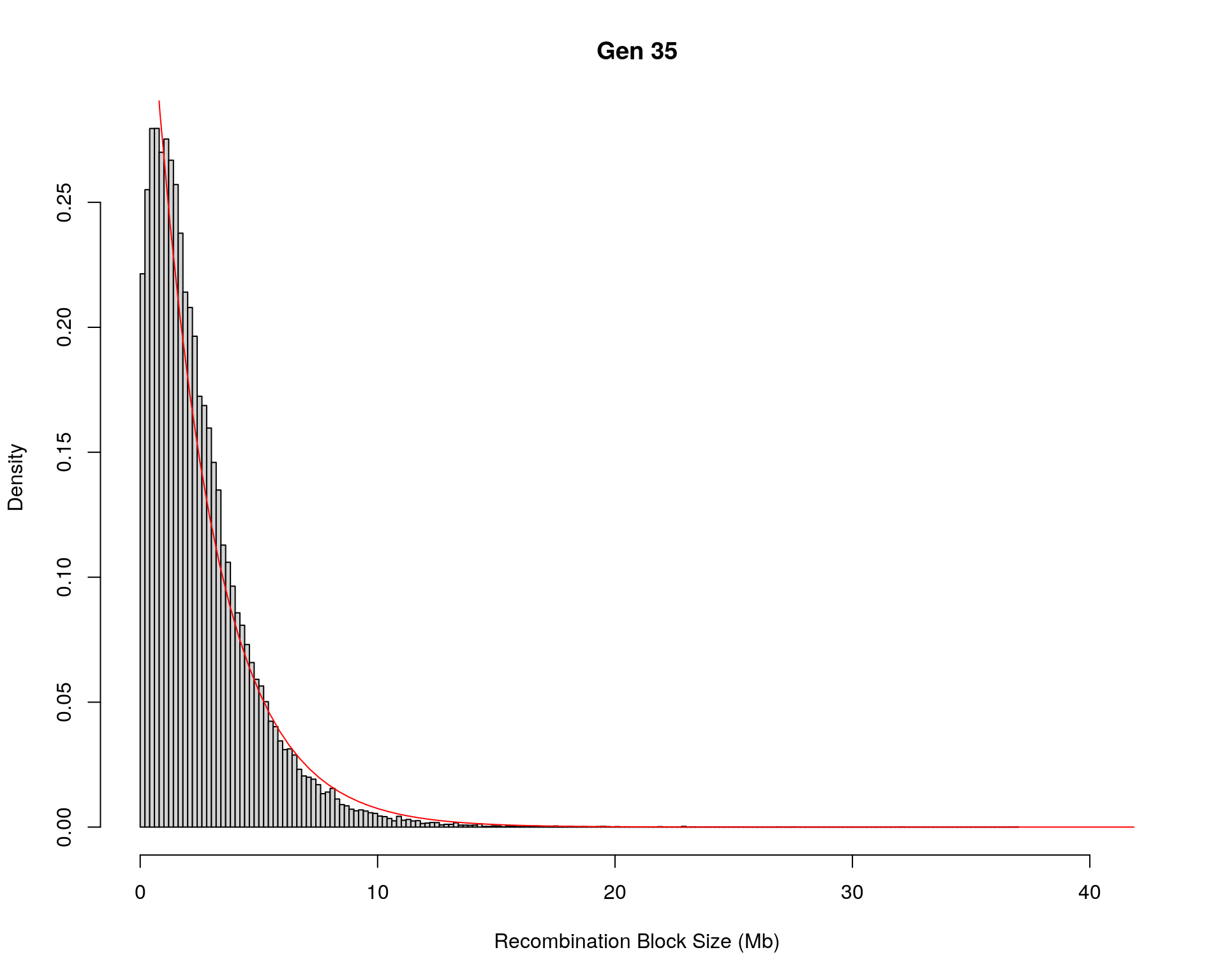
#Average heterozygosity value
load("data/Jackson_Lab_12_batches/dat_het_ind_pr.RData")
dat_het_ind_pr$ngen <- factor(dat_het_ind_pr$ngen, levels = as.character(c(21:36)))

pdf(paste("data/Jackson_Lab_12_batches/DO_Heterozygosity_value_violin_genoprops.pdf"), width = 10, height =8)
p2 <- ggplot(dat_het_ind_pr, aes(x=ngen, y=het, group=ngen, fill=ngen)) +
  geom_violin(show.legend = FALSE) +
  geom_boxplot(show.legend = FALSE, width=0.35, color="black", alpha=0.6) +
  scale_x_discrete(drop=FALSE, breaks = c(21:23,NA,25,rep(NA,3),29:36)) +
  scale_fill_discrete_qualitative(palette = "warm")+
  ylab("Heterozygosity from genotype props") +
  xlab("Generation") +
  ylim(c(0.65, 1)) +
  geom_hline(yintercept=0.875, linetype="dashed", color = "red") +
  #scale_y_continuous(breaks=c(0.55, 0.65, 0.75, 0.85, 0.95, 1), limits=c(0.55, 1)) +
  theme(panel.grid.major = element_blank(),
        panel.grid.minor = element_blank(),
        panel.background = element_blank(),
        axis.line = element_line(colour = "black"),
        text = element_text(size=16),
        axis.title=element_text(size=16),
        legend.title=element_blank())
p2
dev.off()
png
2 p2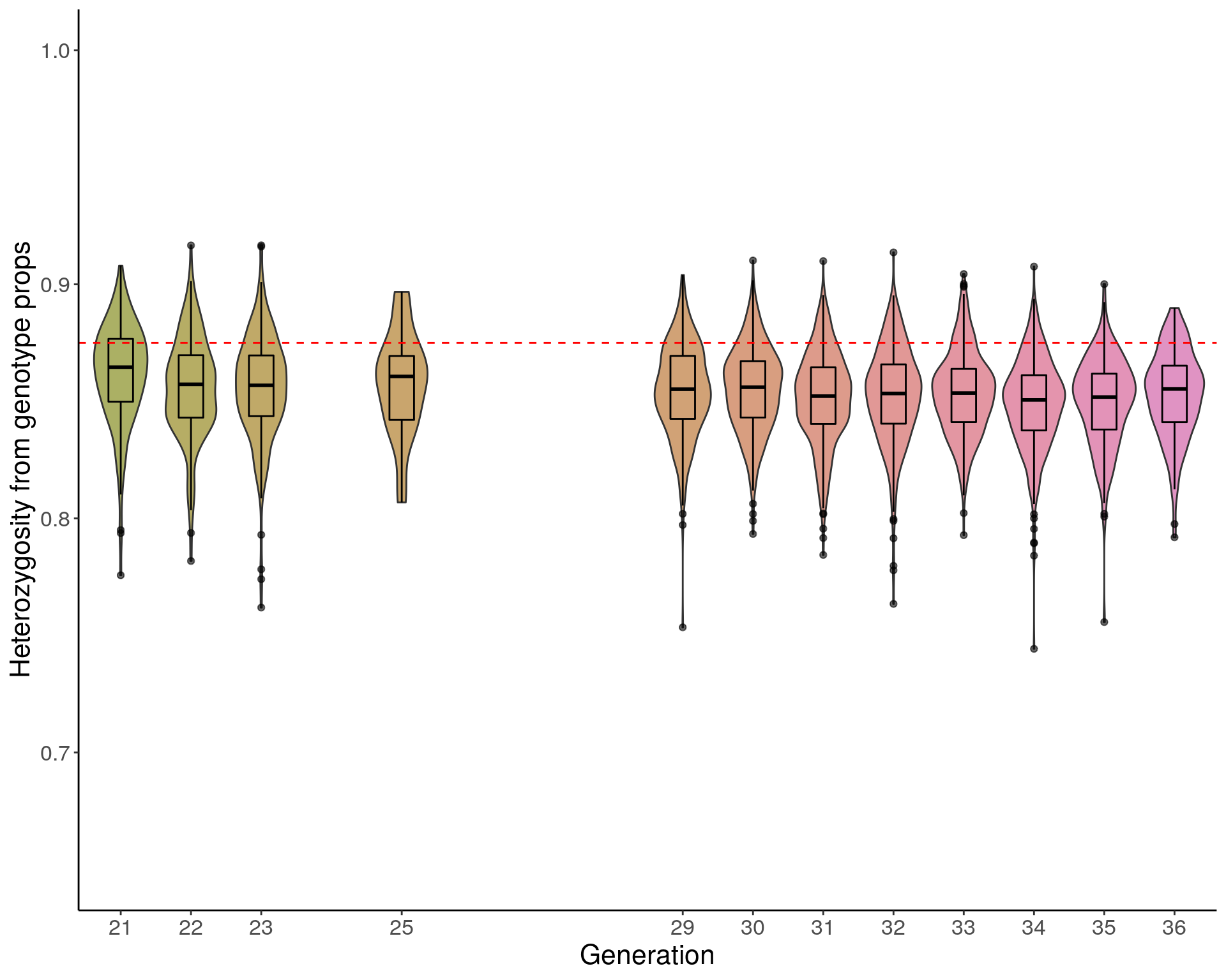
#marker UNC13316610 allele frequency
T_freq <- unique(gm_after_qc$covar$ngen) %>%
  map(~(read.table(paste0("data/GCTA/12_batches_QC_id_gen", .x,".frq"), header = TRUE) %>%
          filter(SNP == "UNC13316610") %>%
          mutate(GEN = .x, .before = 1))
        ) %>%
  set_names(., nm = unique(gm_after_qc$covar$ngen)) %>%
  bind_rows() %>%
  mutate(allele = "T",
         MAF_allele = case_when(
           A1 == "T" ~ MAF,
           A1 != "T" ~ 1-MAF
         ))
C_freq <- T_freq %>%
  mutate(allele = "C",
         MAF_allele = 1-MAF_allele
         )
#bind
UNC13316610.freq <- bind_rows(T_freq, C_freq)
# Stacked
p <- ggplot(UNC13316610.freq, aes(fill=allele, y=MAF_allele, x=GEN)) +
  geom_bar(position="stack", stat="identity") +
  scale_fill_manual(values=c("#3399CC", "#FFCC33")) +
  xlab("Generation") +
  ylab("UNC13316610 allele frequency")
print(p)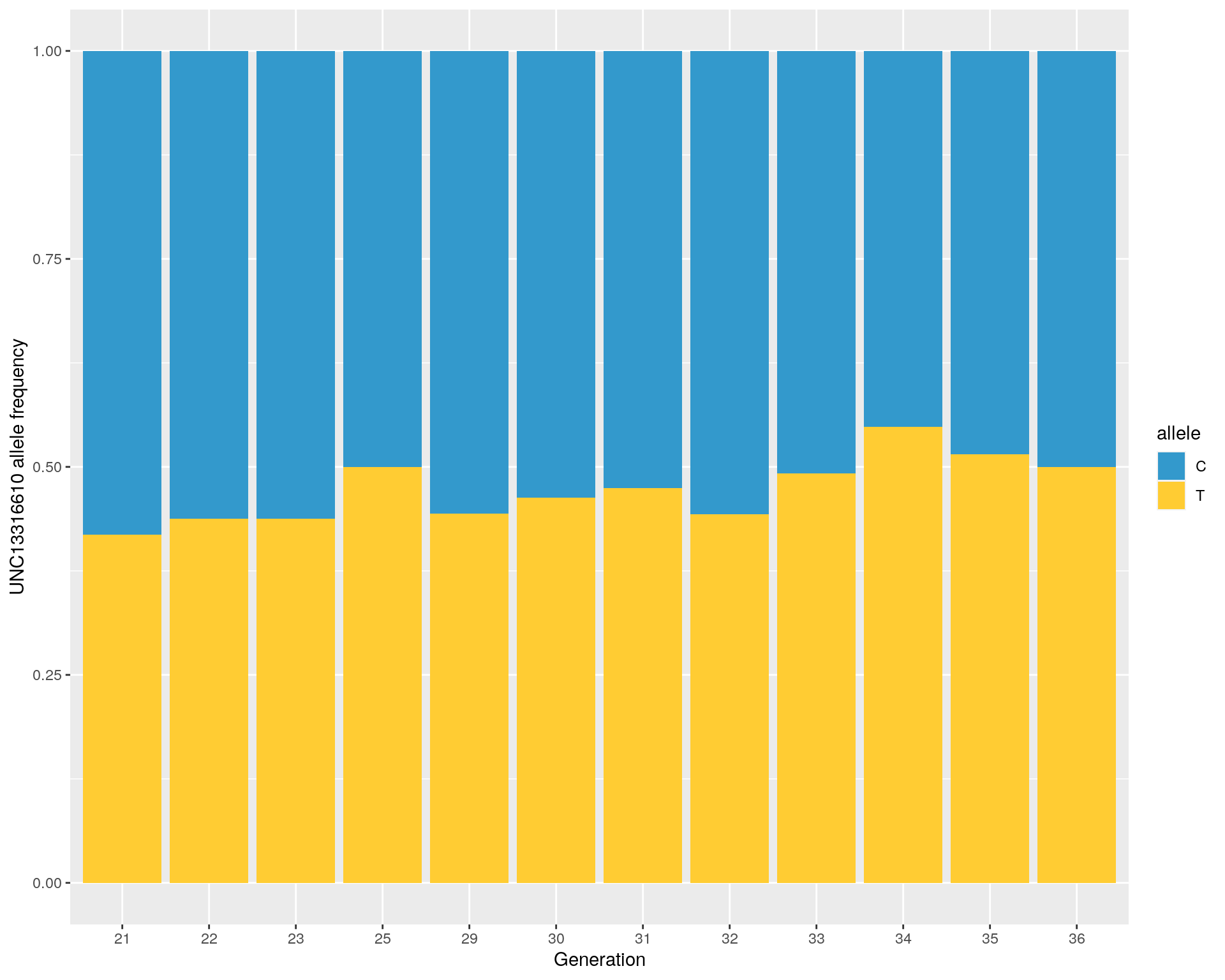
| Version | Author | Date |
|---|---|---|
| d35c8a5 | xhyuo | 2021-06-16 |
#pull marker UNC13316610
gm.UNC13316610 <- pull_markers(gm_after_qc, "UNC13316610")
#genotype freq
gfreq <- calc_raw_geno_freq(gm.UNC13316610)
gfreq_tab <- gfreq %>%
  as.data.frame() %>%
  mutate(id = rownames(gfreq)) %>%
  left_join(gm_after_qc$covar) %>%
  group_by(ngen)

#gfreq_tab
tab <- gfreq_tab %>%
  group_map(~(apply(.x[,1:3],2,function(x)(sum(x,na.rm = T))))) %>%
  bind_rows() %>%
  mutate(Genertation = group_keys(gfreq_tab)$ngen, .before = 1) %>%
  left_join(C_freq[,c("GEN", "MAF_allele")], by = c("Genertation" = "GEN")) %>%
  left_join(T_freq[,c("GEN", "MAF_allele")], by = c("Genertation" = "GEN")) %>%
  rename(C_freq = MAF_allele.x) %>%
  rename(T_freq = MAF_allele.y) %>%
  mutate(C_freq2 = (2*AA + AB)/(2*(AA+AB+BB))) %>%
  rowwise() %>%
  mutate(chisq = HWChisq(c(AA, AB, BB))$chisq,
         df    = HWChisq(c(AA, AB, BB))$df,
         p     = HWChisq(c(AA, AB, BB))$p) %>%
  dplyr::select(Genertation = Genertation,
                CC = AA,
                CT = AB,
                TT = BB,
                C_freq,
                T_freq,
                chisq,
                p)
Chi-square test with continuity correction for Hardy-Weinberg equilibrium (autosomal)
Chi2 = 3.64016 DF = 1 p-value = 0.05640151 D = -6.027027 f = 0.1672918
Chi-square test with continuity correction for Hardy-Weinberg equilibrium (autosomal)
Chi2 = 0.0139537 DF = 1 p-value = 0.905968 D = -0.03870968 f = 0.001017639
Chi-square test with continuity correction for Hardy-Weinberg equilibrium (autosomal)
Chi2 = 0.5915421 DF = 1 p-value = 0.4418234 D = -3.003886 f = 0.06323453
Chi-square test with continuity correction for Hardy-Weinberg equilibrium (autosomal)
Chi2 = 0.1041667 DF = 1 p-value = 0.7468856 D = 0 f = 0
Chi-square test with continuity correction for Hardy-Weinberg equilibrium (autosomal)
Chi2 = 2.206823 DF = 1 p-value = 0.1374014 D = 7.037121 f = -0.08638439
Chi-square test with continuity correction for Hardy-Weinberg equilibrium (autosomal)
Chi2 = 0.07948221 DF = 1 p-value = 0.7780003 D = 1.835812 f = -0.01689436
Chi-square test with continuity correction for Hardy-Weinberg equilibrium (autosomal)
Chi2 = 0.01635285 DF = 1 p-value = 0.8982453 D = 1.014388 f = -0.009755085
Chi-square test with continuity correction for Hardy-Weinberg equilibrium (autosomal)
Chi2 = 0.582596 DF = 1 p-value = 0.4452966 D = -3.727918 f = 0.04765457
Chi-square test with continuity correction for Hardy-Weinberg equilibrium (autosomal)
Chi2 = 0.250779 DF = 1 p-value = 0.6165271 D = 3.027222 f = -0.02691515
Chi-square test with continuity correction for Hardy-Weinberg equilibrium (autosomal)
Chi2 = 2.441985 DF = 1 p-value = 0.1181267 D = 8.184275 f = -0.08118054
Chi-square test with continuity correction for Hardy-Weinberg equilibrium (autosomal)
Chi2 = 1.695457 DF = 1 p-value = 0.1928832 D = 4.53811 f = -0.1107886
Chi-square test with continuity correction for Hardy-Weinberg equilibrium (autosomal)
Chi2 = 0.1576923 DF = 1 p-value = 0.6912901 D = -1.5 f = 0.04615385
Chi-square test with continuity correction for Hardy-Weinberg equilibrium (autosomal)
Chi2 = 3.64016 DF = 1 p-value = 0.05640151 D = -6.027027 f = 0.1672918
Chi-square test with continuity correction for Hardy-Weinberg equilibrium (autosomal)
Chi2 = 0.0139537 DF = 1 p-value = 0.905968 D = -0.03870968 f = 0.001017639
Chi-square test with continuity correction for Hardy-Weinberg equilibrium (autosomal)
Chi2 = 0.5915421 DF = 1 p-value = 0.4418234 D = -3.003886 f = 0.06323453
Chi-square test with continuity correction for Hardy-Weinberg equilibrium (autosomal)
Chi2 = 0.1041667 DF = 1 p-value = 0.7468856 D = 0 f = 0
Chi-square test with continuity correction for Hardy-Weinberg equilibrium (autosomal)
Chi2 = 2.206823 DF = 1 p-value = 0.1374014 D = 7.037121 f = -0.08638439
Chi-square test with continuity correction for Hardy-Weinberg equilibrium (autosomal)
Chi2 = 0.07948221 DF = 1 p-value = 0.7780003 D = 1.835812 f = -0.01689436
Chi-square test with continuity correction for Hardy-Weinberg equilibrium (autosomal)
Chi2 = 0.01635285 DF = 1 p-value = 0.8982453 D = 1.014388 f = -0.009755085
Chi-square test with continuity correction for Hardy-Weinberg equilibrium (autosomal)
Chi2 = 0.582596 DF = 1 p-value = 0.4452966 D = -3.727918 f = 0.04765457
Chi-square test with continuity correction for Hardy-Weinberg equilibrium (autosomal)
Chi2 = 0.250779 DF = 1 p-value = 0.6165271 D = 3.027222 f = -0.02691515
Chi-square test with continuity correction for Hardy-Weinberg equilibrium (autosomal)
Chi2 = 2.441985 DF = 1 p-value = 0.1181267 D = 8.184275 f = -0.08118054
Chi-square test with continuity correction for Hardy-Weinberg equilibrium (autosomal)
Chi2 = 1.695457 DF = 1 p-value = 0.1928832 D = 4.53811 f = -0.1107886
Chi-square test with continuity correction for Hardy-Weinberg equilibrium (autosomal)
Chi2 = 0.1576923 DF = 1 p-value = 0.6912901 D = -1.5 f = 0.04615385 tab# A tibble: 12 x 8
# Rowwise:
Genertation CC CT TT C_freq T_freq chisq p
<chr> <dbl> <dbl> <dbl> <dbl> <dbl> <dbl> <dbl>
1 21 56 60 32 0.581 0.419 3.64 0.419
2 22 50 76 29 0.562 0.438 0.0140 0.432
3 23 64 89 40 0.562 0.438 0.592 0.438
4 25 6 12 6 0.5 0.5 0.104 0.5
5 29 95 177 58 0.556 0.444 2.21 0.444
6 30 124 221 92 0.537 0.463 0.0795 0.463
7 31 114 210 93 0.525 0.475 0.0164 0.475
8 32 102 149 66 0.557 0.443 0.583 0.443
9 33 113 231 106 0.508 0.492 0.251 0.492
10 34 75 218 114 0.452 0.548 2.44 0.452
11 35 34 91 39 0.485 0.515 1.70 0.485
12 36 34 62 34 0.5 0.5 0.158 0.5
sessionInfo()R version 4.0.3 (2020-10-10)
Platform: x86_64-pc-linux-gnu (64-bit)
Running under: Ubuntu 20.04.1 LTS
Matrix products: default
BLAS/LAPACK: /usr/lib/x86_64-linux-gnu/openblas-pthread/libopenblasp-r0.3.8.so
locale:
[1] LC_CTYPE=en_US.UTF-8 LC_NUMERIC=C
[3] LC_TIME=en_US.UTF-8 LC_COLLATE=en_US.UTF-8
[5] LC_MONETARY=en_US.UTF-8 LC_MESSAGES=C
[7] LC_PAPER=en_US.UTF-8 LC_NAME=C
[9] LC_ADDRESS=C LC_TELEPHONE=C
[11] LC_MEASUREMENT=en_US.UTF-8 LC_IDENTIFICATION=C
attached base packages:
[1] grid parallel stats graphics grDevices utils datasets
[8] methods base
other attached packages:
[1] DOQTL_1.0.0 HardyWeinberg_1.7.2 Rsolnp_1.16
[4] mice_3.12.0 colorspace_2.0-0 MASS_7.3-53
[7] vcd_1.4-8 lme4_1.1-26 Matrix_1.2-18
[10] regress_1.3-21 gap_1.2.2 abind_1.4-5
[13] doParallel_1.0.16 iterators_1.0.13 foreach_1.5.1
[16] data.table_1.13.6 forcats_0.5.0 stringr_1.4.0
[19] dplyr_1.0.2 purrr_0.3.4 readr_1.4.0
[22] tidyr_1.1.2 tibble_3.0.4 ggplot2_3.3.2
[25] tidyverse_1.3.0 table1_1.2.1 qtl2_0.24
[28] workflowr_1.6.2
loaded via a namespace (and not attached):
[1] readxl_1.3.1 MUGAExampleData_1.10.0 backports_1.2.0
[4] BiocFileCache_1.14.0 splines_4.0.3 BiocParallel_1.22.0
[7] GenomeInfoDb_1.26.2 digest_0.6.27 htmltools_0.5.0
[10] gdata_2.18.0 fansi_0.4.1 magrittr_2.0.1
[13] memoise_1.1.0 QTLRel_1.6 Biostrings_2.58.0
[16] annotate_1.66.0 modelr_0.1.8 askpass_1.1
[19] prettyunits_1.1.1 blob_1.2.1 rvest_0.3.6
[22] rappdirs_0.3.1 haven_2.3.1 xfun_0.19
[25] crayon_1.3.4 RCurl_1.98-1.2 jsonlite_1.7.1
[28] org.Mm.eg.db_3.11.4 zoo_1.8-8 glue_1.4.2
[31] gtable_0.3.0 zlibbioc_1.36.0 XVector_0.30.0
[34] BiocGenerics_0.36.0 scales_1.1.1 DBI_1.1.0
[37] Rcpp_1.0.5 xtable_1.8-4 progress_1.2.2
[40] mclust_5.4.7 bit_4.0.4 Formula_1.2-4
[43] stats4_4.0.3 truncnorm_1.0-8 httr_1.4.2
[46] ellipsis_0.3.1 farver_2.0.3 pkgconfig_2.0.3
[49] XML_3.99-0.5 dbplyr_2.0.0 utf8_1.1.4
[52] labeling_0.4.2 tidyselect_1.1.0 rlang_0.4.9
[55] later_1.1.0.1 AnnotationDbi_1.52.0 munsell_0.5.0
[58] cellranger_1.1.0 tools_4.0.3 cli_2.2.0
[61] generics_0.1.0 RSQLite_2.2.2 broom_0.7.2
[64] evaluate_0.14 yaml_2.2.1 org.Hs.eg.db_3.11.4
[67] knitr_1.30 bit64_4.0.5 fs_1.5.0
[70] nlme_3.1-149 whisker_0.4 xml2_1.3.2
[73] biomaRt_2.44.4 compiler_4.0.3 rstudioapi_0.13
[76] curl_4.3 reprex_0.3.0 statmod_1.4.35
[79] stringi_1.5.3 ps_1.5.0 annotationTools_1.64.0
[82] lattice_0.20-41 nloptr_1.2.2.2 vctrs_0.3.5
[85] pillar_1.4.7 lifecycle_0.2.0 RUnit_0.4.32
[88] lmtest_0.9-38 bitops_1.0-6 corpcor_1.6.9
[91] httpuv_1.5.5 GenomicRanges_1.42.0 R6_2.5.0
[94] hwriter_1.3.2 promises_1.1.1 IRanges_2.24.1
[97] codetools_0.2-16 boot_1.3-25 gtools_3.8.2
[100] assertthat_0.2.1 openssl_1.4.3 rprojroot_2.0.2
[103] withr_2.3.0 Rsamtools_2.4.0 S4Vectors_0.28.1
[106] GenomeInfoDbData_1.2.4 hms_0.5.3 minqa_1.2.4
[109] rmarkdown_2.5 git2r_0.28.0 Biobase_2.50.0
[112] lubridate_1.7.9.2