Phenotype QC [Continious Phenotype - Age of Onset]
Belinda Cornes
2022-02-10
Last updated: 2022-02-10
Checks: 6 1
Knit directory: Serreze-T1D_Workflow/
This reproducible R Markdown analysis was created with workflowr (version 1.6.2). The Checks tab describes the reproducibility checks that were applied when the results were created. The Past versions tab lists the development history.
Great! Since the R Markdown file has been committed to the Git repository, you know the exact version of the code that produced these results.
Great job! The global environment was empty. Objects defined in the global environment can affect the analysis in your R Markdown file in unknown ways. For reproduciblity it’s best to always run the code in an empty environment.
The command set.seed(20220210) was run prior to running the code in the R Markdown file. Setting a seed ensures that any results that rely on randomness, e.g. subsampling or permutations, are reproducible.
Great job! Recording the operating system, R version, and package versions is critical for reproducibility.
Nice! There were no cached chunks for this analysis, so you can be confident that you successfully produced the results during this run.
Using absolute paths to the files within your workflowr project makes it difficult for you and others to run your code on a different machine. Change the absolute path(s) below to the suggested relative path(s) to make your code more reproducible.
| absolute | relative |
|---|---|
| /Users/corneb/Documents/MyJax/CS/Projects/Serreze/qc/workflowr/Serreze-T1D_Workflow | . |
Great! You are using Git for version control. Tracking code development and connecting the code version to the results is critical for reproducibility.
The results in this page were generated with repository version d199bd4. See the Past versions tab to see a history of the changes made to the R Markdown and HTML files.
Note that you need to be careful to ensure that all relevant files for the analysis have been committed to Git prior to generating the results (you can use wflow_publish or wflow_git_commit). workflowr only checks the R Markdown file, but you know if there are other scripts or data files that it depends on. Below is the status of the Git repository when the results were generated:
Ignored files:
    Ignored:    .DS_Store

Untracked files:
    Untracked:  analysis/0.1.1_preparing.data_bqc_4batches.Rmd
    Untracked:  analysis/2.1_sample_bqc_3.batches.Rmd
    Untracked:  analysis/2.4_preparing.data_aqc_4batches.Rmd
    Untracked:  analysis/4.1.1_qtl.analysis_binary_ici.vs.eoi.Rmd
    Untracked:  analysis/4.1.1_qtl.analysis_binary_ici.vs.pbs.Rmd
    Untracked:  analysis/4.1.2_qtl.analysis_cont_age_ici.vs.eoi.Rmd
    Untracked:  analysis/4.1.2_qtl.analysis_cont_age_ici.vs.pbs.Rmd
    Untracked:  analysis/4.1.2_qtl.analysis_cont_rzage_ici.vs.eoi.Rmd
    Untracked:  analysis/4.1.2_qtl.analysis_cont_rzage_ici.vs.pbs.Rmd
    Untracked:  data/GM_covar.csv
    Untracked:  data/bad_markers_all_4.batches.RData
    Untracked:  data/covar_cleaned_ici.vs.eoi.csv
    Untracked:  data/covar_cleaned_ici.vs.pbs.csv
    Untracked:  data/e.RData
    Untracked:  data/e_snpg_samqc_4.batches.RData
    Untracked:  data/e_snpg_samqc_4.batches_bc.RData
    Untracked:  data/errors_ind_4.batches.RData
    Untracked:  data/errors_ind_4.batches_bc.RData
    Untracked:  data/genetic_map.csv
    Untracked:  data/genotype_errors_marker_4.batches.RData
    Untracked:  data/genotype_freq_marker_4.batches.RData
    Untracked:  data/gm_allqc_4.batches.RData
    Untracked:  data/gm_samqc_3.batches.RData
    Untracked:  data/gm_samqc_4.batches.RData
    Untracked:  data/gm_samqc_4.batches_bc.RData
    Untracked:  data/gm_serreze.192.RData
    Untracked:  data/percent_missing_id_3.batches.RData
    Untracked:  data/percent_missing_id_4.batches.RData
    Untracked:  data/percent_missing_id_4.batches_bc.RData
    Untracked:  data/percent_missing_marker_4.batches.RData
    Untracked:  data/pheno.csv
    Untracked:  data/physical_map.csv
    Untracked:  data/qc_info_bad_sample_3.batches.RData
    Untracked:  data/qc_info_bad_sample_4.batches.RData
    Untracked:  data/qc_info_bad_sample_4.batches_bc.RData
    Untracked:  data/sample_geno.csv
    Untracked:  data/sample_geno_bc.csv
    Untracked:  data/serreze_probs.rds
    Untracked:  data/serreze_probs_allqc.rds
    Untracked:  data/summary.cg_3.batches.RData
    Untracked:  data/summary.cg_4.batches.RData
    Untracked:  data/summary.cg_4.batches_bc.RData

Unstaged changes:
    Modified:   analysis/_site.yml
Note that any generated files, e.g. HTML, png, CSS, etc., are not included in this status report because it is ok for generated content to have uncommitted changes.
These are the previous versions of the repository in which changes were made to the R Markdown (analysis/3.1_phenotype.qc.Rmd) and HTML (docs/3.1_phenotype.qc.html) files. If you’ve configured a remote Git repository (see ?wflow_git_remote), click on the hyperlinks in the table below to view the files as they were in that past version.
| File | Version | Author | Date | Message |
|---|---|---|---|---|
| Rmd | d199bd4 | Belinda Cornes | 2022-02-10 | QC analysis |
Loading Data
load("data/gm_allqc_4.batches.RData")

#gm_allqc
gm=gm_allqc
gm
Object of class cross2 (crosstype "bc")
Total individuals 188
No. genotyped individuals 188
No. phenotyped individuals 188
No. with both geno & pheno 188
No. phenotypes 1
No. covariates 6
No. phenotype covariates 0
No. chromosomes 20
Total markers 131578
No. markers by chr:
1 2 3 4 5 6 7 8 9 10 11 12 13
9977 10005 7858 7589 7621 7758 7413 6472 6725 6396 7154 6137 6085
14 15 16 17 18 19 X
5981 5346 5019 5093 4607 3564 4778 pr <- readRDS("data/serreze_probs_allqc.rds")
#pr <- readRDS("data/serreze_probs.rds")ICI vs EOI
##extracting animals with ici and eoi group status
miceinfo <- gm$covar[gm$covar$group == "EOI" | gm$covar$group == "ICI",]
table(miceinfo$group)
EOI ICI
 69  92
mice.ids <- rownames(miceinfo)
gm <- gm[mice.ids]
gmObject of class cross2 (crosstype "bc")
Total individuals 161
No. genotyped individuals 161
No. phenotyped individuals 161
No. with both geno & pheno 161
No. phenotypes 1
No. covariates 6
No. phenotype covariates 0
No. chromosomes 20
Total markers 131578
No. markers by chr:
1 2 3 4 5 6 7 8 9 10 11 12 13
9977 10005 7858 7589 7621 7758 7413 6472 6725 6396 7154 6137 6085
14 15 16 17 18 19 X
5981 5346 5019 5093 4607 3564 4778 pr.qc <- pr
for (i in 1:20){pr.qc[[i]] = pr.qc[[i]][mice.ids,,]}
gm$covar$ICI.vs.EOI <- ifelse(gm$covar$group == "EOI", 0, 1)
names(gm$covar)[3] <- c("age.of.onset")
gm$covar$age.of.onset <- as.numeric(gm$covar$age.of.onset)
p <- ggplot(gm$covar, aes(x=as.numeric(age.of.onset))) + geom_histogram(color="black", fill="white")
p`stat_bin()` using `bins = 30`. Pick better value with `binwidth`.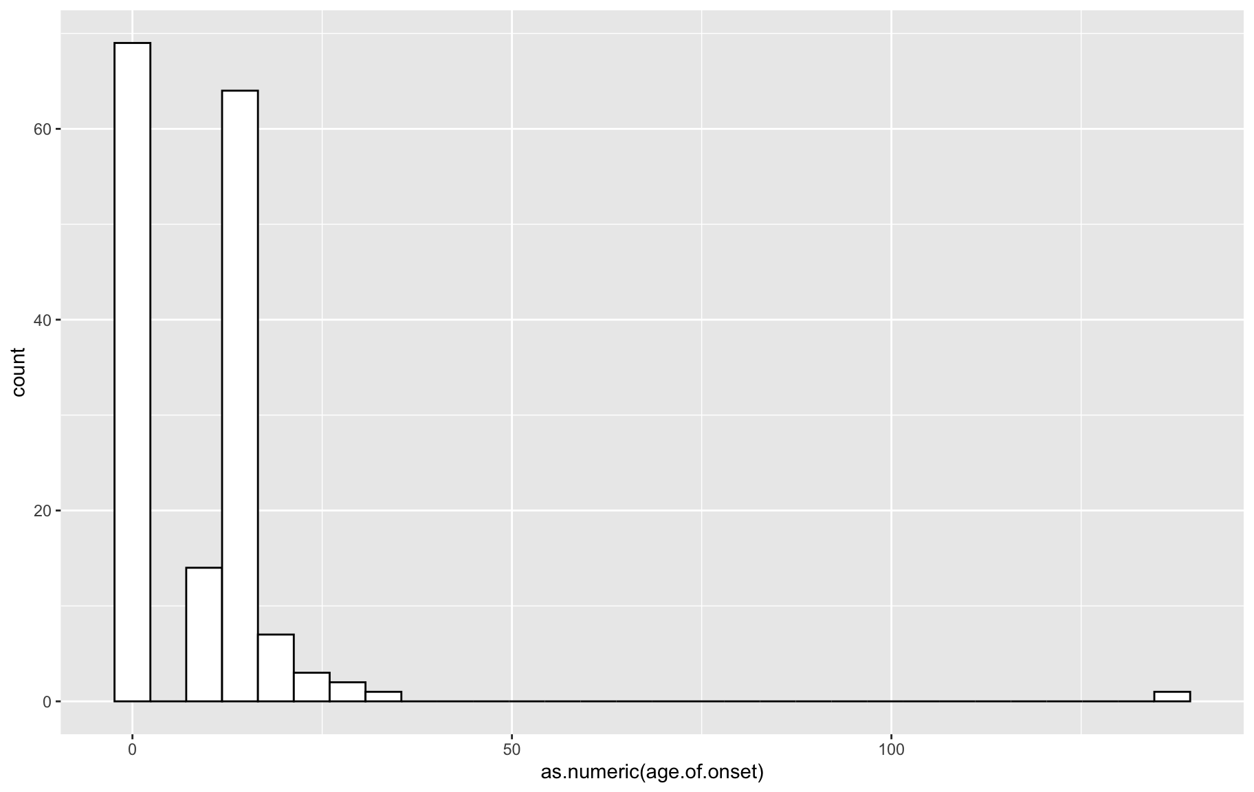
phenos.covars.lg <- gm$covar %>% gather(variable, value, -c("id","group","sex","diabetic status","strain","ICI.vs.EOI"))
box1 <- ggplot(data=phenos.covars.lg, aes(x=variable, y=as.numeric(value), color=group, fill=group)) +
geom_boxplot(position = position_dodge(width=0.9)) +
#ggtitle(paste0("Values of ",v," [random dataframe: ",r,"]")) +
#labs(y = v) +
theme(strip.text.x = element_text(size=13),
axis.text.x = element_text(size = 13, angle = 0),
axis.text.y = element_text(size = 13, angle = 0),
axis.title.x=element_blank(),
axis.title.y=element_blank(),
plot.title = element_text(size = 13, face = "bold",hjust = 0.5),
#legend.position = "none"
)
box1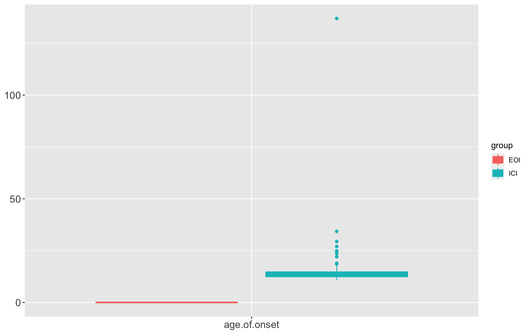 QTL analysis requires variables follow normal distribution, from the above distributions, we need to ranknorm the data.
##ranknorm
rz.transform <- function(y) {
  rankY=rank(y, ties.method="average", na.last="keep")
  rzT=qnorm(rankY/(length(na.exclude(rankY))+1))
  return(rzT)
}

gm$covar$rz.age <- rz.transform(gm$covar$age.of.onset)

p <- ggplot(gm$covar, aes(x=as.numeric(rz.age))) + geom_histogram(color="black", fill="white")
p
`stat_bin()` using `bins = 30`. Pick better value with `binwidth`.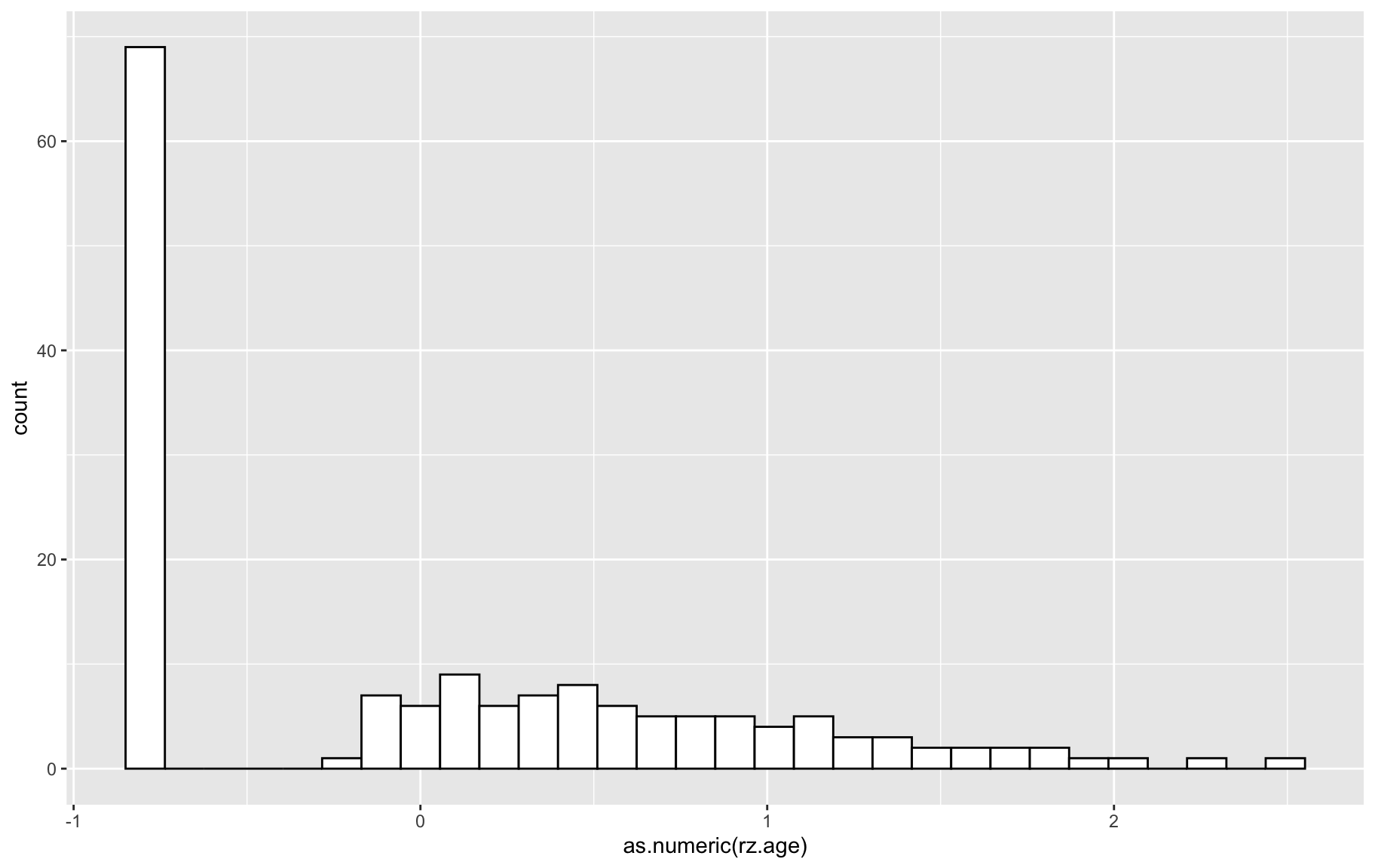
phenos.covars.lg <- gm$covar %>% gather(variable, value, -c("id","group","sex","diabetic status","strain","ICI.vs.EOI","age.of.onset"))

box1 <-  ggplot(data=phenos.covars.lg, aes(x=variable, y=as.numeric(value), color=group, fill=group)) +
         geom_boxplot(position = position_dodge(width=0.9)) +
         #ggtitle(paste0("Values of ",v," [random dataframe: ",r,"]")) +
         #labs(y = v) +
         theme(strip.text.x = element_text(size=13),
               axis.text.x = element_text(size = 13, angle = 0),
               axis.text.y = element_text(size = 13, angle = 0),
               axis.title.x=element_blank(),
               axis.title.y=element_blank(),
               plot.title = element_text(size = 13, face = "bold",hjust = 0.5),
                  #legend.position = "none"
             )
box1
And then remove any samples that are 3 standard deviations from the mean.
#outliers
#des.3 <- Hmisc::describe(df_phenos[,c("R_AVG","L_AVG","Both_AVG")])
des.1 <- pastecs::stat.desc(gm$covar[,c("age.of.onset" ,"rz.age")])
des.2 <- psych::describe(gm$covar[,c("age.of.onset" ,"rz.age")])

#scale(df_phenos[,c("R_AVG")])

gm$covar$out.age.of.onset <- ifelse(gm$covar[,c("age.of.onset")] > (des.1[9,1] + 3*des.1[13,1])  | gm$covar[,c("age.of.onset")] < (des.1[9,1] - 3*des.1[13,1]), 'Outlier','Keep')
gm$covar$out.rz.age <- ifelse(gm$covar[,c("rz.age")] > (des.1[9,2] + 3*des.1[13,2])  | gm$covar[,c("rz.age")] < (des.1[9,2] - 3*des.1[13,2]), 'Outlier','Keep')

bad <- NULL
bad$Mouse.ID <- rownames(gm$covar)
bad$age.of.onset <- ifelse(gm$covar$out.age.of.onset =="Outlier", 'XX', '')
bad$rz.age <- ifelse(gm$covar$out.rz.age =="Outlier", 'XX', '')
bad[is.na(bad)] <- ""
bad[bad=='NA'] <- ""
df <- do.call(cbind, bad)
bad <- as.data.frame(df)

badind <- subset(bad,
         bad$age.of.onset == 'XX'|
         bad$rz.age == 'XX')


#badind <- bad[bad$no_pheno == 'XX',]

badind[] <- lapply(badind, as.character)
#badind$Thaiss_ID <- ifelse(badind$Thaiss == 994 | badind$Thaiss == 995 | badind$Thaiss == 996 |badind$Thaiss == 997 | badind$Thaiss == 998 | badind$Thaiss == 999, "--", bad$Thaiss_ID)

rownames(badind) <- NULL

badind[] %>%
   dplyr::mutate(
     age.of.onset = ifelse(age.of.onset == 'XX',
                  cell_spec(age.of.onset, color = 'gray',background = 'gray'),
                  ''),
     rz.age = ifelse(rz.age == 'XX',
                  cell_spec(rz.age, color = 'gray',background = 'gray'),
                  '')
     ) %>%
   kable(escape = F,align = c("ccccccccc"),linesep ="\\hline") %>%
   kable_styling("striped", full_width = F) %>%
column_spec(1:3, width = "3cm") | Mouse.ID | age.of.onset | rz.age |
|---|---|---|
| NG00453 | XX |
##removing outliers
gm$covar$Mouse.ID <- rownames(gm$covar)
gm$covar$age.of.onset[gm$covar$out.age.of.onset == "Outlier"] <- ''
gm$covar$rz.age[gm$covar$out.rz.age == "Outlier"] <- ''

#gm$covar <- gm$covar[c(1:15)]
#gm$covar$id <- rownames(gm$covar)
write.csv(gm$covar,"data/covar_cleaned_ici.vs.eoi.csv", row.names=F, quote=F)
That is, those that have a grey square were removed for that particular phenotype in the QTL mapping.
ICI vs PBS
gm=gm_allqc

##extracting animals with ici and eoi group status
miceinfo <- gm$covar[gm$covar$group == "PBS" | gm$covar$group == "ICI",]
table(miceinfo$group)
ICI PBS
 92  21
mice.ids <- rownames(miceinfo)
gm <- gm[mice.ids]
gmObject of class cross2 (crosstype "bc")
Total individuals 113
No. genotyped individuals 113
No. phenotyped individuals 113
No. with both geno & pheno 113
No. phenotypes 1
No. covariates 6
No. phenotype covariates 0
No. chromosomes 20
Total markers 131578
No. markers by chr:
1 2 3 4 5 6 7 8 9 10 11 12 13
9977 10005 7858 7589 7621 7758 7413 6472 6725 6396 7154 6137 6085
14 15 16 17 18 19 X
5981 5346 5019 5093 4607 3564 4778 pr.qc <- pr
for (i in 1:20){pr.qc[[i]] = pr.qc[[i]][mice.ids,,]}
gm$covar$ICI.vs.PBS <- ifelse(gm$covar$group == "PBS", 0, 1)
names(gm$covar)[3] <- c("age.of.onset")
gm$covar$age.of.onset <- as.numeric(gm$covar$age.of.onset)
p <- ggplot(gm$covar, aes(x=as.numeric(age.of.onset))) + geom_histogram(color="black", fill="white")
p`stat_bin()` using `bins = 30`. Pick better value with `binwidth`.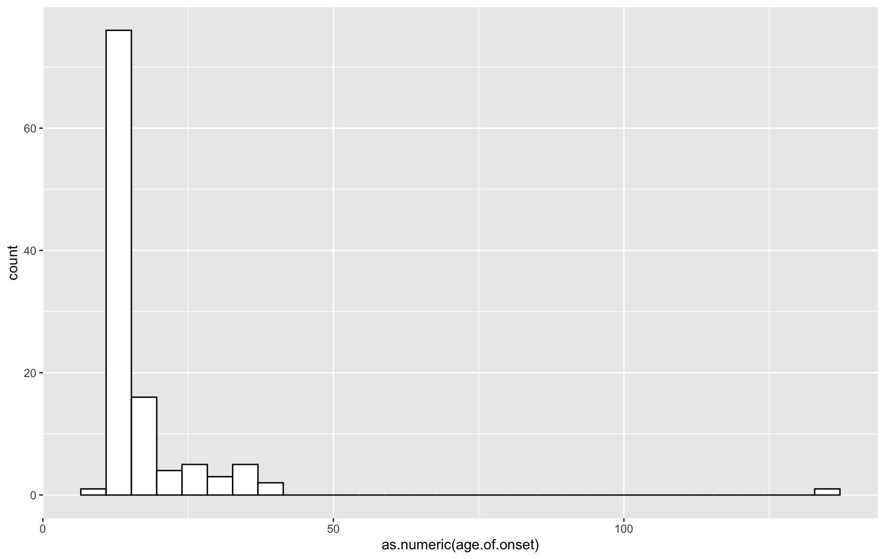
phenos.covars.lg <- gm$covar %>% gather(variable, value, -c("id","group","sex","diabetic status","strain","ICI.vs.PBS"))
box1 <- ggplot(data=phenos.covars.lg, aes(x=variable, y=as.numeric(value), color=group, fill=group)) +
geom_boxplot(position = position_dodge(width=0.9)) +
#ggtitle(paste0("Values of ",v," [random dataframe: ",r,"]")) +
#labs(y = v) +
theme(strip.text.x = element_text(size=13),
axis.text.x = element_text(size = 13, angle = 0),
axis.text.y = element_text(size = 13, angle = 0),
axis.title.x=element_blank(),
axis.title.y=element_blank(),
plot.title = element_text(size = 13, face = "bold",hjust = 0.5),
#legend.position = "none"
)
box1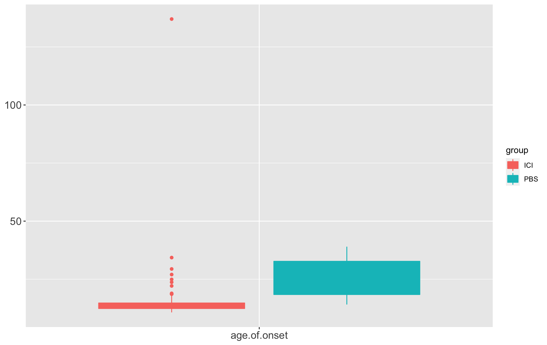 QTL analysis requires variables follow normal distribution, from the above distributions, we need to ranknorm the data.
##ranknorm
rz.transform <- function(y) {
  rankY=rank(y, ties.method="average", na.last="keep")
  rzT=qnorm(rankY/(length(na.exclude(rankY))+1))
  return(rzT)
}

gm$covar$rz.age <- rz.transform(gm$covar$age.of.onset)

p <- ggplot(gm$covar, aes(x=as.numeric(rz.age))) + geom_histogram(color="black", fill="white")
p
`stat_bin()` using `bins = 30`. Pick better value with `binwidth`.
phenos.covars.lg <- gm$covar %>% gather(variable, value, -c("id","group","sex","diabetic status","strain","ICI.vs.PBS","age.of.onset"))

box1 <-  ggplot(data=phenos.covars.lg, aes(x=variable, y=as.numeric(value), color=group, fill=group)) +
         geom_boxplot(position = position_dodge(width=0.9)) +
         #ggtitle(paste0("Values of ",v," [random dataframe: ",r,"]")) +
         #labs(y = v) +
         theme(strip.text.x = element_text(size=13),
               axis.text.x = element_text(size = 13, angle = 0),
               axis.text.y = element_text(size = 13, angle = 0),
               axis.title.x=element_blank(),
               axis.title.y=element_blank(),
               plot.title = element_text(size = 13, face = "bold",hjust = 0.5),
                  #legend.position = "none"
             )
box1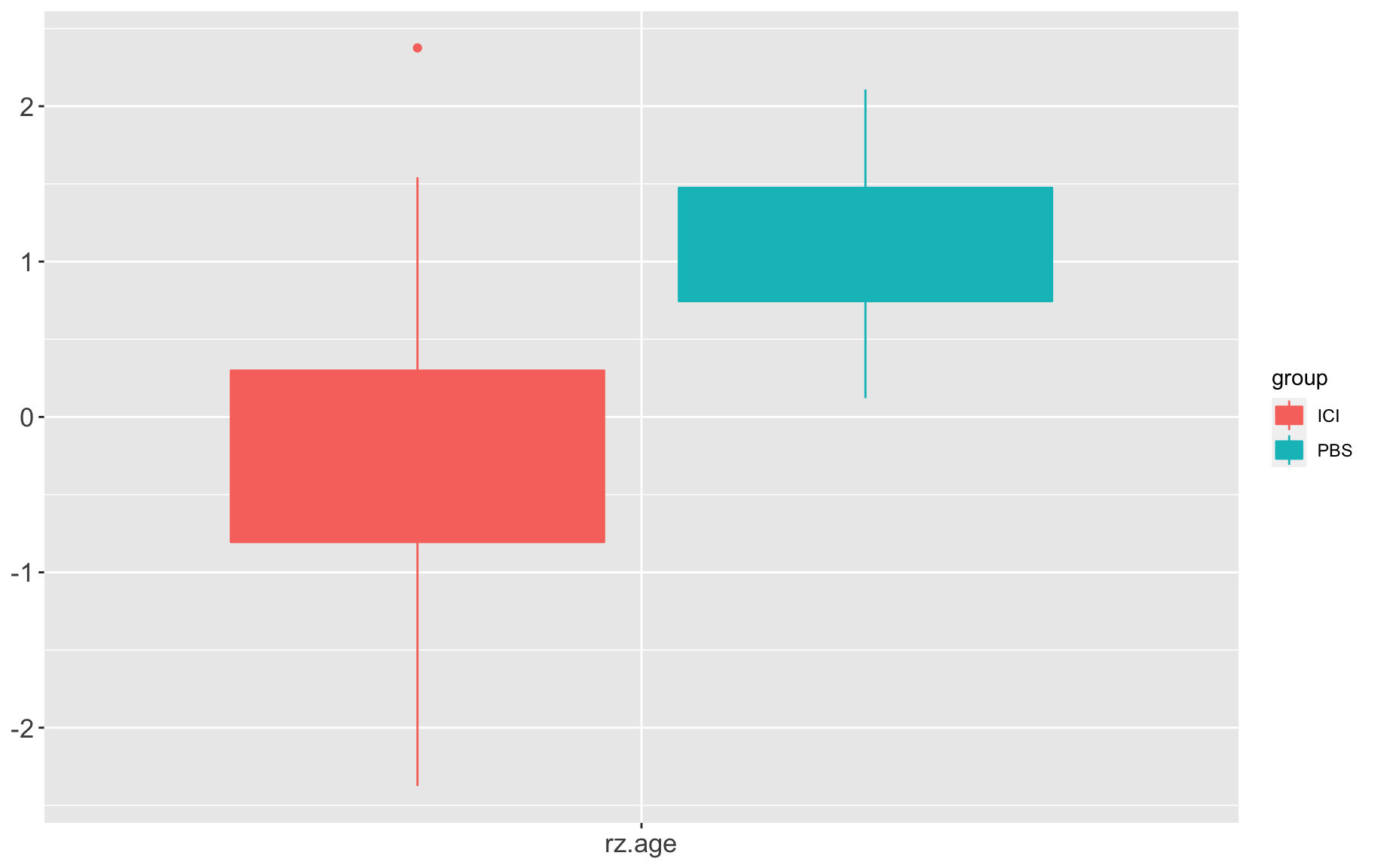
And then remove any samples that are 3 standard deviations from the mean.
#outliers
#des.3 <- Hmisc::describe(df_phenos[,c("R_AVG","L_AVG","Both_AVG")])
des.1 <- pastecs::stat.desc(gm$covar[,c("age.of.onset" ,"rz.age")])
des.2 <- psych::describe(gm$covar[,c("age.of.onset" ,"rz.age")])

#scale(df_phenos[,c("R_AVG")])

gm$covar$out.age.of.onset <- ifelse(gm$covar[,c("age.of.onset")] > (des.1[9,1] + 3*des.1[13,1])  | gm$covar[,c("age.of.onset")] < (des.1[9,1] - 3*des.1[13,1]), 'Outlier','Keep')
gm$covar$out.rz.age <- ifelse(gm$covar[,c("rz.age")] > (des.1[9,2] + 3*des.1[13,2])  | gm$covar[,c("rz.age")] < (des.1[9,2] - 3*des.1[13,2]), 'Outlier','Keep')

bad <- NULL
bad$Mouse.ID <- rownames(gm$covar)
bad$age.of.onset <- ifelse(gm$covar$out.age.of.onset =="Outlier", 'XX', '')
bad$rz.age <- ifelse(gm$covar$out.rz.age =="Outlier", 'XX', '')
bad[is.na(bad)] <- ""
bad[bad=='NA'] <- ""
df <- do.call(cbind, bad)
bad <- as.data.frame(df)

badind <- subset(bad,
         bad$age.of.onset == 'XX'|
         bad$rz.age == 'XX')


#badind <- bad[bad$no_pheno == 'XX',]

badind[] <- lapply(badind, as.character)
#badind$Thaiss_ID <- ifelse(badind$Thaiss == 994 | badind$Thaiss == 995 | badind$Thaiss == 996 |badind$Thaiss == 997 | badind$Thaiss == 998 | badind$Thaiss == 999, "--", bad$Thaiss_ID)

rownames(badind) <- NULL

badind[] %>%
   dplyr::mutate(
     age.of.onset = ifelse(age.of.onset == 'XX',
                  cell_spec(age.of.onset, color = 'gray',background = 'gray'),
                  ''),
     rz.age = ifelse(rz.age == 'XX',
                  cell_spec(rz.age, color = 'gray',background = 'gray'),
                  '')
     ) %>%
   kable(escape = F,align = c("ccccccccc"),linesep ="\\hline") %>%
   kable_styling("striped", full_width = F) %>%
column_spec(1:3, width = "3cm") | Mouse.ID | age.of.onset | rz.age |
|---|---|---|
| NG00453 | XX |
##removing outliers
gm$covar$Mouse.ID <- rownames(gm$covar)
gm$covar$age.of.onset[gm$covar$out.age.of.onset == "Outlier"] <- ''
gm$covar$rz.age[gm$covar$out.rz.age == "Outlier"] <- ''

#gm$covar <- gm$covar[c(1:15)]
#gm$covar$id <- rownames(gm$covar)
write.csv(gm$covar,"data/covar_cleaned_ici.vs.pbs.csv", row.names=F, quote=F)
That is, those that have a grey square were removed for that particular phenotype in the QTL mapping.
R version 3.6.2 (2019-12-12)
Platform: x86_64-apple-darwin15.6.0 (64-bit)
Running under: macOS Catalina 10.15.7

Matrix products: default
BLAS:   /Library/Frameworks/R.framework/Versions/3.6/Resources/lib/libRblas.0.dylib
LAPACK: /Library/Frameworks/R.framework/Versions/3.6/Resources/lib/libRlapack.dylib

locale:
[1] en_AU.UTF-8/en_AU.UTF-8/en_AU.UTF-8/C/en_AU.UTF-8/en_AU.UTF-8

attached base packages:
[1] stats     graphics  grDevices utils     datasets  methods   base

other attached packages:
 [1] abind_1.4-5       qtl2_0.22         reshape2_1.4.4    ggplot2_3.3.5
 [5] tibble_3.1.2      psych_2.0.7       readxl_1.3.1      cluster_2.1.0
 [9] dplyr_0.8.5       optparse_1.6.6    rhdf5_2.28.1      mclust_5.4.6
[13] tidyr_1.0.2       data.table_1.14.0 knitr_1.33        kableExtra_1.1.0
[17] workflowr_1.6.2

loaded via a namespace (and not attached):
 [1] httr_1.4.1        bit64_4.0.5       viridisLite_0.4.0 assertthat_0.2.1
 [5] highr_0.9         blob_1.2.1        cellranger_1.1.0  yaml_2.2.1
 [9] pillar_1.6.1      RSQLite_2.2.7     backports_1.2.1   lattice_0.20-38
[13] glue_1.4.2        digest_0.6.27     promises_1.1.0    rvest_0.3.5
[17] colorspace_2.0-2  htmltools_0.5.1.1 httpuv_1.5.2      plyr_1.8.6
[21] pkgconfig_2.0.3   purrr_0.3.4       scales_1.1.1      webshot_0.5.2
[25] whisker_0.4       getopt_1.20.3     later_1.0.0       git2r_0.26.1
[29] farver_2.1.0      ellipsis_0.3.2    cachem_1.0.5      withr_2.4.2
[33] mnormt_1.5-7      magrittr_2.0.1    crayon_1.4.1      memoise_2.0.0
[37] evaluate_0.14     fs_1.4.1          fansi_0.5.0       nlme_3.1-142
[41] xml2_1.3.1        tools_3.6.2       hms_0.5.3         lifecycle_1.0.0
[45] stringr_1.4.0     Rhdf5lib_1.6.3    munsell_0.5.0     pastecs_1.3.21
[49] compiler_3.6.2    rlang_0.4.11      grid_3.6.2        rstudioapi_0.13
[53] labeling_0.4.2    rmarkdown_2.1     boot_1.3-23       gtable_0.3.0
[57] DBI_1.1.1         R6_2.5.0          fastmap_1.1.0     bit_4.0.4
[61] utf8_1.2.1        rprojroot_1.3-2   readr_1.3.1       stringi_1.7.2
[65] parallel_3.6.2    Rcpp_1.0.7        vctrs_0.3.8       tidyselect_1.0.0
[69] xfun_0.24