QTL Analysis - binary [ICI vs PBS]

Data Information
Loading Data
Genome-wide scan
LOD peaks
QTL effects

Last updated: 2022-03-15

Checks: 6 1

Knit directory: Serreze-T1D_Workflow/

This reproducible R Markdown analysis was created with workflowr (version 1.6.2). The Checks tab describes the reproducibility checks that were applied when the results were created. The Past versions tab lists the development history.

R Markdown file: up-to-date

Great! Since the R Markdown file has been committed to the Git repository, you know the exact version of the code that produced these results.

Environment: empty

Great job! The global environment was empty. Objects defined in the global environment can affect the analysis in your R Markdown file in unknown ways. For reproduciblity it’s best to always run the code in an empty environment.

Seed: set.seed(20220210)

The command set.seed(20220210) was run prior to running the code in the R Markdown file. Setting a seed ensures that any results that rely on randomness, e.g. subsampling or permutations, are reproducible.

Session information: recorded

Great job! Recording the operating system, R version, and package versions is critical for reproducibility.

Cache: none

Nice! There were no cached chunks for this analysis, so you can be confident that you successfully produced the results during this run.

File paths: absolute

Using absolute paths to the files within your workflowr project makes it difficult for you and others to run your code on a different machine. Change the absolute path(s) below to the suggested relative path(s) to make your code more reproducible.

absolute	relative
/Users/corneb/Documents/MyJax/CS/Projects/Serreze/qc/workflowr/Serreze-T1D_Workflow	.

Repository version: 93afca9

Great! You are using Git for version control. Tracking code development and connecting the code version to the results is critical for reproducibility.

The results in this page were generated with repository version 93afca9. See the Past versions tab to see a history of the changes made to the R Markdown and HTML files.

Note that you need to be careful to ensure that all relevant files for the analysis have been committed to Git prior to generating the results (you can use wflow_publish or wflow_git_commit). workflowr only checks the R Markdown file, but you know if there are other scripts or data files that it depends on. Below is the status of the Git repository when the results were generated:


Ignored files:
    Ignored:    .DS_Store
    Ignored:    analysis/.DS_Store

Untracked files:
    Untracked:  data/GM_covar.csv
    Untracked:  data/bad_markers_all_4.batches.RData
    Untracked:  data/covar_cleaned_ici.vs.eoi.csv
    Untracked:  data/covar_cleaned_ici.vs.pbs.csv
    Untracked:  data/covar_corrected.cleaned_ici.vs.eoi.csv
    Untracked:  data/covar_corrected.cleaned_ici.vs.eoi1.csv
    Untracked:  data/covar_corrected.cleaned_ici.vs.pbs.csv
    Untracked:  data/covar_corrected.cleaned_ici.vs.pbs1.csv
    Untracked:  data/covar_corrected_ici.vs.eoi.csv
    Untracked:  data/covar_corrected_ici.vs.eoi1.csv
    Untracked:  data/covar_corrected_ici.vs.pbs.csv
    Untracked:  data/covar_corrected_ici.vs.pbs1.csv
    Untracked:  data/e.RData
    Untracked:  data/e_snpg_samqc_4.batches.RData
    Untracked:  data/e_snpg_samqc_4.batches_bc.RData
    Untracked:  data/errors_ind_4.batches.RData
    Untracked:  data/errors_ind_4.batches_bc.RData
    Untracked:  data/genetic_map.csv
    Untracked:  data/genotype_errors_marker_4.batches.RData
    Untracked:  data/genotype_freq_marker_4.batches.RData
    Untracked:  data/gm_allqc_4.batches.RData
    Untracked:  data/gm_samqc_3.batches.RData
    Untracked:  data/gm_samqc_4.batches.RData
    Untracked:  data/gm_samqc_4.batches_bc.RData
    Untracked:  data/gm_serreze.192.RData
    Untracked:  data/ici.vs.eoi_marker.freq_low.geno.freq.removed_geno.ratio.csv
    Untracked:  data/ici.vs.eoi_marker.freq_low.geno.freq.removed_sample.outliers.removed_geno.ratio.csv
    Untracked:  data/ici.vs.eoi_marker.freq_low.probs.freq.removed_geno.ratio.csv
    Untracked:  data/ici.vs.eoi_marker.freq_low.probs.freq.removed_sample.outliers.removed_geno.ratio.csv
    Untracked:  data/ici.vs.eoi_sample.genos_marker.freq_low.geno.freq.removed.csv
    Untracked:  data/ici.vs.eoi_sample.genos_marker.freq_low.geno.freq.removed_sample.outliers.removed.csv
    Untracked:  data/ici.vs.eoi_sample.genos_marker.freq_low.probs.freq.removed.csv
    Untracked:  data/ici.vs.eoi_sample.genos_marker.freq_low.probs.freq.removed_sample.outliers.removed.csv
    Untracked:  data/ici.vs.pbs_marker.freq_low.geno.freq.removed_geno.ratio.csv
    Untracked:  data/ici.vs.pbs_marker.freq_low.geno.freq.removed_sample.outliers.removed_geno.ratio.csv
    Untracked:  data/ici.vs.pbs_marker.freq_low.probs.freq.removed_geno.ratio.csv
    Untracked:  data/ici.vs.pbs_marker.freq_low.probs.freq.removed_sample.outliers.removed_geno.ratio.csv
    Untracked:  data/ici.vs.pbs_sample.genos_marker.freq_low.geno.freq.removed.csv
    Untracked:  data/ici.vs.pbs_sample.genos_marker.freq_low.geno.freq.removed_sample.outliers.removed.csv
    Untracked:  data/ici.vs.pbs_sample.genos_marker.freq_low.probs.freq.removed.csv
    Untracked:  data/ici.vs.pbs_sample.genos_marker.freq_low.probs.freq.removed_sample.outliers.removed.csv
    Untracked:  data/percent_missing_id_3.batches.RData
    Untracked:  data/percent_missing_id_4.batches.RData
    Untracked:  data/percent_missing_id_4.batches_bc.RData
    Untracked:  data/percent_missing_marker_4.batches.RData
    Untracked:  data/pheno.csv
    Untracked:  data/physical_map.csv
    Untracked:  data/qc_info_bad_sample_3.batches.RData
    Untracked:  data/qc_info_bad_sample_4.batches.RData
    Untracked:  data/qc_info_bad_sample_4.batches_bc.RData
    Untracked:  data/remaining.markers_geno.freq.xlsx
    Untracked:  data/sample_geno.csv
    Untracked:  data/sample_geno_bc.csv
    Untracked:  data/serreze_probs.rds
    Untracked:  data/serreze_probs_allqc.rds
    Untracked:  data/summary.cg_3.batches.RData
    Untracked:  data/summary.cg_4.batches.RData
    Untracked:  data/summary.cg_4.batches_bc.RData

Note that any generated files, e.g. HTML, png, CSS, etc., are not included in this status report because it is ok for generated content to have uncommitted changes.

These are the previous versions of the repository in which changes were made to the R Markdown (analysis/4.1.1_qtl.analysis_binary_ici.vs.pbs_snpsqc_dis_no-x_updated.Rmd) and HTML (docs/4.1.1_qtl.analysis_binary_ici.vs.pbs_snpsqc_dis_no-x_updated.html) files. If you’ve configured a remote Git repository (see ?wflow_git_remote), click on the hyperlinks in the table below to view the files as they were in that past version.

File	Version	Author	Date	Message
Rmd	93afca9	Belinda Cornes	2022-03-15	updated binary qtl

Data Information

binary phenotype (therefore no kinship)
no Xcovar
low frequency (< 5% in samples) removed
disproportionate markers removed

Loading Data

We will load the data and subset indivials out that are in the groups of interest. We will create a binary phenotype from this (PBS ==0, ICI == 1).

load("data/gm_allqc_4.batches.RData")

#gm_allqc
gm=gm_allqc
gm

Object of class cross2 (crosstype "bc")

Total individuals               188
No. genotyped individuals       188
No. phenotyped individuals      188
No. with both geno & pheno      188

No. phenotypes                    1
No. covariates                    6
No. phenotype covariates          0

No. chromosomes                  20
Total markers                131578

No. markers by chr:
    1     2     3     4     5     6     7     8     9    10    11    12    13 
 9977 10005  7858  7589  7621  7758  7413  6472  6725  6396  7154  6137  6085 
   14    15    16    17    18    19     X 
 5981  5346  5019  5093  4607  3564  4778

#pr <- readRDS("data/serreze_probs_allqc.rds")
#pr <- readRDS("data/serreze_probs.rds")

##extracting animals with ici and pbs group status
miceinfo <- gm$covar[gm$covar$group == "PBS" | gm$covar$group == "ICI",]
table(miceinfo$group)


ICI PBS 
 92  21

mice.ids <- rownames(miceinfo)

gm <- gm[mice.ids]
gm

Object of class cross2 (crosstype "bc")

Total individuals               113
No. genotyped individuals       113
No. phenotyped individuals      113
No. with both geno & pheno      113

No. phenotypes                    1
No. covariates                    6
No. phenotype covariates          0

No. chromosomes                  20
Total markers                131578

No. markers by chr:
    1     2     3     4     5     6     7     8     9    10    11    12    13 
 9977 10005  7858  7589  7621  7758  7413  6472  6725  6396  7154  6137  6085 
   14    15    16    17    18    19     X 
 5981  5346  5019  5093  4607  3564  4778

table(gm$covar$group)


ICI PBS 
 92  21

gm$covar$ICI.vs.PBS <- ifelse(gm$covar$group == "PBS", 0, 1)

covars <- read_csv("data/covar_corrected.cleaned_ici.vs.pbs.csv")
#removing any missing info
covars <- subset(covars, covars$ICI.vs.PBS!='')
nrow(covars)

[1] 113

table(covars$group)


ICI PBS 
 92  21

#keeping only informative mice
gm <- gm[covars$Mouse.ID]
gm

Object of class cross2 (crosstype "bc")

Total individuals               113
No. genotyped individuals       113
No. phenotyped individuals      113
No. with both geno & pheno      113

No. phenotypes                    1
No. covariates                    7
No. phenotype covariates          0

No. chromosomes                  20
Total markers                131578

No. markers by chr:
    1     2     3     4     5     6     7     8     9    10    11    12    13 
 9977 10005  7858  7589  7621  7758  7413  6472  6725  6396  7154  6137  6085 
   14    15    16    17    18    19     X 
 5981  5346  5019  5093  4607  3564  4778

table(gm$covar$group)


ICI PBS 
 92  21

#pr.qc.ids <- pr
#for (i in 1:20){pr.qc.ids[[i]] = pr.qc.ids[[i]][covars$Mouse.ID,,]}


##dropping monomorphic markers within the dataset

g <- do.call("cbind", gm$geno)

gf_mar <- t(apply(g, 2, function(a) table(factor(a, 1:2))/sum(a != 0)))
#gn_mar <- t(apply(g, 2, function(a) table(factor(a, 1:2))))

gf_mar <- gf_mar[gf_mar[,2] != "NaN",]

count <- rowSums(gf_mar <=0.05)
low_freq_df <- merge(as.data.frame(gf_mar),as.data.frame(count), by="row.names",all=T)
low_freq_df[is.na(low_freq_df)] <- ''
low_freq_df <- low_freq_df[low_freq_df$count == 1,]
rownames(low_freq_df) <- low_freq_df$Row.names

low_freq <- find_markerpos(gm, rownames(low_freq_df))
low_freq$id <- rownames(low_freq)

nrow(low_freq)

[1] 98210

low_freq_bad <- merge(low_freq,low_freq_df, by="row.names",all=T)
names(low_freq_bad)[1] <- c("marker")

gf_mar <- gf_mar[gf_mar[,2] != "NaN",]
MAF <- apply(gf_mar, 1, function(x) min(x))
MAF <- as.data.frame(MAF)
MAF$index <- 1:nrow(gf_mar)
gf_mar_maf <- merge(gf_mar,as.data.frame(MAF), by="row.names")
gf_mar_maf <- gf_mar_maf[order(gf_mar_maf$index),]

gfmar <- NULL
gfmar$gfmar_mar_0 <- sum(gf_mar_maf$MAF==0)
gfmar$gfmar_mar_1 <- sum(gf_mar_maf$MAF< 0.01)
gfmar$gfmar_mar_5 <- sum(gf_mar_maf$MAF< 0.05)
gfmar$gfmar_mar_10 <- sum(gf_mar_maf$MAF< 0.10)
gfmar$gfmar_mar_15 <- sum(gf_mar_maf$MAF< 0.15)
gfmar$gfmar_mar_25 <- sum(gf_mar_maf$MAF< 0.25)
gfmar$gfmar_mar_50 <- sum(gf_mar_maf$MAF< 0.50)
gfmar$total_snps <- nrow(as.data.frame(gf_mar_maf))

gfmar <- t(as.data.frame(gfmar))
gfmar <- as.data.frame(gfmar)
gfmar$count <- gfmar$V1

gfmar[c(2)] %>%
  kable(escape = F,align = c("ccccccccc"),linesep ="\\hline") %>%
  kable_styling(full_width = F) %>%
  kable_styling("striped", full_width = F)  %>%
  row_spec(8 ,bold=T,color= "white",background = "black")

	count
gfmar_mar_0	89064
gfmar_mar_1	92616
gfmar_mar_5	98209
gfmar_mar_10	99489
gfmar_mar_15	99575
gfmar_mar_25	100325
gfmar_mar_50	131283
total_snps	131578

gm_qc <- drop_markers(gm, low_freq_bad$marker)
gm_qc <- drop_nullmarkers(gm_qc)

gm_qc

Object of class cross2 (crosstype "bc")

Total individuals              113
No. genotyped individuals      113
No. phenotyped individuals     113
No. with both geno & pheno     113

No. phenotypes                   1
No. covariates                   7
No. phenotype covariates         0

No. chromosomes                 20
Total markers                33368

No. markers by chr:
   1    2    3    4    5    6    7    8    9   10   11   12   13   14   15   16 
3009 2925 2089 2103 1982 2099 1915 1739 2050 1253 2102 1428 1656 1728 1101  977 
  17   18   19    X 
 422 1118 1084  588

## dropping disproportionate markers
dismark <- read.csv("data/ici.vs.pbs_marker.freq_low.geno.freq.removed_geno.ratio.csv")
nrow(dismark)

[1] 33368

names(dismark)[1] <- c("marker")
dismark <- dismark[!dismark$Include,]
nrow(dismark)

[1] 24442

gm_qc_dis <- drop_markers(gm_qc, dismark$marker)
gm_qc_dis <- drop_nullmarkers(gm_qc_dis)

gm = gm_qc_dis
gm

Object of class cross2 (crosstype "bc")

Total individuals             113
No. genotyped individuals     113
No. phenotyped individuals    113
No. with both geno & pheno    113

No. phenotypes                  1
No. covariates                  7
No. phenotype covariates        0

No. chromosomes                19
Total markers                8926

No. markers by chr:
   1    2    3    4    5    6    7    8    9   10   11   12   13   14   16   17 
 281 1238    5  177  775  979  558  220  394  146  554  308  307  899  203    2 
  18   19    X 
 867  688  325

markers <- marker_names(gm)
gmapdf <- read.csv("/Users/corneb/Documents/MyJax/CS/Projects/Serreze/haplotype.reconstruction/output_hh/genetic_map.csv")
pmapdf <- read.csv("/Users/corneb/Documents/MyJax/CS/Projects/Serreze/haplotype.reconstruction/output_hh/physical_map.csv")
mapdf <- merge(gmapdf,pmapdf, by=c("marker","chr"), all=T)
rownames(mapdf) <- mapdf$marker
mapdf <- mapdf[markers,]
names(mapdf) <- c('marker','chr','gmapdf','pmapdf')
mapdfnd <- mapdf[!duplicated(mapdf[c(2:3)]),]

pr.qc <- calc_genoprob(gm)

Genome-wide scan

For each of the phenotype analyzed, permutations were used for each model to obtain genome-wide LOD significance threshold for p < 0.01, p < 0.05, p < 0.10, respectively, separately for X and automsomes (A).

The table shows the estimated significance thresholds from permutation test.

We also looked at the kinship to see how correlated each sample is. Kinship values between pairs of samples range between 0 (no relationship) and 1.0 (completely identical). The darker the colour the more indentical the pairs are.

#Xcovar <- get_x_covar(gm)
#addcovar = model.matrix(~Sex, data = covars)[,-1]

#K <- calc_kinship(pr.qc, type = "loco")
#heatmap(K[[1]])
#K.overall <- calc_kinship(pr.qc, type = "overall")
#heatmap(K.overall)
kinship <- calc_kinship(pr.qc)
heatmap(kinship)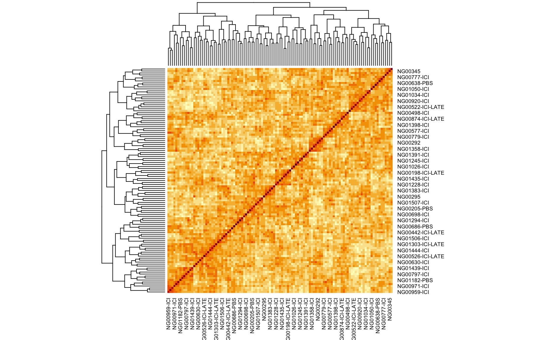

#operm <- scan1perm(pr.qc, gm$covar$phenos, Xcovar=Xcovar, n_perm=2000)
#operm <- scan1perm(pr.qc, gm$covar$phenos, addcovar = addcovar, n_perm=2000)
#operm <- scan1perm(pr.qc, gm$covar$phenos, n_perm=2000)
operm <- scan1perm(pr.qc, gm$covar["ICI.vs.PBS"], model="binary", n_perm=1000, perm_Xsp=TRUE, chr_lengths=chr_lengths(gm$gmap))

summary_table<-data.frame(unclass(summary(operm, alpha=c(0.01,  0.05, 0.1))))
names(summary_table) <- c("autosomes","X")
summary_table$significance.level <- rownames(summary_table)

rownames(summary_table) <- NULL

summary_table[c(3,1:2)] %>%
  kable(escape = F,align = c("ccc")) %>%
  kable_styling("striped", full_width = T) %>%
  column_spec(1, bold=TRUE)

significance.level	autosomes	X
0.01	3.612485	3.433133
0.05	2.971605	3.186335
0.1	2.725731	2.725117

The figures below show QTL maps for each phenotype

#out <- scan1(pr.qc, gm$covar["ICI.vs.PBS"], Xcovar=Xcovar, model="binary")
out <- scan1(pr.qc, gm$covar["ICI.vs.PBS"], model="binary")

summary_table<-data.frame(unclass(summary(operm, alpha=c(0.01,  0.05, 0.1))))

plot_lod<-function(out,map){
  for (i in 1:dim(out)[2]){
    #png(filename=paste0("/Users/chenm/Documents/qtl/Jai/",colnames(out)[i],  "_lod.png"))
    
    #par(mar=c(5.1, 6.1, 1.1, 1.1))
    ymx <- 6 # overall maximum LOD score
    plot(out, map, lodcolumn=i, col="slateblue", ylim=c(0, ymx+0.5))
    legend("topright", lwd=2, colnames(out)[i], bg="gray90")
    title(main = paste0(colnames(out)[i], " [positions in cM]"))
    add_threshold(map,  summary(operm,alpha=0.1), col = 'purple')
    add_threshold(map,  summary(operm, alpha=0.05), col = 'red')
    add_threshold(map,  summary(operm, alpha=0.01), col = 'blue')
    #for (j in 1: dim(summary_table)[1]){
    #  abline(h=summary_table[j, i],col="red")
    #  text(x=400, y =summary_table[j, i]+0.12, labels = paste("p=", row.names(summary_table)[j]))
    #}
    #dev.off()
  }
}

plot_lod(out,gm$gmap)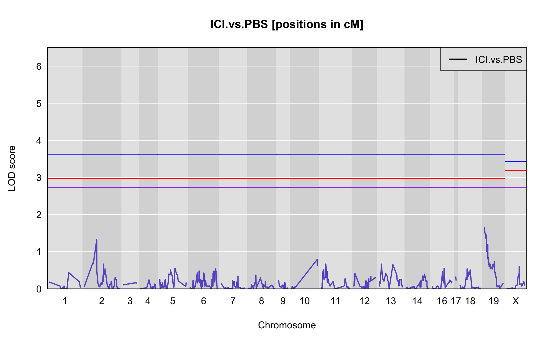

LOD peaks

The table below shows QTL peaks associated with the phenotype. We use the 95% threshold from the permutations to find peaks.

#peaks<-find_peaks(out, gm$gmap, threshold=3.6, drop=1.5, peakdrop=3)
#peaks <- find_peaks(out, gm$gmap,drop=1.5, peakdrop=3)
#peaks <- find_peaks(out, gm$gmap, threshold=3, peakdrop=1, drop=1)
#peaks <- find_peaks(out, gm$gmap, peakdrop=0.5, drop=0.5)
peaks <- find_peaks(out, gm$gmap, threshold=summary(operm,alpha=0.01)$A, thresholdX = summary(operm,alpha=0.01)$X, peakdrop=3, drop=1.5)

if(nrow(peaks) >0){
rownames(peaks) <- NULL
peaks[] %>%
  kable(escape = F,align = c("ccccccc")) %>%
  kable_styling("striped", full_width = T) %>%
  column_spec(1, bold=TRUE)

#plot only peak chromosomes

plot_lod_chr<-function(out,map,chrom){
  for (i in 1:dim(out)[2]){
    #png(filename=paste0("/Users/chenm/Documents/qtl/Jai/",colnames(out)[i],  "_lod.png"))
    
    #par(mar=c(5.1, 6.1, 1.1, 1.1))
    ymx <- maxlod(out) # overall maximum LOD score
    plot(out, map, chr = chrom, lodcolumn=i, col="slateblue", ylim=c(0, ymx+0.5))
    legend("topright", lwd=2, colnames(out)[i], bg="gray90")
    title(main = paste0(colnames(out)[i], " - chr", chrom, " [positions in cM]"))
    add_threshold(map,  summary(operm,alpha=0.1), col = 'purple')
    add_threshold(map,  summary(operm, alpha=0.05), col = 'red')
    add_threshold(map,  summary(operm, alpha=0.01), col = 'blue')
    #for (j in 1: dim(summary_table)[1]){
    #  abline(h=summary_table[j, i],col="red")
    #  text(x=400, y =summary_table[j, i]+0.12, labels = paste("p=", row.names(summary_table)[j]))
    #}
    #dev.off()
  }
}

for (i in 1:nrow(peaks)){
  plot_lod_chr(out,gm$gmap, peaks$chr[i])
}

peaks_mbl <- list()
#corresponding info in Mb
for(i in 1:nrow(peaks)){
  lodindex <- peaks$lodindex[i]
  lodcolumn <- peaks$lodcolumn[i]
  chr <- as.character(peaks$chr[i])
  lod <- peaks$lod[i]
  mark <- find_marker(gm$gmap, chr=chr,pos=peaks$pos[i])
  pos <- mapdf[mapdf$marker==mark,]$pmapdf
  ci_lo <- mapdfnd$pmapdf[which(mapdfnd$gmapdf == peaks$ci_lo[i] & mapdfnd$chr == peaks$chr[i])]
  ci_hi <- mapdfnd$pmapdf[which(mapdfnd$gmapdf == peaks$ci_hi[i] & mapdfnd$chr == peaks$chr[i])]
  peaks_mb=cbind(lodindex, lodcolumn, chr, pos, lod, ci_lo, ci_hi)
  peaks_mbl[[i]] <- peaks_mb
}
peaks_mba <- do.call(rbind, peaks_mbl)
peaks_mba <- as.data.frame(peaks_mba)
#peaks_mba[,c("chr", "pos", "lod", "ci_lo", "ci_hi")] <- sapply(peaks_mba[,c("chr", "pos", "lod", "ci_lo", "ci_hi")], as.numeric)

rownames(peaks_mba) <- NULL
peaks_mba[] %>%
  kable(escape = F,align = c("ccccccc")) %>%
  kable_styling("striped", full_width = T) %>%
  column_spec(1, bold=TRUE)

} else {
  print(paste0("There are no peaks that have a LOD that reaches significance (p<0.01) level of ",summary(operm,alpha=0.01)$A, " [autosomes]/",summary(operm,alpha=0.01)$X, " [x-chromosome]"))
}

[1] "There are no peaks that have a LOD that reaches significance (p<0.01) level of 3.61248459771541 [autosomes]/3.43313317528582 [x-chromosome]"

QTL effects

For each peak LOD location we give a list of gene

query_variants <- create_variant_query_func("/Users/corneb/Documents/MyJax/CS/Projects/support.files/qtl2/cc_variants.sqlite")
query_genes <- create_gene_query_func("/Users/corneb/Documents/MyJax/CS/Projects/support.files/qtl2/mouse_genes_mgi.sqlite")

if(nrow(peaks) >0){
for (i in 1:nrow(peaks)){
#for (i in 1:1){
  #Plot 1
  marker = find_marker(gm$gmap, chr=peaks$chr[i], pos=peaks$pos[i])
  #g <- maxmarg(pr.qc, gm$gmap, chr=peaks$chr[i], pos=peaks$pos[i], return_char=TRUE, minprob = 0.5)
  gp <- g[,marker]
  gp[gp==1] <- "AA"
  gp[gp==2] <- "AB"
  gp[gp==0] <- NA
  #png(filename=paste0("/Users/chenm/Documents/qtl/Jai/","qtl_effect_", i, ".png"))
  #par(mar=c(4.1, 4.1, 1.5, 0.6))
  plot_pxg(gp, gm$covar[,peaks$lodcolumn[i]], ylab=peaks$lodcolumn[i], sort=FALSE)
  title(main = paste("chr", chr=peaks$chr[i], "pos: ", peaks$pos[i], "cM /",peaks_mba$pos[i],"mb (",peaks$lodcolumn[i],")"), line=0.2)
  ##dev.off()

  chr = peaks$chr[i]

# Plot 2
  pr_sub <- pull_genoprobint(pr.qc, gm$gmap, chr, c(peaks$ci_lo[i], peaks$ci_hi[i]))
  #coeff <- scan1coef(pr[,chr], cross$pheno[,peaks$lodcolumn[i]], addcovar = addcovar)
  #coeff <- scan1coef(pr[,chr], cross$pheno[,peaks$lodcolumn[i]], Xcovar=Xcovar)
  #coeff <- scan1coef(pr.qc[,chr], gm$covar[peaks$lodcolumn[i]], model="binary")
  #coeff_sub <- scan1coef(pr_sub[,chr], gm$covar[peaks$lodcolumn[i]], model="binary")
  blup <- scan1blup(pr.qc[,chr], gm$covar[peaks$lodcolumn[i]])
  blup_sub <- scan1blup(pr_sub[,chr], gm$covar[peaks$lodcolumn[i]])

  #plot_coef(coeff, 
  #     gm$gmap, columns=1:2,
  #     bgcolor="gray95", legend="bottomleft", 
  #     main = paste("chr", chr=peaks$chr[i], "pos: ", peaks$pos[i], "cM /",peaks_mba$pos[i],"MB\n(",peaks$lodcolumn[i]," [scan1coeff; positions in cM] )")
  #     )

  #plot_coef(coeff_sub, 
  #     gm$gmap, columns=1:2,
  #     bgcolor="gray95", legend="bottomleft", 
  #     main = paste("chr", chr=peaks$chr[i], "pos: ", peaks$pos[i], "cM /",peaks_mba$pos[i],"MB\n(",peaks$lodcolumn[i],"; 1.5 LOD drop interval [scan1coeff; positions in cM] ) ")
  #     )


  plot_coef(blup, 
       gm$gmap, columns=1:2,
       bgcolor="gray95", legend="bottomleft", 
       main = paste("chr", chr=peaks$chr[i], "pos: ", peaks$pos[i], "cM /",peaks_mba$pos[i],"MB\n(",peaks$lodcolumn[i]," [scan1blup; positions in cM] )")
       )

  plot_coef(blup_sub, 
       gm$gmap, columns=1:2,
       bgcolor="gray95", legend="bottomleft", 
       main = paste("chr", chr=peaks$chr[i], "pos: ", peaks$pos[i], "cM /",peaks_mba$pos[i],"MB\n(",peaks$lodcolumn[i],"; 1.5 LOD drop interval [scan1blup; positions in cM] )")
       )

  #last_coef <- unclass(coeff)[nrow(coeff),1:3]
  #for(t in seq(along=last_coef))
  #axis(side=4, at=last_coef[t], names(last_coef)[t], tick=FALSE)


 # Plot 3
  #c2effB <- scan1coef(pr.qc[,chr], gm$covar[peaks$lodcolumn[i]], model="binary", contrasts=cbind(a=c(-1, 0), d=c(0, -1)))
  #c2effBb <- scan1blup(pr.qc[,chr], gm$covar[peaks$lodcolumn[i]], contrasts=cbind(a=c(-1, 0), d=c(0, -1)))
  ##c2effB <- scan1coef(pr[,chr], cross$pheno[,peaks$lodcolumn[i]], addcovar = addcovar, contrasts=cbind(mu=c(1,1,1), a=c(-1, 0, 1), d=c(0, 1, 0)))
  ##c2effB <- scan1coef(pr[,chr], cross$pheno[,peaks$lodcolumn[i]],Xcovar=Xcovar, contrasts=cbind(mu=c(1,1,1), a=c(-1, 0, 1), d=c(0, 1, 0)))
  #plot(c2effB, gm$gmap[chr], columns=1:2,
  #     bgcolor="gray95", legend="bottomleft", 
  #     main = paste("chr", chr=peaks$chr[i], "pos", peaks$pos[i], "(",peaks$lodcolumn[i],")")
  #     )
  #plot(c2effBb, gm$gmap[chr], columns=1:2,
  #     bgcolor="gray95", legend="bottomleft", 
  #     main = paste("chr", chr=peaks$chr[i], "pos", peaks$pos[i], "(",peaks$lodcolumn[i],")")
  #     )
  ##last_coef <- unclass(c2effB)[nrow(c2effB),2:3] # last two coefficients
  ##for(t in seq(along=last_coef))
  ##  axis(side=4, at=last_coef[t], names(last_coef)[t], tick=FALSE)


  #Table 1
  chr = peaks_mba$chr[i]
  start=as.numeric(peaks_mba$ci_lo[i])
  end=as.numeric(peaks_mba$ci_hi[i])

  genesgss = query_genes(chr, start, end)

  rownames(genesgss) <- NULL
  genesgss$strand_old = genesgss$strand
  genesgss$strand[genesgss$strand=="+"] <- "positive"
  genesgss$strand[genesgss$strand=="-"] <- "negative"

  #genesgss <- 
  #table <- 
  #genesgss[,c("chr","type","start","stop","strand","ID","Name","Dbxref","gene_id","mgi_type","description")] %>%
  #kable(escape = F,align = c("ccccccccccc")) %>%
  #kable_styling("striped", full_width = T) #%>% 
  #cat #%>%
  #column_spec(1, bold=TRUE)
#
  #print(kable(genesgss[,c("chr","type","start","stop","strand","ID","Name","Dbxref","gene_id","mgi_type","description")], escape = F,align = c("ccccccccccc")))

  print(kable(genesgss[,c("chr","type","start","stop","strand","ID","Name","Dbxref","gene_id","mgi_type","description")], "html") %>% kable_styling("striped", full_width = T))

  #table
  

}
} else {
  print(paste0("There are no peaks that have a LOD that reaches significance (p<0.01) level of ",summary(operm,alpha=0.01)$A, " [autosomes]/",summary(operm,alpha=0.01)$X, " [x-chromosome]"))
}

[1] "There are no peaks that have a LOD that reaches significance (p<0.01) level of 3.61248459771541 [autosomes]/3.43313317528582 [x-chromosome]"

R version 3.6.2 (2019-12-12)
Platform: x86_64-apple-darwin15.6.0 (64-bit)
Running under: macOS Catalina 10.15.7

Matrix products: default
BLAS:   /Library/Frameworks/R.framework/Versions/3.6/Resources/lib/libRblas.0.dylib
LAPACK: /Library/Frameworks/R.framework/Versions/3.6/Resources/lib/libRlapack.dylib

locale:
[1] en_AU.UTF-8/en_AU.UTF-8/en_AU.UTF-8/C/en_AU.UTF-8/en_AU.UTF-8

attached base packages:
[1] stats     graphics  grDevices utils     datasets  methods   base     

other attached packages:
 [1] abind_1.4-5       qtl2_0.22         reshape2_1.4.4    ggplot2_3.3.5    
 [5] tibble_3.1.2      psych_2.0.7       readxl_1.3.1      cluster_2.1.0    
 [9] dplyr_1.0.8       optparse_1.6.6    rhdf5_2.28.1      mclust_5.4.6     
[13] tidyr_1.0.2       data.table_1.14.0 knitr_1.33        kableExtra_1.1.0 
[17] workflowr_1.6.2  

loaded via a namespace (and not attached):
 [1] httr_1.4.1        bit64_4.0.5       viridisLite_0.4.0 assertthat_0.2.1 
 [5] highr_0.9         blob_1.2.1        cellranger_1.1.0  yaml_2.2.1       
 [9] pillar_1.6.1      RSQLite_2.2.7     backports_1.2.1   lattice_0.20-38  
[13] glue_1.4.2        digest_0.6.27     promises_1.1.0    rvest_0.3.5      
[17] colorspace_2.0-2  htmltools_0.5.1.1 httpuv_1.5.2      plyr_1.8.6       
[21] pkgconfig_2.0.3   purrr_0.3.4       scales_1.1.1      webshot_0.5.2    
[25] whisker_0.4       getopt_1.20.3     later_1.0.0       git2r_0.26.1     
[29] generics_0.0.2    ellipsis_0.3.2    cachem_1.0.5      withr_2.4.2      
[33] cli_3.0.0         mnormt_1.5-7      magrittr_2.0.1    crayon_1.4.1     
[37] memoise_2.0.0     evaluate_0.14     fs_1.4.1          fansi_0.5.0      
[41] nlme_3.1-142      xml2_1.3.1        tools_3.6.2       hms_0.5.3        
[45] lifecycle_1.0.1   stringr_1.4.0     Rhdf5lib_1.6.3    munsell_0.5.0    
[49] compiler_3.6.2    rlang_1.0.2       grid_3.6.2        rstudioapi_0.13  
[53] rmarkdown_2.1     gtable_0.3.0      DBI_1.1.1         R6_2.5.0         
[57] fastmap_1.1.0     bit_4.0.4         utf8_1.2.1        rprojroot_1.3-2  
[61] readr_1.3.1       stringi_1.7.2     parallel_3.6.2    Rcpp_1.0.7       
[65] vctrs_0.3.8       tidyselect_1.1.2  xfun_0.24