Figure6_fullset

Last updated: 2020-11-15

Checks: 7 0

Knit directory: Workflowr_Array_GBRS/

This reproducible R Markdown analysis was created with workflowr (version 1.6.2). The Checks tab describes the reproducibility checks that were applied when the results were created. The Past versions tab lists the development history.

R Markdown file: up-to-date

Great! Since the R Markdown file has been committed to the Git repository, you know the exact version of the code that produced these results.

Environment: empty

Great job! The global environment was empty. Objects defined in the global environment can affect the analysis in your R Markdown file in unknown ways. For reproduciblity it’s best to always run the code in an empty environment.

Seed: set.seed(20201114)

The command set.seed(20201114) was run prior to running the code in the R Markdown file. Setting a seed ensures that any results that rely on randomness, e.g. subsampling or permutations, are reproducible.

Session information: recorded

Great job! Recording the operating system, R version, and package versions is critical for reproducibility.

Cache: none

Nice! There were no cached chunks for this analysis, so you can be confident that you successfully produced the results during this run.

File paths: relative

Great job! Using relative paths to the files within your workflowr project makes it easier to run your code on other machines.

Repository version: c132b32

Great! You are using Git for version control. Tracking code development and connecting the code version to the results is critical for reproducibility.

The results in this page were generated with repository version c132b32. See the Past versions tab to see a history of the changes made to the R Markdown and HTML files.

Note that you need to be careful to ensure that all relevant files for the analysis have been committed to Git prior to generating the results (you can use wflow_publish or wflow_git_commit). workflowr only checks the R Markdown file, but you know if there are other scripts or data files that it depends on. Below is the status of the Git repository when the results were generated:


Untracked files:
    Untracked:  analysis/eqtl_with_perms/
    Untracked:  analysis/qtl2_data_process_GIGAMUGA358.R
    Untracked:  analysis/qtl2_data_process_MEGAMUGA184.R
    Untracked:  analysis/qtl2_data_process_MUGA275.R
    Untracked:  analysis/workflow_proc.R
    Untracked:  analysis/workflow_proc.err
    Untracked:  analysis/workflow_proc.out
    Untracked:  analysis/workflow_proc.sh
    Untracked:  code/GBRS2MUGA_sample_mismatch.R
    Untracked:  code/GBRS2MUGA_sample_mismatch_w.R
    Untracked:  code/cis_eqtl_scan.R
    Untracked:  code/combine.sample.aftermismatch.R
    Untracked:  code/comparison.R
    Untracked:  code/replace_ids.R
    Untracked:  code/violin_plot.R
    Untracked:  data/DO_Liver_sample_sheet.tsv
    Untracked:  data/DO_Striatum_sample_sheet.tsv
    Untracked:  data/marker_grid_0.02cM_plus.txt
    Untracked:  data/qtl2/
    Untracked:  output/DO_Striatum_recomb.GBRS.genotypes.RData
    Untracked:  output/DO_liver_recomb.GBRS.genotypes.RData
    Untracked:  output/DO_striatum_recomb.GBRS.genotypes.RData
    Untracked:  output/Figure3.pdf
    Untracked:  output/Figure5A.pdf
    Untracked:  output/Figure5B.pdf
    Untracked:  output/GBRS184.recomb.RData
    Untracked:  output/GBRS275.recomb.RData
    Untracked:  output/GBRS358.recomb.RData
    Untracked:  output/gene.anno.cis.RData
    Untracked:  output/gigamuga358.recomb.RData
    Untracked:  output/megamuga184.recomb.RData
    Untracked:  output/mismatch_autochr_gigamuga358GBRS.RData
    Untracked:  output/mismatch_autochr_megamuga184GBRS.RData
    Untracked:  output/mismatch_autochr_muga275GBRS.RData
    Untracked:  output/mismatch_gigamuga358GBRS.RData
    Untracked:  output/mismatch_megamuga184GBRS.RData
    Untracked:  output/mismatch_muga275GBRS.RData
    Untracked:  output/muga275.recomb.RData

Note that any generated files, e.g. HTML, png, CSS, etc., are not included in this status report because it is ok for generated content to have uncommitted changes.

These are the previous versions of the repository in which changes were made to the R Markdown (analysis/Figure6_fullset_cis.Rmd) and HTML (docs/Figure6_fullset_cis.html) files. If you’ve configured a remote Git repository (see ?wflow_git_remote), click on the hyperlinks in the table below to view the files as they were in that past version.

File	Version	Author	Date	Message
Rmd	c132b32	xhyuo	2020-11-15	First publish

library

library(ggplot2)
library(tidyverse)

── Attaching packages ─────────────────────────────────────── tidyverse 1.3.0 ──

✔ tibble  3.0.1     ✔ dplyr   1.0.0
✔ tidyr   1.1.0     ✔ stringr 1.4.0
✔ readr   1.4.0     ✔ forcats 0.5.0
✔ purrr   0.3.4

── Conflicts ────────────────────────────────────────── tidyverse_conflicts() ──
✖ dplyr::filter() masks stats::filter()
✖ dplyr::lag()    masks stats::lag()

library(dplyr)
library(data.table)


Attaching package: 'data.table'

The following objects are masked from 'package:dplyr':

    between, first, last

The following object is masked from 'package:purrr':

    transpose

library(qvalue)
library(gridExtra)


Attaching package: 'gridExtra'

The following object is masked from 'package:dplyr':

    combine

library(plotly)


Attaching package: 'plotly'

The following object is masked from 'package:ggplot2':

    last_plot

The following object is masked from 'package:stats':

    filter

The following object is masked from 'package:graphics':

    layout

library(reshape2)


Attaching package: 'reshape2'

The following objects are masked from 'package:data.table':

    dcast, melt

The following object is masked from 'package:tidyr':

    smiths

library(MASS)


Attaching package: 'MASS'

The following object is masked from 'package:plotly':

    select

The following object is masked from 'package:dplyr':

    select

library(ggplot2)
library(viridis)

Loading required package: viridisLite

library(cowplot)
library(ggpubr)


Attaching package: 'ggpubr'

The following object is masked from 'package:cowplot':

    get_legend

library(furrr)

Loading required package: future

library(kableExtra)


Attaching package: 'kableExtra'

The following object is masked from 'package:dplyr':

    group_rows

#3 workers
# Set a "plan" for how the code should run.
plan(multisession, workers = 3)
load("output/gene.anno.cis.RData")
source("code/comparison.R")
options(knitr.kable.NA = '')

load all cis eqtl results

##meta data
meta.data <- c("muga275", "gbrs275", "fixed.muga275",
               "combine.fixed.muga275", "combine.fixed.gbrs275", 
               "megamuga184","gbrs184","fixed.megamuga184",
               "combine.fixed.megamuga184", "combine.fixed.gbrs184", 
               "gigamuga358","gbrs358","fixed.gigamuga358",
               "combine.fixed.gigamuga358", "combine.fixed.gbrs358")

##path
path <- c("muga275/", "gbrs275/", "fixed.muga275/",
          "combine.fixed/combine.fixed.muga275/", "combine.fixed/combine.fixed.gbrs275/", 
          "megamuga184/","gbrs184/","fixed.megamuga184/",
          "combine.fixed/combine.fixed.megamuga184/", "combine.fixed/combine.fixed.gbrs184/", 
          "gigamuga358/","gbrs358/","fixed.gigamuga358/",
          "combine.fixed/combine.fixed.gigamuga358/", "combine.fixed/combine.fixed.gbrs358/")
names(path) <- meta.data

#cis.eqtl.total
cis.eqtl.total <- list()
for (i in meta.data){
  print(i)
  cis.eqtl.total[[i]] <- get(load(paste0("analysis/eqtl_with_perms/", path[[i]], i,"_cis.eqtl.RData")))
  cis.eqtl.total[[i]] <- cis.eqtl.total[[i]] %>% mutate(across(c(gene, chr),as.character))
}

[1] "muga275"
[1] "gbrs275"
[1] "fixed.muga275"
[1] "combine.fixed.muga275"
[1] "combine.fixed.gbrs275"
[1] "megamuga184"
[1] "gbrs184"
[1] "fixed.megamuga184"
[1] "combine.fixed.megamuga184"
[1] "combine.fixed.gbrs184"
[1] "gigamuga358"
[1] "gbrs358"
[1] "fixed.gigamuga358"
[1] "combine.fixed.gigamuga358"
[1] "combine.fixed.gbrs358"

#pvalue data
pvalue.total <- list()
for (i in meta.data){
  print(i)
  pvalue.total[[i]] <- get(load(paste0("analysis/eqtl_with_perms/", path[[i]], i,"_pvalue.RData")))
}

[1] "muga275"
[1] "gbrs275"
[1] "fixed.muga275"
[1] "combine.fixed.muga275"
[1] "combine.fixed.gbrs275"
[1] "megamuga184"
[1] "gbrs184"
[1] "fixed.megamuga184"
[1] "combine.fixed.megamuga184"
[1] "combine.fixed.gbrs184"
[1] "gigamuga358"
[1] "gbrs358"
[1] "fixed.gigamuga358"
[1] "combine.fixed.gigamuga358"
[1] "combine.fixed.gbrs358"

#cutoff data
cutoff <- list()
for (i in meta.data){
  print(i)
  b <- pvalue.total[[i]]
  b <- setDT(b)[, .SD[which.max(lod)], by=genes]
  b$marker <- paste0(b$chr,"_",as.integer(b$pos))
  b$max_qvalue <- qvalue(p = b$pval)$qvalues
  b$eqtl_marker <- paste0(b$chr, "_", as.integer(b$pos))
  b <- merge(b, gene.anno, by.x=c("genes"), by.y=c("gene"), all.x = TRUE)
  b$cis_trans <- ifelse((b$chr.y == b$chr.x) & (abs(b$pos - b$start) <= 5e+06),"cis", "trans")
  b <- b[b$max_qvalue <= 0.05 ,]
  cutoff[[i]] <- as.numeric(b[which.max(b$max_qvalue),"lod"])
  print(cutoff[[i]])
}

[1] "muga275"
[1] 7.00561
[1] "gbrs275"
[1] 6.637
[1] "fixed.muga275"
[1] 6.642903
[1] "combine.fixed.muga275"
[1] 6.966156
[1] "combine.fixed.gbrs275"
[1] 6.448847
[1] "megamuga184"
[1] 7.877257
[1] "gbrs184"
[1] 6.733226
[1] "fixed.megamuga184"
[1] 6.937301
[1] "combine.fixed.megamuga184"
[1] 7.652161
[1] "combine.fixed.gbrs184"
[1] 6.672418
[1] "gigamuga358"
[1] 7.477519
[1] "gbrs358"
[1] 7.081477
[1] "fixed.gigamuga358"
[1] 7.045437
[1] "combine.fixed.gigamuga358"
[1] 7.268445
[1] "combine.fixed.gbrs358"
[1] 7.11942

Figure6_beforefixedarray_vs_GBRS

#parameters
xi      <- c("gbrs275", "gbrs184", "gbrs358")
yi      <- c("muga275", "megamuga184",  "gigamuga358")
x         <- cis.eqtl.total[xi]
name_xi   <- list("GBRS","GBRS", "GBRS")
cutoff_x  <- cutoff[xi]
y         <- cis.eqtl.total[yi]
name_yi   <- list("MUGA","MEGAMUGA", "GIGAMUGA")
cutoff_y  <- cutoff[yi]
color     <- list("#bdd7e7", "#6baed6", "#2171b5")

#args
args <- list(x        = x,
             name_xi  = name_xi,
             cutoff_x = cutoff_x,
             y        = y,
             name_yi  = name_yi,
             cutoff_y = cutoff_y,
             color    = color)

results1 <- args %>% future_pmap(comparison_cis)
names(results1) <- paste0(name_yi, "_VS_", name_xi)
print(results1)

$MUGA_VS_GBRS
$MUGA_VS_GBRS$info
[1] "x:GBRS VS y:MUGA"

$MUGA_VS_GBRS$z

Both    x    y 
5844 1567   52 

$MUGA_VS_GBRS$down_up

Down   Up 
6998  465 

$MUGA_VS_GBRS$d1_mean
# A tibble: 2 x 4
  down_up mean_lodx mean_lody  diff
  <chr>       <dbl>     <dbl> <dbl>
1 Down         21.5      15.2  6.25
2 Up           11.0      12.0 -1.09

$MUGA_VS_GBRS$slope
(Intercept)    cislod.x 
  2.2604469   0.6129935 

$MUGA_VS_GBRS$plot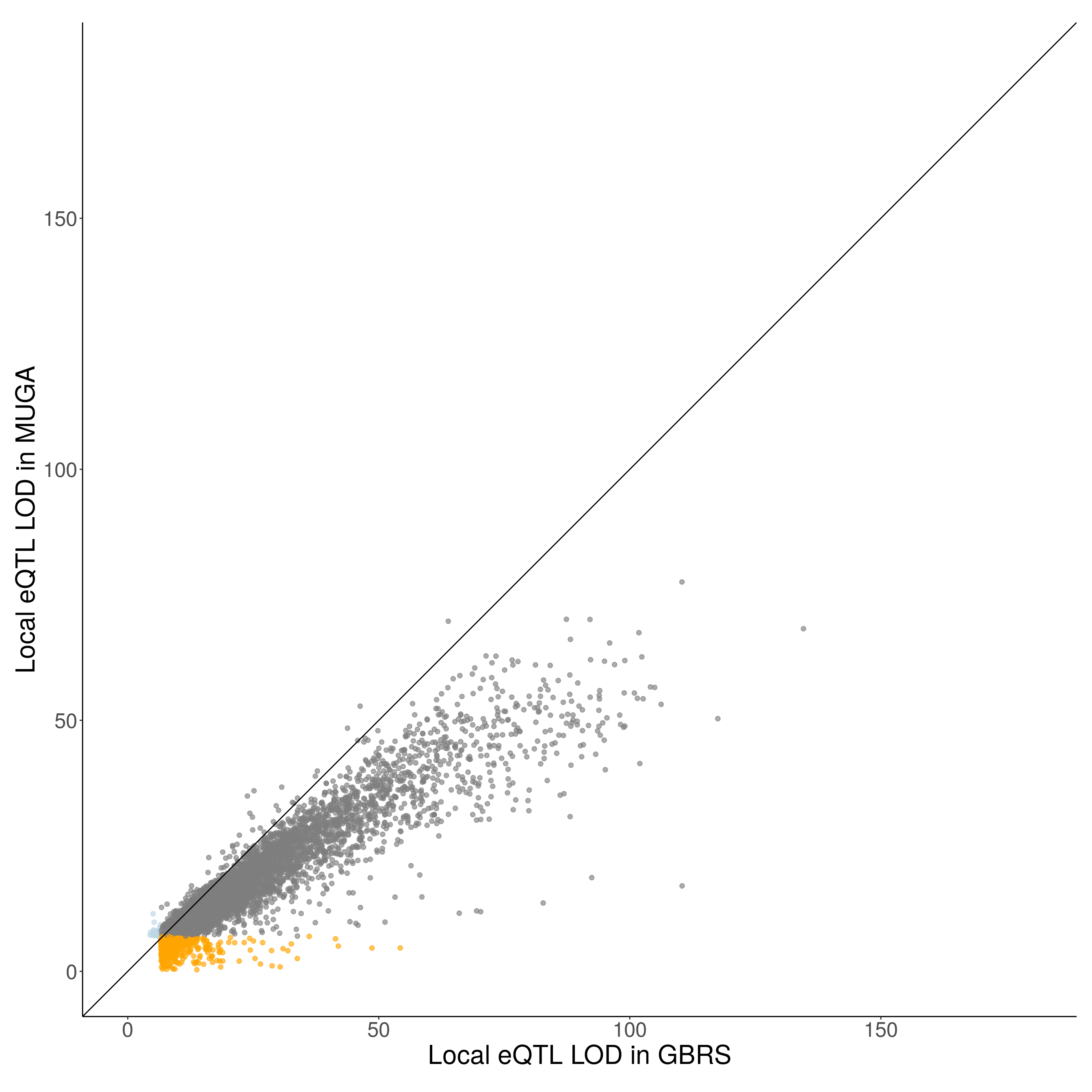



$MEGAMUGA_VS_GBRS
$MEGAMUGA_VS_GBRS$info
[1] "x:GBRS VS y:MEGAMUGA"

$MEGAMUGA_VS_GBRS$z

Both    x    y 
3940 1800   37 

$MEGAMUGA_VS_GBRS$down_up

Down   Up 
5257  520 

$MEGAMUGA_VS_GBRS$d1_mean
# A tibble: 2 x 4
  down_up mean_lodx mean_lody  diff
  <chr>       <dbl>     <dbl> <dbl>
1 Down         17.0      12.6  4.48
2 Up           10.7      11.9 -1.16

$MEGAMUGA_VS_GBRS$slope
(Intercept)    cislod.x 
  1.8474962   0.6468457 

$MEGAMUGA_VS_GBRS$plot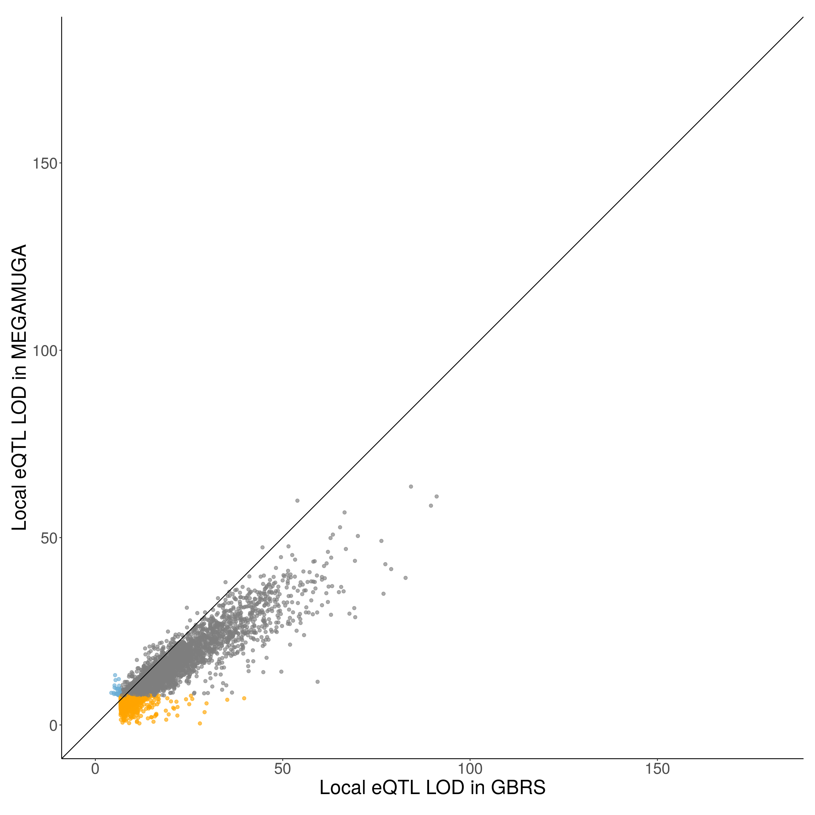



$GIGAMUGA_VS_GBRS
$GIGAMUGA_VS_GBRS$info
[1] "x:GBRS VS y:GIGAMUGA"

$GIGAMUGA_VS_GBRS$z

Both    x    y 
8456 1970  112 

$GIGAMUGA_VS_GBRS$down_up

Down   Up 
9682  856 

$GIGAMUGA_VS_GBRS$d1_mean
# A tibble: 2 x 4
  down_up mean_lodx mean_lody  diff
  <chr>       <dbl>     <dbl> <dbl>
1 Down         24.5      17.9  6.58
2 Up           13.8      15.8 -1.95

$GIGAMUGA_VS_GBRS$slope
(Intercept)    cislod.x 
  2.4850312   0.6458037 

$GIGAMUGA_VS_GBRS$plot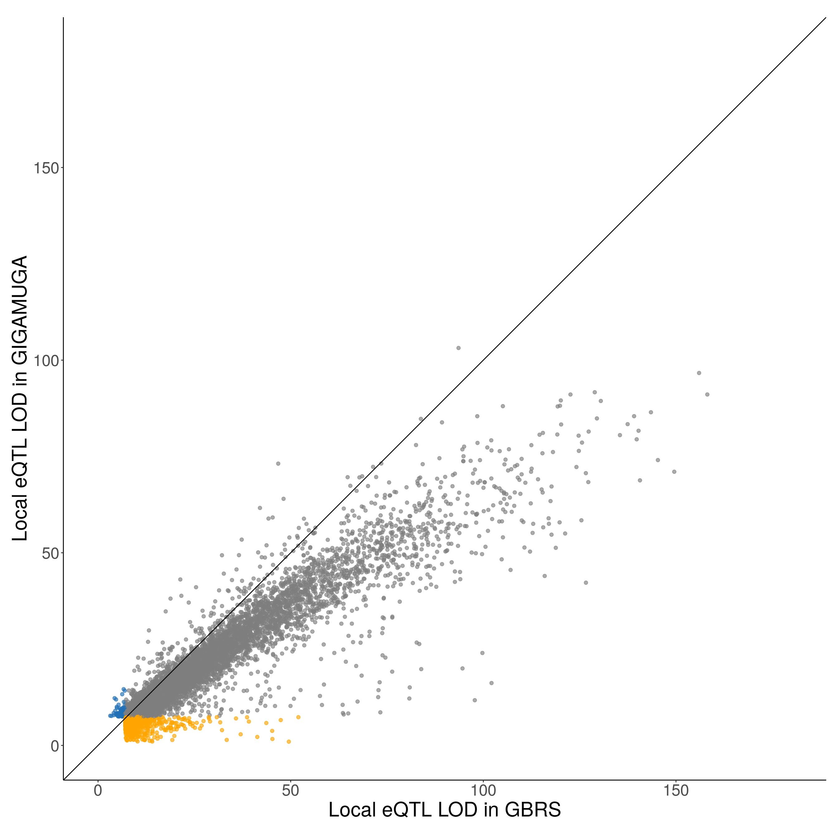

#table
df1 <- results_sum(results1)
df1 %>%
  kbl(caption = "Summary on beforefixedarray_vs_GBRS", digits = 3, align = "l") %>%
  kable_styling()

Summary on beforefixedarray_vs_GBRS
Infor	Var1	Freq	Down_Up	Freq	mean_lodx	mean_lody	diff	Intercept	Slope
x:GBRS VS y:MUGA	Both	5844						2.260	0.613
	x	1567	Down	6998	21.457	15.210	6.247
	y	52	Up	465	10.950	12.037	-1.087
x:GBRS VS y:MEGAMUGA	Both	3940						1.847	0.647
	x	1800	Down	5257	17.043	12.564	4.479
	y	37	Up	520	10.735	11.899	-1.163
x:GBRS VS y:GIGAMUGA	Both	8456						2.485	0.646
	x	1970	Down	9682	24.512	17.929	6.583
	y	112	Up	856	13.845	15.792	-1.947

Figure6_fixedarray_vs_GBRS

#parameters
xi      <- c("gbrs275", "gbrs184", "gbrs358")
yi      <- c("fixed.muga275", "fixed.megamuga184",  "fixed.gigamuga358")
x         <- cis.eqtl.total[xi]
name_xi   <- list("GBRS","GBRS", "GBRS")
cutoff_x  <- cutoff[xi]
y         <- cis.eqtl.total[yi]
name_yi   <- list("FIXED.MUGA","FIXED.MEGAMUGA", "FIXED.GIGAMUGA")
cutoff_y  <- cutoff[yi]
color     <- list("#bdd7e7", "#6baed6", "#2171b5")

#args
args <- list(x        = x,
             name_xi  = name_xi,
             cutoff_x = cutoff_x,
             y        = y,
             name_yi  = name_yi,
             cutoff_y = cutoff_y,
             color    = color)

results2 <- args %>% future_pmap(comparison_cis)
names(results2) <- paste0(name_yi, "_VS_", name_xi)
print(results2)

$FIXED.MUGA_VS_GBRS
$FIXED.MUGA_VS_GBRS$info
[1] "x:GBRS VS y:FIXED.MUGA"

$FIXED.MUGA_VS_GBRS$z

Both    x    y 
6754  657  161 

$FIXED.MUGA_VS_GBRS$down_up

Down   Up 
5910 1662 

$FIXED.MUGA_VS_GBRS$d1_mean
# A tibble: 2 x 4
  down_up mean_lodx mean_lody  diff
  <chr>       <dbl>     <dbl> <dbl>
1 Down         22.2      19.1  3.03
2 Up           15.0      16.2 -1.12

$FIXED.MUGA_VS_GBRS$slope
(Intercept)    cislod.x 
  1.0003732   0.8486424 

$FIXED.MUGA_VS_GBRS$plot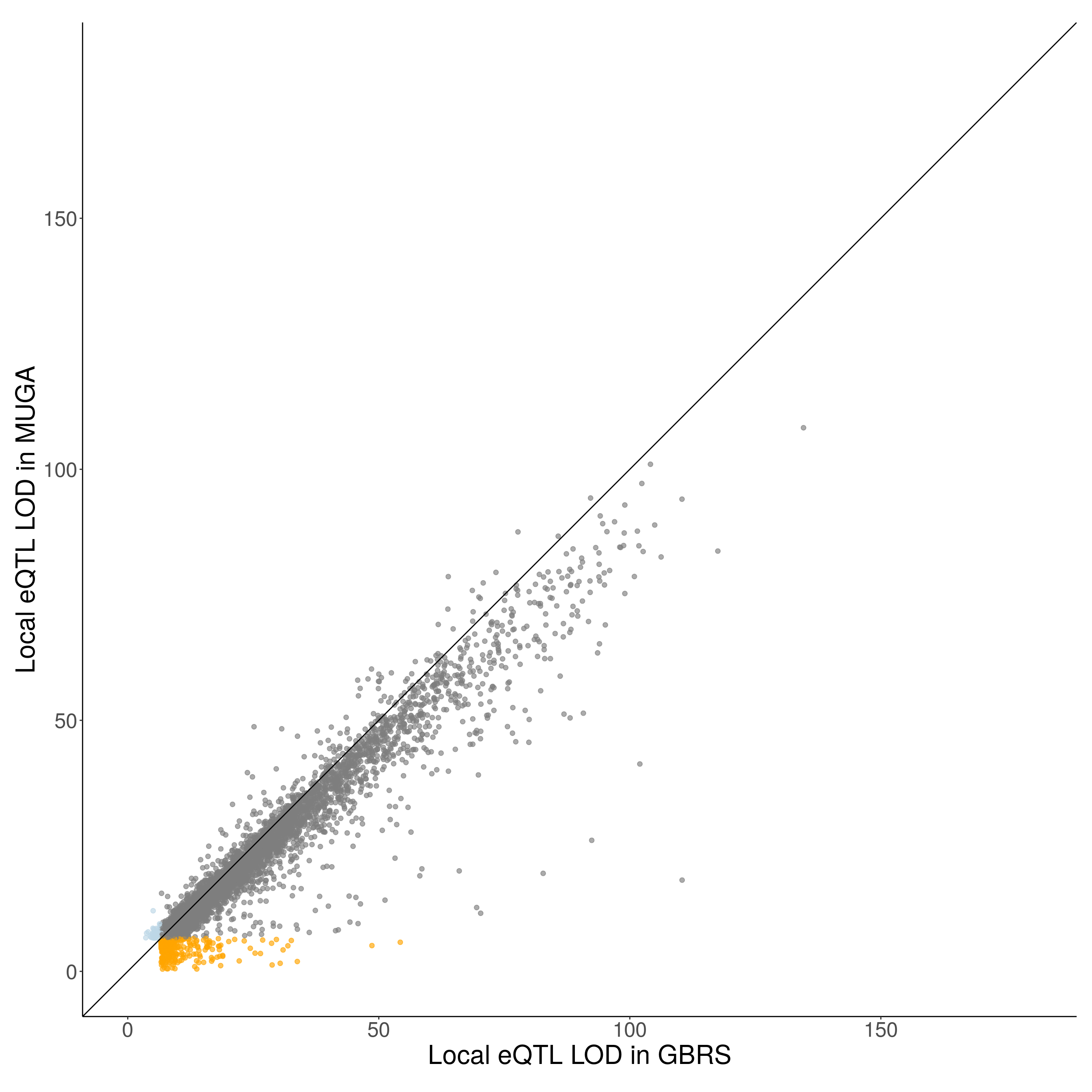



$FIXED.MEGAMUGA_VS_GBRS
$FIXED.MEGAMUGA_VS_GBRS$info
[1] "x:GBRS VS y:FIXED.MEGAMUGA"

$FIXED.MEGAMUGA_VS_GBRS$z

Both    x    y 
5270  470  171 

$FIXED.MEGAMUGA_VS_GBRS$down_up

Down   Up 
3673 2238 

$FIXED.MEGAMUGA_VS_GBRS$d1_mean
# A tibble: 2 x 4
  down_up mean_lodx mean_lody  diff
  <chr>       <dbl>     <dbl> <dbl>
1 Down         17.3      15.7  1.66
2 Up           14.5      15.7 -1.22

$FIXED.MEGAMUGA_VS_GBRS$slope
(Intercept)    cislod.x 
  0.5350914   0.9322379 

$FIXED.MEGAMUGA_VS_GBRS$plot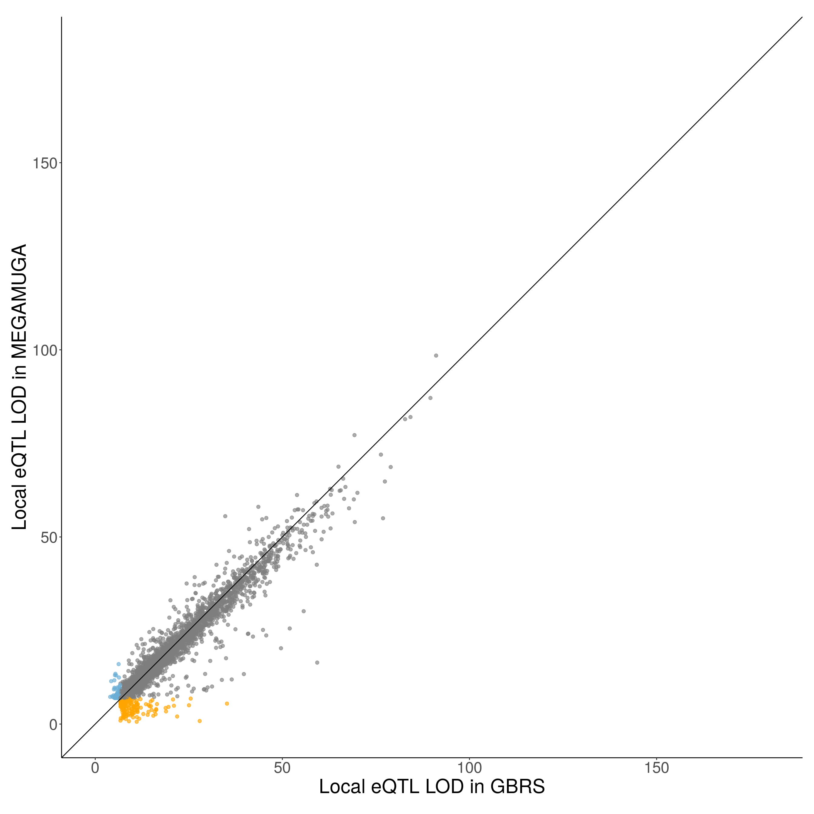



$FIXED.GIGAMUGA_VS_GBRS
$FIXED.GIGAMUGA_VS_GBRS$info
[1] "x:GBRS VS y:FIXED.GIGAMUGA"

$FIXED.GIGAMUGA_VS_GBRS$z

Both    x    y 
9671  755  305 

$FIXED.GIGAMUGA_VS_GBRS$down_up

Down   Up 
8051 2680 

$FIXED.GIGAMUGA_VS_GBRS$d1_mean
# A tibble: 2 x 4
  down_up mean_lodx mean_lody  diff
  <chr>       <dbl>     <dbl> <dbl>
1 Down         25.4      21.8  3.54
2 Up           17.3      19.4 -2.17

$FIXED.GIGAMUGA_VS_GBRS$slope
(Intercept)    cislod.x 
  1.5120940   0.8445103 

$FIXED.GIGAMUGA_VS_GBRS$plot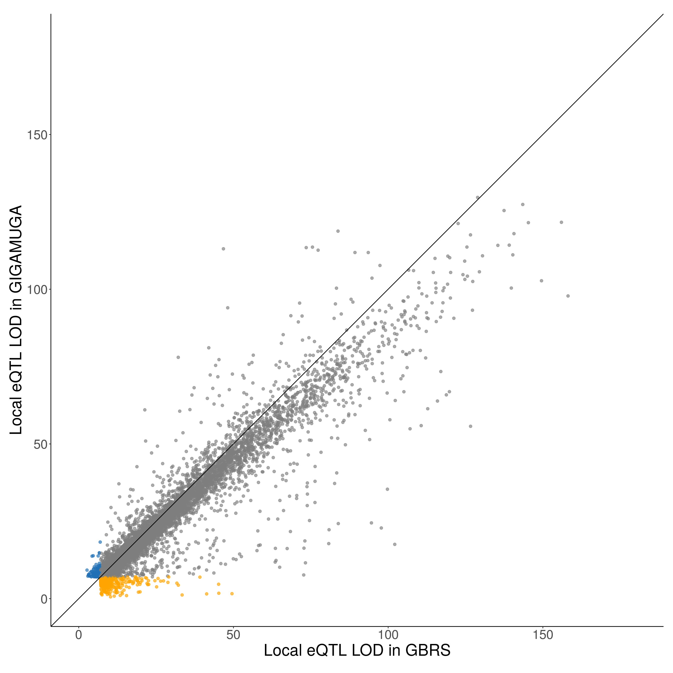

#table
df2 <- results_sum(results2)
df2 %>%
  kbl(caption = "Summary on fixedarray_vs_GBRS", digits = 3, align = "l") %>%
  kable_styling()

Summary on fixedarray_vs_GBRS
Infor	Var1	Freq	Down_Up	Freq	mean_lodx	mean_lody	diff	Intercept	Slope
x:GBRS VS y:FIXED.MUGA	Both	6754						1.000	0.849
	x	657	Down	5910	22.152	19.124	3.028
	y	161	Up	1662	15.043	16.167	-1.124
x:GBRS VS y:FIXED.MEGAMUGA	Both	5270						0.535	0.932
	x	470	Down	3673	17.309	15.653	1.655
	y	171	Up	2238	14.492	15.716	-1.223
x:GBRS VS y:FIXED.GIGAMUGA	Both	9671						1.512	0.845
	x	755	Down	8051	25.353	21.812	3.541
	y	305	Up	2680	17.267	19.432	-2.166

Figure6_combine_vs_GBRS

#parameters
xi      <- c("combine.fixed.gbrs275", "combine.fixed.gbrs184",      "combine.fixed.gbrs358")
yi      <- c("combine.fixed.muga275", "combine.fixed.megamuga184",  "combine.fixed.gigamuga358")
x         <- cis.eqtl.total[xi]
name_xi   <- list("GBRS","GBRS", "GBRS")
cutoff_x  <- cutoff[xi]
y         <- cis.eqtl.total[yi]
name_yi   <- list("COMBINE.MUGA","COMBINE.MEGAMUGA", "COMBINE.GIGAMUGA")
cutoff_y  <- cutoff[yi]
color     <- list("#bdd7e7", "#6baed6", "#2171b5")

#args
args <- list(x        = x,
             name_xi  = name_xi,
             cutoff_x = cutoff_x,
             y        = y,
             name_yi  = name_yi,
             cutoff_y = cutoff_y,
             color    = color)

results3 <- args %>% future_pmap(comparison_cis)
names(results3) <- paste0(name_yi, "_VS_", name_xi)
print(results3)

$COMBINE.MUGA_VS_GBRS
$COMBINE.MUGA_VS_GBRS$info
[1] "x:GBRS VS y:COMBINE.MUGA"

$COMBINE.MUGA_VS_GBRS$z

Both    x    y 
6647  792   50 

$COMBINE.MUGA_VS_GBRS$down_up

Down   Up 
5499 1990 

$COMBINE.MUGA_VS_GBRS$d1_mean
# A tibble: 2 x 4
  down_up mean_lodx mean_lody   diff
  <chr>       <dbl>     <dbl>  <dbl>
1 Down         21.5      19.3  2.26 
2 Up           16.4      17.2 -0.841

$COMBINE.MUGA_VS_GBRS$slope
(Intercept)    cislod.x 
  0.4983944   0.9042165 

$COMBINE.MUGA_VS_GBRS$plot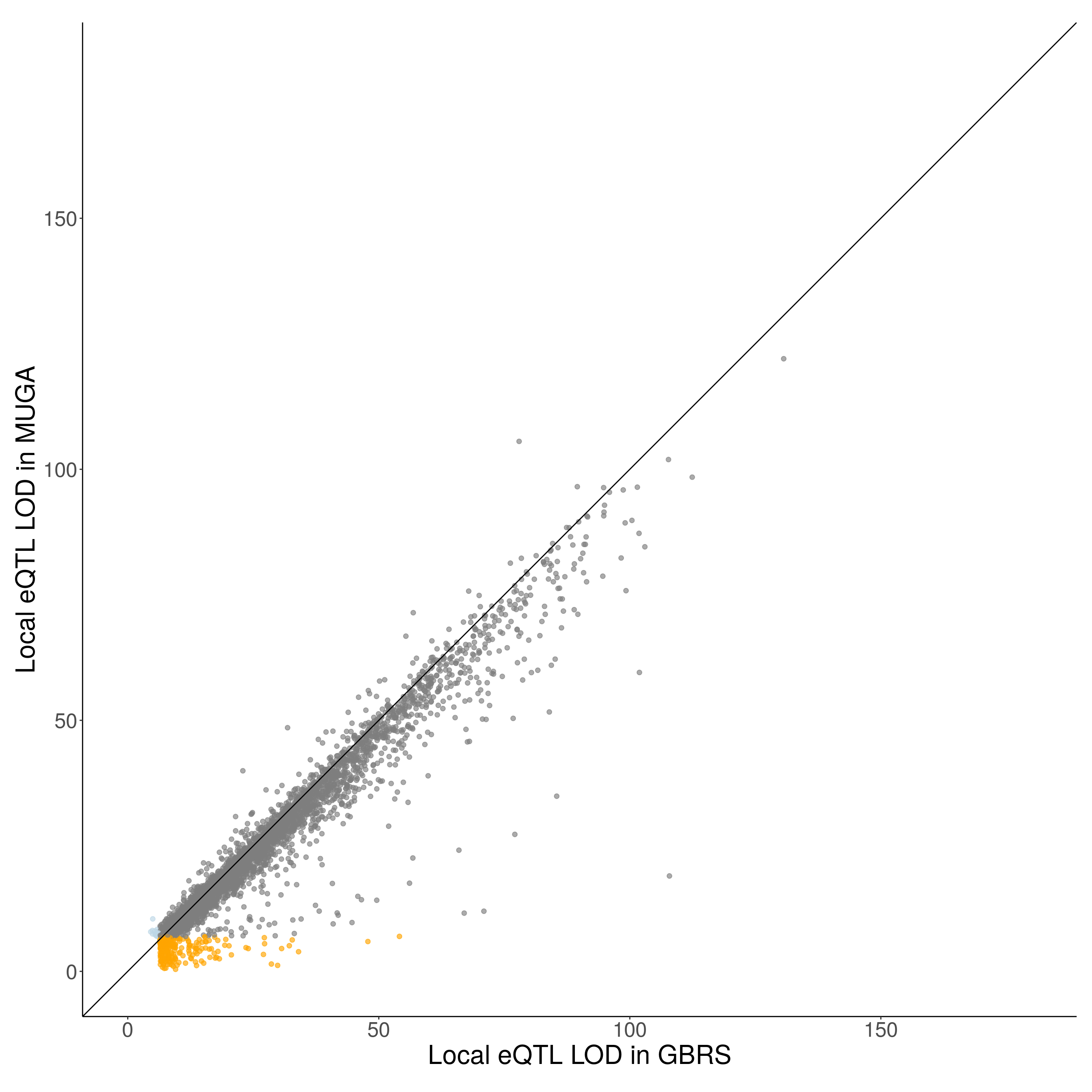



$COMBINE.MEGAMUGA_VS_GBRS
$COMBINE.MEGAMUGA_VS_GBRS$info
[1] "x:GBRS VS y:COMBINE.MEGAMUGA"

$COMBINE.MEGAMUGA_VS_GBRS$z

Both    x    y 
4865  916   15 

$COMBINE.MEGAMUGA_VS_GBRS$down_up

Down   Up 
3871 1925 

$COMBINE.MEGAMUGA_VS_GBRS$d1_mean
# A tibble: 2 x 4
  down_up mean_lodx mean_lody   diff
  <chr>       <dbl>     <dbl>  <dbl>
1 Down         17.0      15.5  1.51 
2 Up           14.8      15.6 -0.766

$COMBINE.MEGAMUGA_VS_GBRS$slope
(Intercept)    cislod.x 
  0.2996919   0.9351825 

$COMBINE.MEGAMUGA_VS_GBRS$plot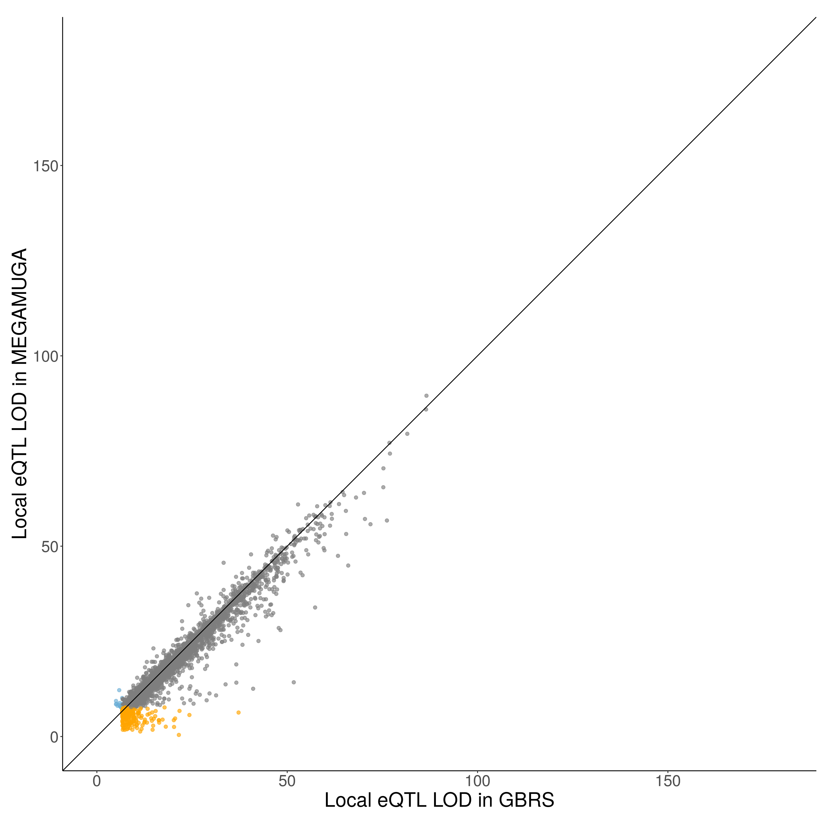



$COMBINE.GIGAMUGA_VS_GBRS
$COMBINE.GIGAMUGA_VS_GBRS$info
[1] "x:GBRS VS y:COMBINE.GIGAMUGA"

$COMBINE.GIGAMUGA_VS_GBRS$z

Both    x    y 
9367  753  176 

$COMBINE.GIGAMUGA_VS_GBRS$down_up

Down   Up 
7068 3228 

$COMBINE.GIGAMUGA_VS_GBRS$d1_mean
# A tibble: 2 x 4
  down_up mean_lodx mean_lody  diff
  <chr>       <dbl>     <dbl> <dbl>
1 Down         24.6      21.7  2.90
2 Up           19.7      21.3 -1.52

$COMBINE.GIGAMUGA_VS_GBRS$slope
(Intercept)    cislod.x 
  0.8215733   0.8984933 

$COMBINE.GIGAMUGA_VS_GBRS$plot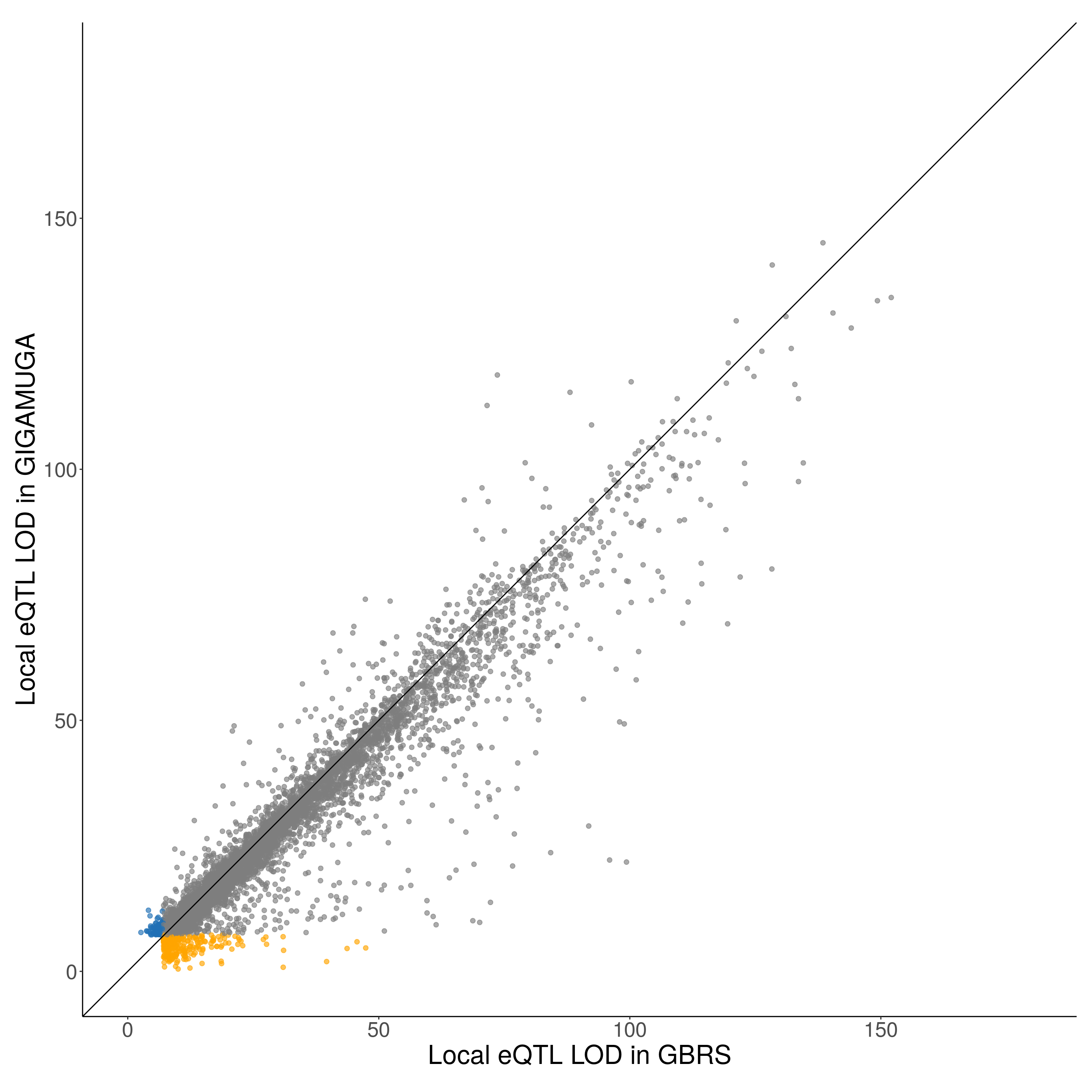

#table
df3 <- results_sum(results3)
df3 %>%
  kbl(caption = "Summary on combine_vs_GBRS", digits = 3, align = "l") %>%
  kable_styling()

Summary on combine_vs_GBRS
Infor	Var1	Freq	Down_Up	Freq	mean_lodx	mean_lody	diff	Intercept	Slope
x:GBRS VS y:COMBINE.MUGA	Both	6647						0.498	0.904
	x	792	Down	5499	21.533	19.276	2.257
	y	50	Up	1990	16.404	17.245	-0.841
x:GBRS VS y:COMBINE.MEGAMUGA	Both	4865						0.300	0.935
	x	916	Down	3871	17.021	15.508	1.513
	y	15	Up	1925	14.826	15.591	-0.766
x:GBRS VS y:COMBINE.GIGAMUGA	Both	9367						0.822	0.898
	x	753	Down	7068	24.556	21.653	2.903
	y	176	Up	3228	19.735	21.251	-1.516

Figure6_beforefixedarray_vs_combined

#parameters
xi      <- c("combine.fixed.muga275", "combine.fixed.megamuga184",  "combine.fixed.gigamuga358")
yi      <- c("muga275",               "megamuga184",                "gigamuga358")
x         <- cis.eqtl.total[xi]
name_xi   <- list("COMBINE","COMBINE", "COMBINE")
cutoff_x  <- cutoff[xi]
y         <- cis.eqtl.total[yi]
name_yi   <- list("MUGA","MEGAMUGA", "GIGAMUGA")
cutoff_y  <- cutoff[yi]
color     <- list("#bdd7e7", "#6baed6", "#2171b5")

#args
args <- list(x        = x,
             name_xi  = name_xi,
             cutoff_x = cutoff_x,
             y        = y,
             name_yi  = name_yi,
             cutoff_y = cutoff_y,
             color    = color)

results4 <- args %>% future_pmap(comparison_cis)
names(results4) <- paste0(name_yi, "_VS_", name_xi)
print(results4)

$MUGA_VS_COMBINE
$MUGA_VS_COMBINE$info
[1] "x:COMBINE VS y:MUGA"

$MUGA_VS_COMBINE$z

Both    x    y 
5776  916  117 

$MUGA_VS_COMBINE$down_up

Down   Up 
6002  807 

$MUGA_VS_COMBINE$d1_mean
# A tibble: 2 x 4
  down_up mean_lodx mean_lody  diff
  <chr>       <dbl>     <dbl> <dbl>
1 Down         21.1      16.3  4.74
2 Up           12.4      13.5 -1.11

$MUGA_VS_COMBINE$slope
(Intercept)    cislod.x 
  2.0605021   0.6951661 

$MUGA_VS_COMBINE$plot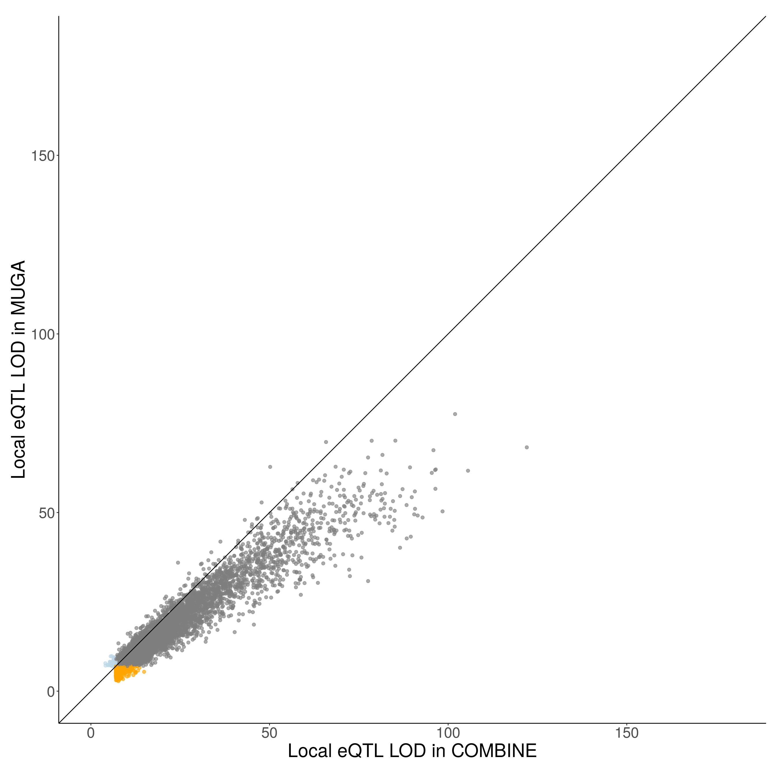



$MEGAMUGA_VS_COMBINE
$MEGAMUGA_VS_COMBINE$info
[1] "x:COMBINE VS y:MEGAMUGA"

$MEGAMUGA_VS_COMBINE$z

Both    x    y 
3888  990   86 

$MEGAMUGA_VS_COMBINE$down_up

Down   Up 
4358  606 

$MEGAMUGA_VS_COMBINE$d1_mean
# A tibble: 2 x 4
  down_up mean_lodx mean_lody  diff
  <chr>       <dbl>     <dbl> <dbl>
1 Down         17.7      13.7  4.05
2 Up           12.0      13.2 -1.24

$MEGAMUGA_VS_COMBINE$slope
(Intercept)    cislod.x 
  1.9262312   0.6872211 

$MEGAMUGA_VS_COMBINE$plot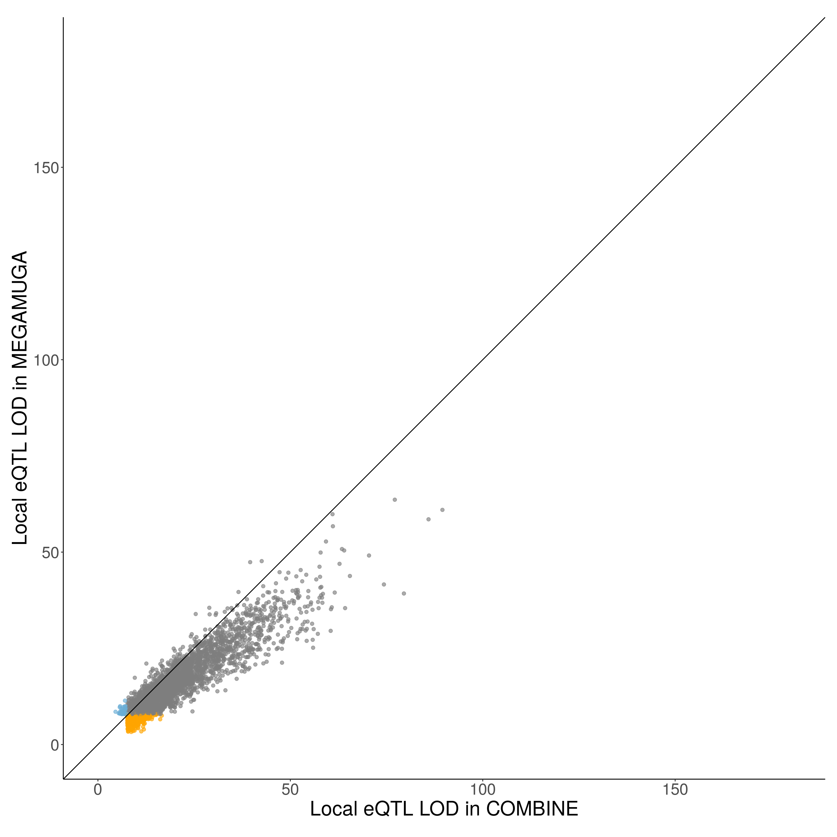



$GIGAMUGA_VS_COMBINE
$GIGAMUGA_VS_COMBINE$info
[1] "x:COMBINE VS y:GIGAMUGA"

$GIGAMUGA_VS_COMBINE$z

Both    x    y 
8374 1164  192 

$GIGAMUGA_VS_COMBINE$down_up

Down   Up 
8095 1635 

$GIGAMUGA_VS_COMBINE$d1_mean
# A tibble: 2 x 4
  down_up mean_lodx mean_lody  diff
  <chr>       <dbl>     <dbl> <dbl>
1 Down         24.0      19.3  4.68
2 Up           14.8      16.3 -1.51

$GIGAMUGA_VS_COMBINE$slope
(Intercept)    cislod.x 
  2.2557583   0.7369356 

$GIGAMUGA_VS_COMBINE$plot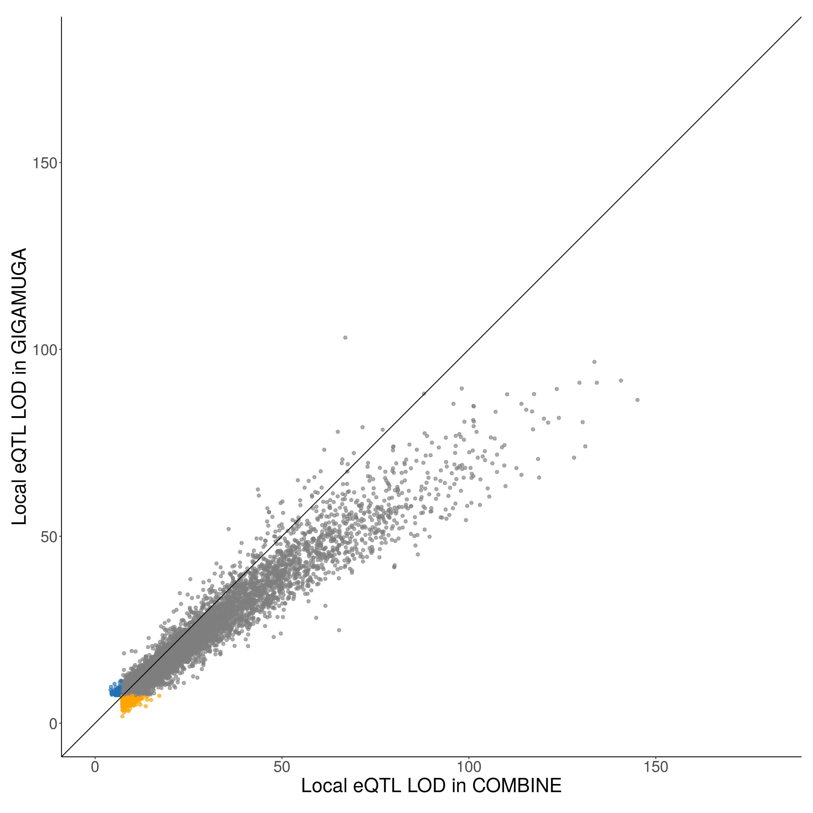

#table
df4 <- results_sum(results4)
df4 %>%
  kbl(caption = "Summary on beforefixedarray_vs_combined", digits = 3, align = "l") %>%
  kable_styling()

Summary on beforefixedarray_vs_combined
Infor	Var1	Freq	Down_Up	Freq	mean_lodx	mean_lody	diff	Intercept	Slope
x:COMBINE VS y:MUGA	Both	5776						2.061	0.695
	x	916	Down	6002	21.051	16.312	4.738
	y	117	Up	807	12.436	13.545	-1.109
x:COMBINE VS y:MEGAMUGA	Both	3888						1.926	0.687
	x	990	Down	4358	17.749	13.699	4.050
	y	86	Up	606	11.968	13.204	-1.236
x:COMBINE VS y:GIGAMUGA	Both	8374						2.256	0.737
	x	1164	Down	8095	23.974	19.290	4.684
	y	192	Up	1635	14.751	16.260	-1.510

Figure6_fixedarray_vs_combined

#parameters
xi      <- c("combine.fixed.muga275", "combine.fixed.megamuga184",  "combine.fixed.gigamuga358")
yi      <- c("fixed.muga275",               "fixed.megamuga184",                "fixed.gigamuga358")
x         <- cis.eqtl.total[xi]
name_xi   <- list("COMBINE","COMBINE", "COMBINE")
cutoff_x  <- cutoff[xi]
y         <- cis.eqtl.total[yi]
name_yi   <- list("FIXED.MUGA","FIXED.MEGAMUGA", "FIXED.GIGAMUGA")
cutoff_y  <- cutoff[yi]
color     <- list("#bdd7e7", "#6baed6", "#2171b5")

#args
args <- list(x        = x,
             name_xi  = name_xi,
             cutoff_x = cutoff_x,
             y        = y,
             name_yi  = name_yi,
             cutoff_y = cutoff_y,
             color    = color)

results5 <- args %>% future_pmap(comparison_cis)
names(results5) <- paste0(name_yi, "_VS_", name_xi)
print(results5)

$FIXED.MUGA_VS_COMBINE
$FIXED.MUGA_VS_COMBINE$info
[1] "x:COMBINE VS y:FIXED.MUGA"

$FIXED.MUGA_VS_COMBINE$z

Both    x    y 
6537  155  375 

$FIXED.MUGA_VS_COMBINE$down_up

Down   Up 
3604 3463 

$FIXED.MUGA_VS_COMBINE$d1_mean
# A tibble: 2 x 4
  down_up mean_lodx mean_lody  diff
  <chr>       <dbl>     <dbl> <dbl>
1 Down         21.1      19.6  1.50
2 Up           17.9      19.2 -1.32

$FIXED.MUGA_VS_COMBINE$slope
(Intercept)    cislod.x 
  0.5051509   0.9679814 

$FIXED.MUGA_VS_COMBINE$plot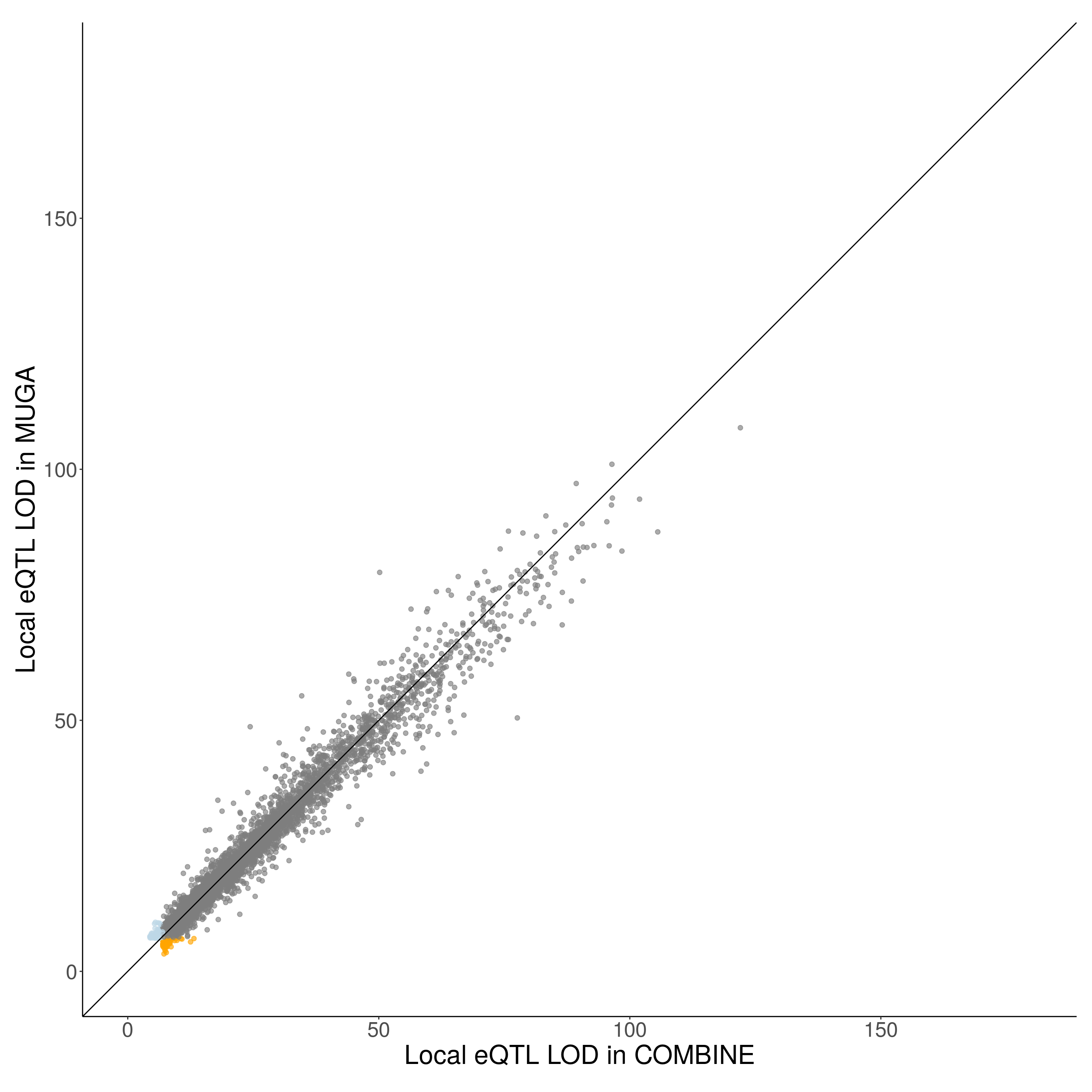



$FIXED.MEGAMUGA_VS_COMBINE
$FIXED.MEGAMUGA_VS_COMBINE$info
[1] "x:COMBINE VS y:FIXED.MEGAMUGA"

$FIXED.MEGAMUGA_VS_COMBINE$z

Both    x    y 
4846   32  592 

$FIXED.MEGAMUGA_VS_COMBINE$down_up

Down   Up 
2351 3119 

$FIXED.MEGAMUGA_VS_COMBINE$d1_mean
# A tibble: 2 x 4
  down_up mean_lodx mean_lody  diff
  <chr>       <dbl>     <dbl> <dbl>
1 Down         17.1      16.0  1.05
2 Up           15.4      16.8 -1.43

$FIXED.MEGAMUGA_VS_COMBINE$slope
(Intercept)    cislod.x 
  0.3879726   0.9983321 

$FIXED.MEGAMUGA_VS_COMBINE$plot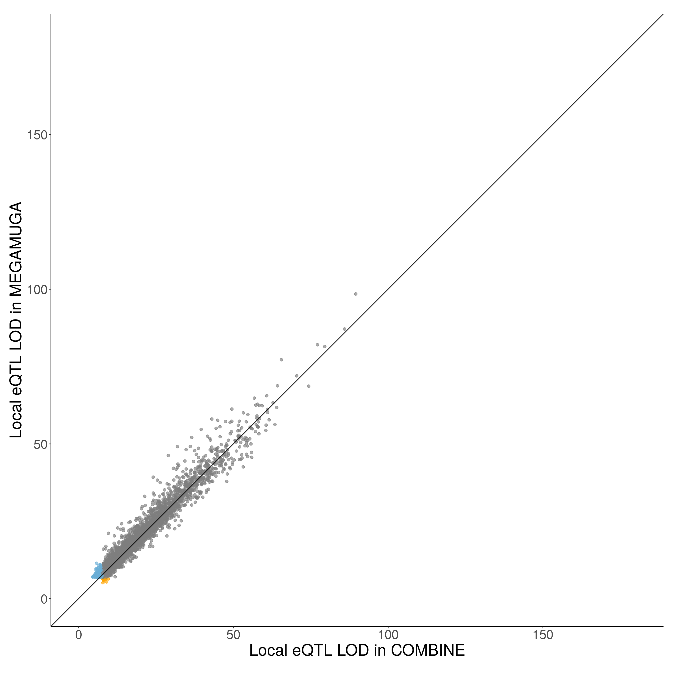



$FIXED.GIGAMUGA_VS_COMBINE
$FIXED.GIGAMUGA_VS_COMBINE$info
[1] "x:COMBINE VS y:FIXED.GIGAMUGA"

$FIXED.GIGAMUGA_VS_COMBINE$z

Both    x    y 
9339  199  634 

$FIXED.GIGAMUGA_VS_COMBINE$down_up

Down   Up 
4432 5740 

$FIXED.GIGAMUGA_VS_COMBINE$d1_mean
# A tibble: 2 x 4
  down_up mean_lodx mean_lody  diff
  <chr>       <dbl>     <dbl> <dbl>
1 Down         25.1      23.3  1.81
2 Up           19.1      21.1 -2.00

$FIXED.GIGAMUGA_VS_COMBINE$slope
(Intercept)    cislod.x 
   1.039462    0.967739 

$FIXED.GIGAMUGA_VS_COMBINE$plot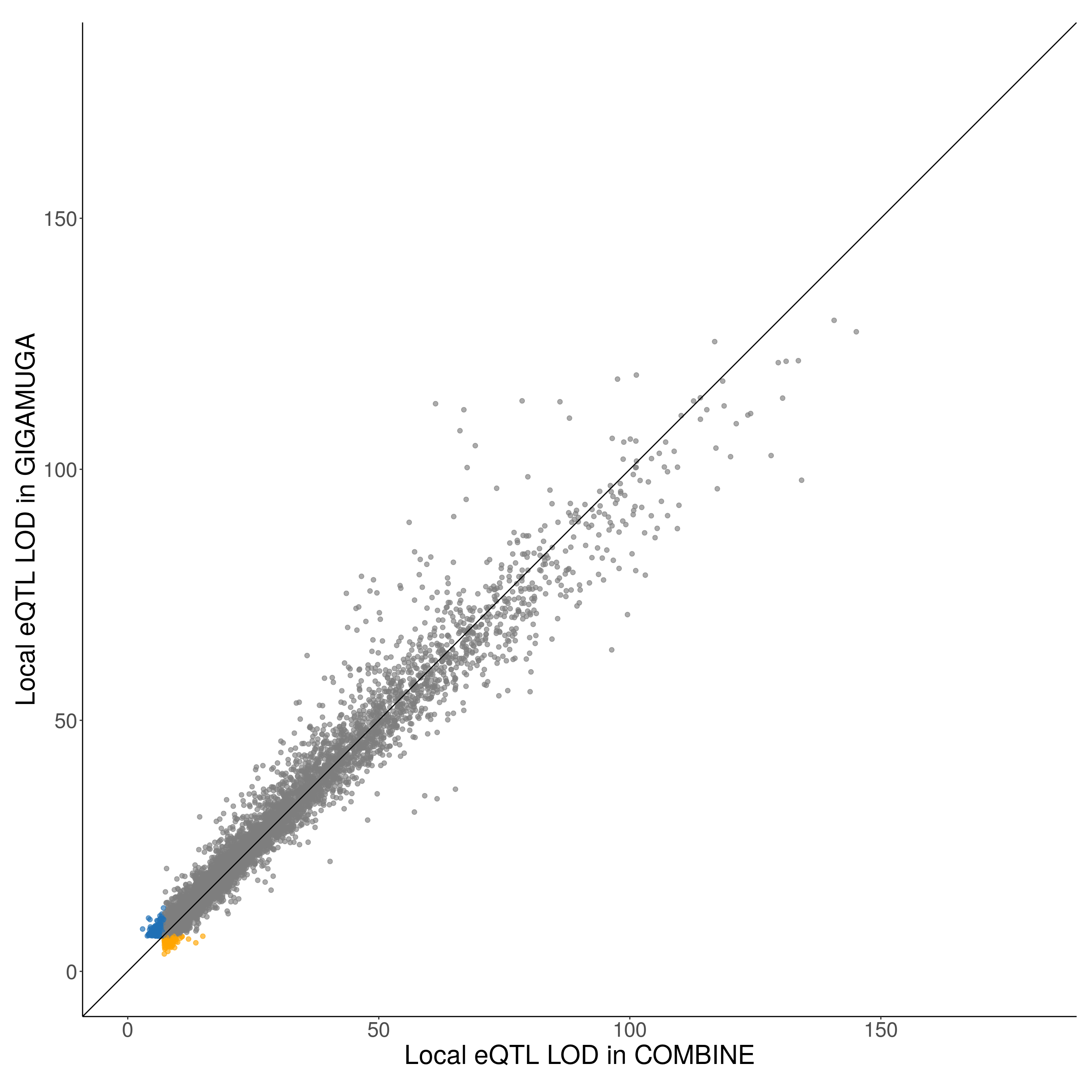

#table
df5 <- results_sum(results5)
df5 %>%
  kbl(caption = "Summary on fixedarray_vs_combined", digits = 3, align = "l") %>%
  kable_styling()

Summary on fixedarray_vs_combined
Infor	Var1	Freq	Down_Up	Freq	mean_lodx	mean_lody	diff	Intercept	Slope
x:COMBINE VS y:FIXED.MUGA	Both	6537						0.505	0.968
	x	155	Down	3604	21.107	19.607	1.500
	y	375	Up	3463	17.895	19.211	-1.316
x:COMBINE VS y:FIXED.MEGAMUGA	Both	4846						0.388	0.998
	x	32	Down	2351	17.070	16.019	1.051
	y	592	Up	3119	15.385	16.810	-1.425
x:COMBINE VS y:FIXED.GIGAMUGA	Both	9339						1.039	0.968
	x	199	Down	4432	25.088	23.279	1.809
	y	634	Up	5740	19.148	21.144	-1.996

sessionInfo()

R version 4.0.0 (2020-04-24)
Platform: x86_64-pc-linux-gnu (64-bit)
Running under: Ubuntu 18.04.4 LTS

Matrix products: default
BLAS/LAPACK: /usr/lib/x86_64-linux-gnu/libopenblasp-r0.2.20.so

locale:
 [1] LC_CTYPE=en_US.UTF-8       LC_NUMERIC=C              
 [3] LC_TIME=en_US.UTF-8        LC_COLLATE=en_US.UTF-8    
 [5] LC_MONETARY=en_US.UTF-8    LC_MESSAGES=C             
 [7] LC_PAPER=en_US.UTF-8       LC_NAME=C                 
 [9] LC_ADDRESS=C               LC_TELEPHONE=C            
[11] LC_MEASUREMENT=en_US.UTF-8 LC_IDENTIFICATION=C       

attached base packages:
[1] stats     graphics  grDevices utils     datasets  methods   base     

other attached packages:
 [1] kableExtra_1.3.1  furrr_0.2.1       future_1.20.1     ggpubr_0.4.0     
 [5] cowplot_1.1.0     viridis_0.5.1     viridisLite_0.3.0 MASS_7.3-51.6    
 [9] reshape2_1.4.4    plotly_4.9.2.1    gridExtra_2.3     qvalue_2.20.0    
[13] data.table_1.12.8 forcats_0.5.0     stringr_1.4.0     dplyr_1.0.0      
[17] purrr_0.3.4       readr_1.4.0       tidyr_1.1.0       tibble_3.0.1     
[21] tidyverse_1.3.0   ggplot2_3.3.2     workflowr_1.6.2  

loaded via a namespace (and not attached):
 [1] fs_1.4.1          lubridate_1.7.9   webshot_0.5.2     httr_1.4.1       
 [5] rprojroot_1.3-2   tools_4.0.0       backports_1.1.6   utf8_1.1.4       
 [9] R6_2.4.1          DBI_1.1.0         lazyeval_0.2.2    colorspace_1.4-1 
[13] withr_2.2.0       tidyselect_1.1.0  curl_4.3          compiler_4.0.0   
[17] git2r_0.27.1      cli_2.0.2         rvest_0.3.6       xml2_1.3.2       
[21] labeling_0.4.2    scales_1.1.1      digest_0.6.25     foreign_0.8-79   
[25] rmarkdown_2.5     rio_0.5.16        pkgconfig_2.0.3   htmltools_0.4.0  
[29] parallelly_1.21.0 highr_0.8         dbplyr_2.0.0      htmlwidgets_1.5.1
[33] rlang_0.4.6       readxl_1.3.1      rstudioapi_0.11   farver_2.0.3     
[37] generics_0.0.2    jsonlite_1.6.1    zip_2.1.1         car_3.0-10       
[41] magrittr_1.5      Rcpp_1.0.4.6      munsell_0.5.0     fansi_0.4.1      
[45] abind_1.4-5       lifecycle_0.2.0   stringi_1.4.6     whisker_0.4      
[49] yaml_2.2.1        carData_3.0-4     plyr_1.8.6        grid_4.0.0       
[53] parallel_4.0.0    listenv_0.8.0     promises_1.1.0    crayon_1.3.4     
[57] haven_2.3.1       splines_4.0.0     hms_0.5.3         knitr_1.28       
[61] pillar_1.4.4      ggsignif_0.6.0    codetools_0.2-16  reprex_0.3.0     
[65] glue_1.4.0        evaluate_0.14     modelr_0.1.8      vctrs_0.3.1      
[69] httpuv_1.5.4      cellranger_1.1.0  gtable_0.3.0      assertthat_0.2.1 
[73] xfun_0.13         openxlsx_4.2.3    broom_0.7.2       rstatix_0.6.0    
[77] later_1.0.0       globals_0.13.1    ellipsis_0.3.0