import torch
import torchvision
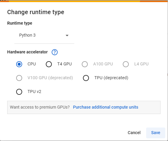
cifar_ds = torchvision.datasets.CIFAR100(root="/tmp", train=True, download=True)Files already downloaded and verifiedOn the top right corner of the page, click the drop-down arrow to the right of the Connect button and select Change runtime type.
Make sure Python 3 runtime is selected. For this part of the workshop CPU acceleration is enough.
Now we can connect to the runtime by clicking Connect. This will create a Virtual Machine (VM) with compute resources we can use for a limited amount of time.

Caution
In free Colab accounts these resources are not guaranteed and can be taken away without notice (preemptible machines).
Data stored in this runtime will be lost if not moved into other storage when the runtime is deleted.
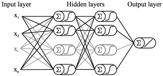
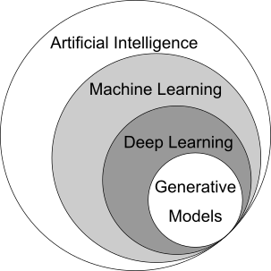
Sub-field of Artificial Intelligence that develops methods to address tasks that require human intelligence
Classification

what is this?
Detection
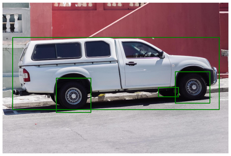
where is something?
Segmentation
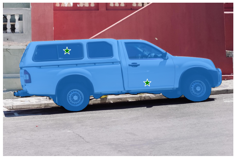
where specifically is something?
import torch
import torchvision
cifar_ds = torchvision.datasets.CIFAR100(root="/tmp", train=True, download=True)Files already downloaded and verifiedy = 19 (cattle)Models that construct knowledge in a hierarchical manner are considered deep models.
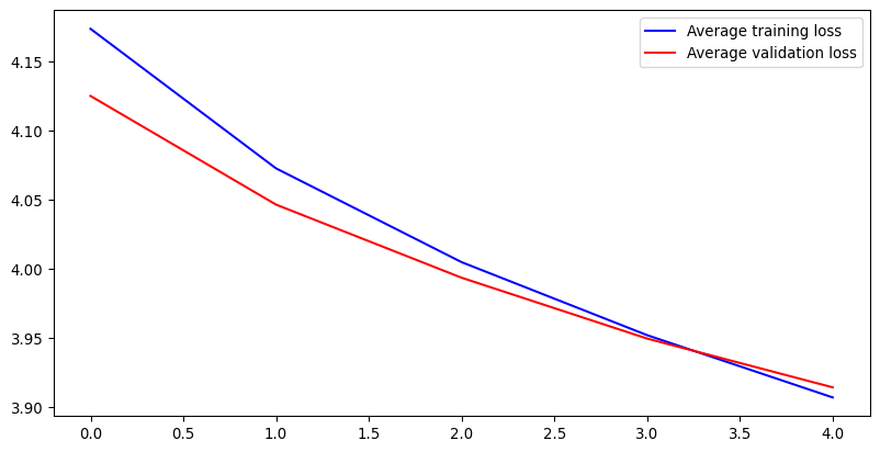
import matplotlib.pyplot as plt

plt.plot(train_loss, "b-", label="Training loss")
plt.plot([0, len(train_loss)], [train_loss_avg, train_loss_avg], "r:", label="Average training loss")
plt.plot([0, len(train_loss)], [val_loss_avg, val_loss_avg], "b:", label="Average validation loss")
plt.legend()
plt.show()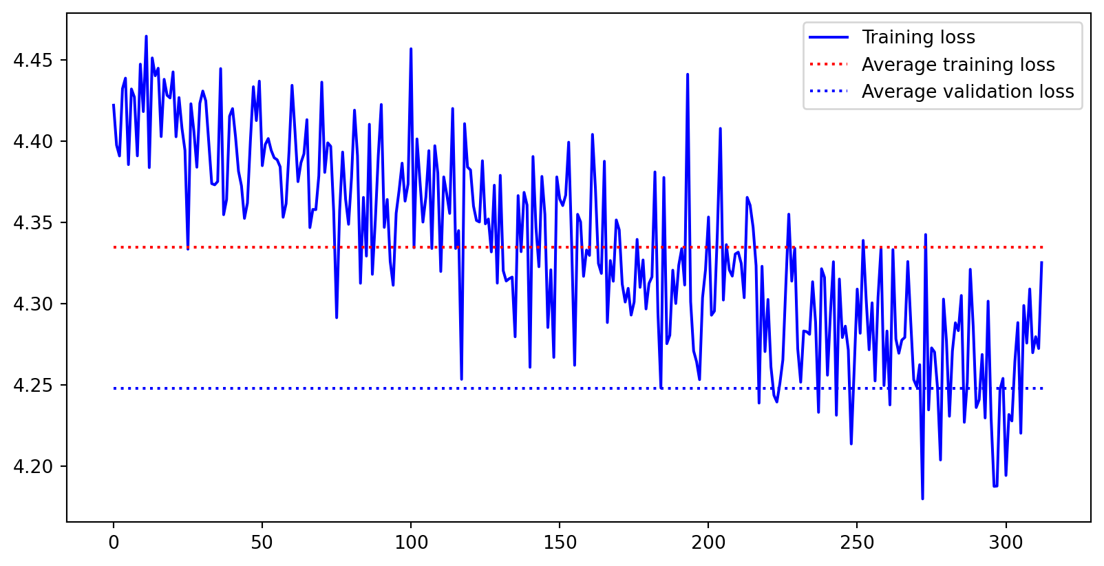
The most common operation in DL models for image processing are Convolution operations.
2D Convolution
The animation shows the convolution of a 7x7 pixels input image (bottom) with a 3x3 pixels kernel (moving window), that results in a 5x5 pixels output (top).
plt.rcParams['figure.figsize'] = [5, 5]

fig, ax = plt.subplots(1, 2)
ax[0].imshow(x[0].permute(1, 2, 0))
ax[1].imshow(fx.detach()[0, 0], cmap="gray")
plt.show()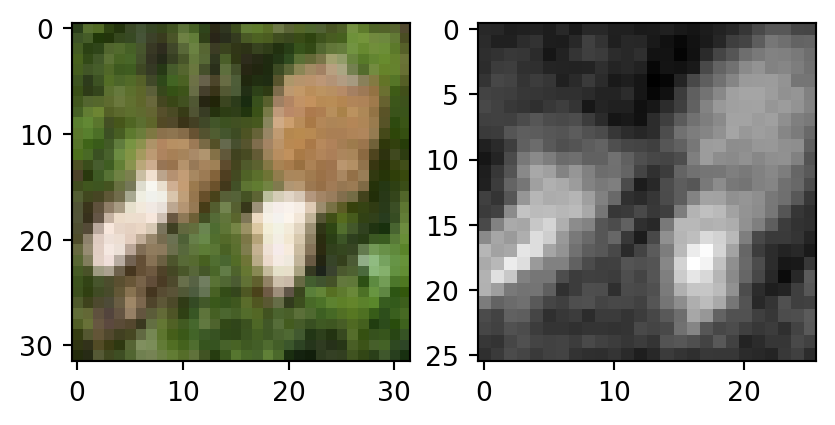
Important
By default, outputs from PyTorch modules are tracked for back-propagation.
To visualize it with matplotlib we have to .detach() the tensor first.
fx = conv_1(x)

fig, ax = plt.subplots(1, 2)
ax[0].imshow(x[0].permute(1, 2, 0))
ax[1].imshow(fx.detach()[0].permute(1, 2, 0))
plt.show()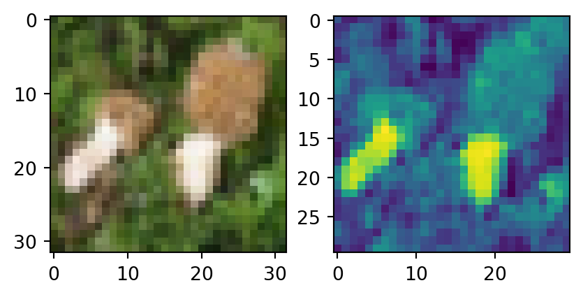
Experiment with different values and shapes of the kernel https://en.wikipedia.org/wiki/Kernel_(image_processing)
conv_1 = nn.Conv2d(in_channels=3, out_channels=1, kernel_size=3, padding=0, bias=False)

conv_1.weight.data[:] = torch.FloatTensor([
  [[[0, -1, 0], [-1, 5, -1], [0, -1, 0]],
   [[0, 0, 0], [0, 0, 0], [0, 0, 0]],
   [[0, 0, 0], [0, 0, 0], [0, 0, 0]]]
])

fx = conv_1(x)

fig, ax = plt.subplots(1, 2)
ax[0].imshow(x[0].permute(1, 2, 0))
ax[1].imshow(fx.detach()[0, 0], cmap="gray")
plt.show()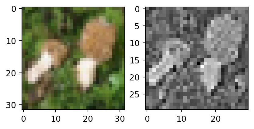
Experiment with different values and shapes of the kernel https://en.wikipedia.org/wiki/Kernel_(image_processing)
conv_1 = nn.Conv2d(in_channels=3, out_channels=1, kernel_size=3, padding=0, bias=False)

conv_1.weight.data[:] = torch.FloatTensor([
  [[[1, 0, -1], [1, 0, -1], [1, 0, -1]],
   [[1, 0, -1], [1, 0, -1], [1, 0, -1]],
   [[1, 0, -1], [1, 0, -1], [1, 0, -1]]]
])

fx = conv_1(x)

fig, ax = plt.subplots(1, 2)
ax[0].imshow(x[0].permute(1, 2, 0))
ax[1].imshow(fx.detach()[0, 0], cmap="gray")
plt.show()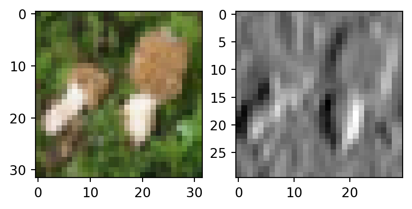
Experiment with different values and shapes of the kernel https://en.wikipedia.org/wiki/Kernel_(image_processing)
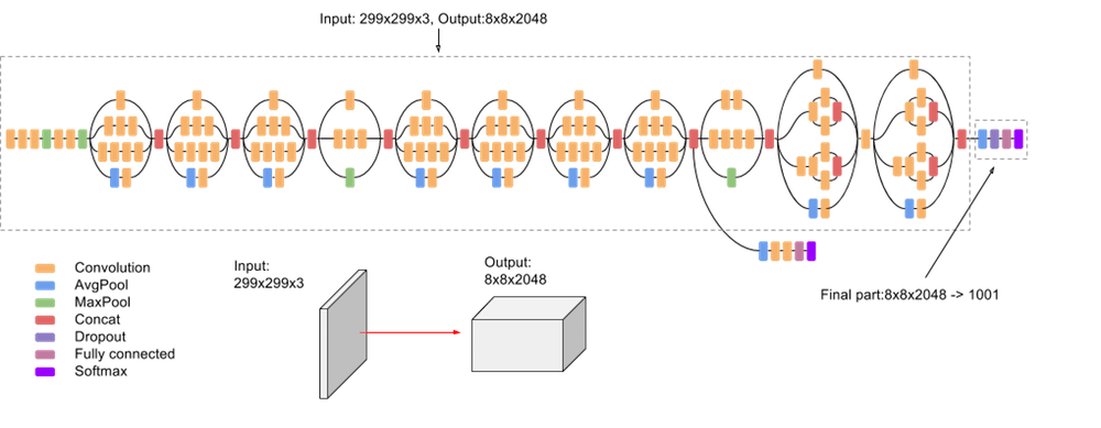
InceptionV3
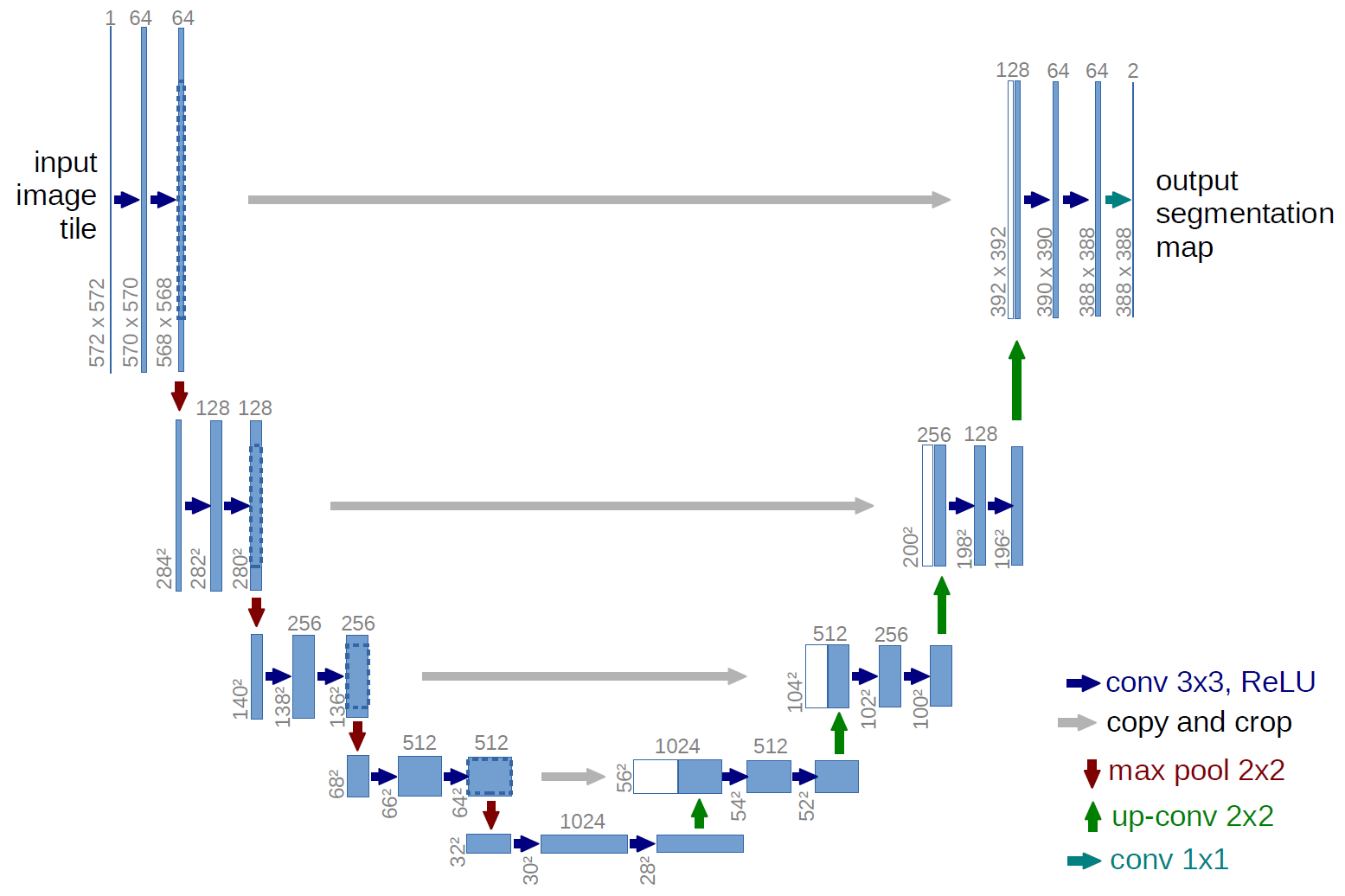
U-Net
 By Daniel Voigt Godoy - https://github.com/dvgodoy/dl-visuals/, CC BY 4.0, Link