Advanced Machine Learning with Python (Session 1 - Part 2)

Fernando Cervantes (fernando.cervantes@jax.org)

Materials

Open notebook in Colab View solutions

Convolutional Neural Network (CNN or ConvNet)

Convolution layers

The most common operation in DL models for image processing are Convolution operations.

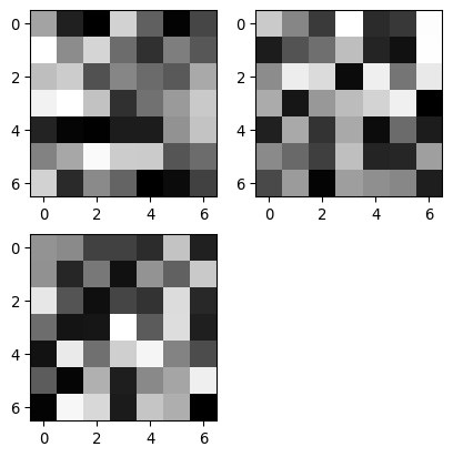
2D Convolution

The animation shows the convolution of a 7x7 pixels input image (bottom) with a 3x3 pixels kernel (moving window), that results in a 5x5 pixels output (top).

Exercise: Visualize the effect of the convolution operation

• Create a convolution layer with nn.Conv2D using 3 channels as input, and a single one for output.

import torch.nn as nn

conv_1 = nn.Conv2d(in_channels=3, out_channels=1, kernel_size=7, padding=0, bias=True)

x, _ = next(iter(cifar_train_dl))

fx = conv_1(x)

print("Input:", type(x), x.dtype, x.shape, x.min(), x.max())
print("Output:", type(fx), fx.dtype, fx.shape, fx.min(), fx.max())

Input: <class 'torch.Tensor'> torch.float32 torch.Size([128, 3, 32, 32]) tensor(0.) tensor(1.)
Output: <class 'torch.Tensor'> torch.float32 torch.Size([128, 1, 26, 26]) tensor(-0.8468, grad_fn=<MinBackward1>) tensor(0.1861, grad_fn=<MaxBackward1>)

Warning

The convolution layer is initialized with random values, so the results will vary.

Exercise: Visualize the effect of the convolution operation

• Create a convolution layer with nn.Conv2D using 3 channels as input, and a single one for output.

import matplotlib.pyplot as plt

plt.rcParams['figure.figsize'] = [5, 5]

fig, ax = plt.subplots(1, 2)
ax[0].imshow(x[0].permute(1, 2, 0))
ax[1].imshow(fx.detach()[0, 0], cmap="gray")
plt.show()

Important

By default, outputs from PyTorch modules are tracked for back-propagation.

To visualize it with matplotlib we have to .detach() the tensor first.

Exercise: Visualize the effect of the convolution operation

• Visualize the weights of the convolution layer.

conv_1.weight.shape

torch.Size([1, 3, 7, 7])

fig, ax = plt.subplots(2, 2)
ax[0, 0].imshow(conv_1.weight.detach()[0, 0], cmap="gray")
ax[0, 1].imshow(conv_1.weight.detach()[0, 1], cmap="gray")
ax[1, 0].imshow(conv_1.weight.detach()[0, 2], cmap="gray")
ax[1, 1].set_axis_off()
plt.show()

Exercise: Visualize the effect of the convolution operation

• Modify the weights of the convolution layer.

conv_1 = nn.Conv2d(in_channels=3, out_channels=1, kernel_size=3, padding=0, bias=False)

conv_1.weight.data[:] = torch.FloatTensor([
  [
    [
      [0, 0, 0],
      [0, 0, 0],
      [0, 0, 0],
    ],
    [
      [0, 0, 0],
      [0, 1, 0],
      [0, 0, 0],
    ],
    [
      [0, 0, 0],
      [0, 0, 0],
      [0, 0, 0],
    ],
  ]
])

Exercise: Visualize the effect of the convolution operation

• Visualize the effects after changing the values.

fx = conv_1(x)

fig, ax = plt.subplots(1, 2)
ax[0].imshow(x[0].permute(1, 2, 0))
ax[1].imshow(fx.detach()[0].permute(1, 2, 0))
plt.show()

Experiment with different values and shapes of the kernel https://en.wikipedia.org/wiki/Kernel_(image_processing)

Exercise: Visualize the effect of the convolution operation

• Modify the weights of the convolution layer.

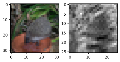
conv_1 = nn.Conv2d(in_channels=3, out_channels=1, kernel_size=3, padding=0, bias=False)

conv_1.weight.data[:] = torch.FloatTensor([
  [[[0, -1, 0], [-1, 5, -1], [0, -1, 0]],
   [[0, 0, 0], [0, 0, 0], [0, 0, 0]],
   [[0, 0, 0], [0, 0, 0], [0, 0, 0]]]
])

fx = conv_1(x)

fig, ax = plt.subplots(1, 2)
ax[0].imshow(x[0].permute(1, 2, 0))
ax[1].imshow(fx.detach()[0, 0], cmap="gray")
plt.show()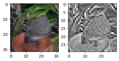

Experiment with different values and shapes of the kernel https://en.wikipedia.org/wiki/Kernel_(image_processing)

Exercise: Visualize the effect of the convolution operation

• Modify the weights of the convolution layer.

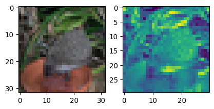
conv_1 = nn.Conv2d(in_channels=3, out_channels=1, kernel_size=3, padding=0, bias=False)

conv_1.weight.data[:] = torch.FloatTensor([
  [[[1, 0, -1], [1, 0, -1], [1, 0, -1]],
   [[1, 0, -1], [1, 0, -1], [1, 0, -1]],
   [[1, 0, -1], [1, 0, -1], [1, 0, -1]]]
])

fx = conv_1(x)

fig, ax = plt.subplots(1, 2)
ax[0].imshow(x[0].permute(1, 2, 0))
ax[1].imshow(fx.detach()[0, 0], cmap="gray")
plt.show()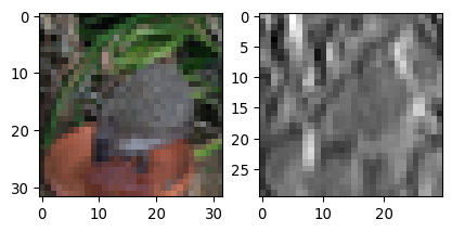

Experiment with different values and shapes of the kernel https://en.wikipedia.org/wiki/Kernel_(image_processing)

Examples of popular Deep Learning models in computer vision

• Residual Neural Networks

He, Kaiming et al. “Deep Residual Learning for Image Recognition.” 2016 IEEE Conference on Computer Vision and Pattern Recognition (CVPR) (2015): 770-778.

Examples of popular Deep Learning models in computer vision

• Inception (v3)

Szegedy, Christian et al. “Going deeper with convolutions.” 2015 IEEE Conference on Computer Vision and Pattern Recognition (CVPR) (2014): 1-9.

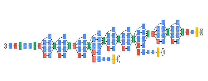
Examples of popular Deep Learning models in computer vision

• U-Net (cell segmentation)

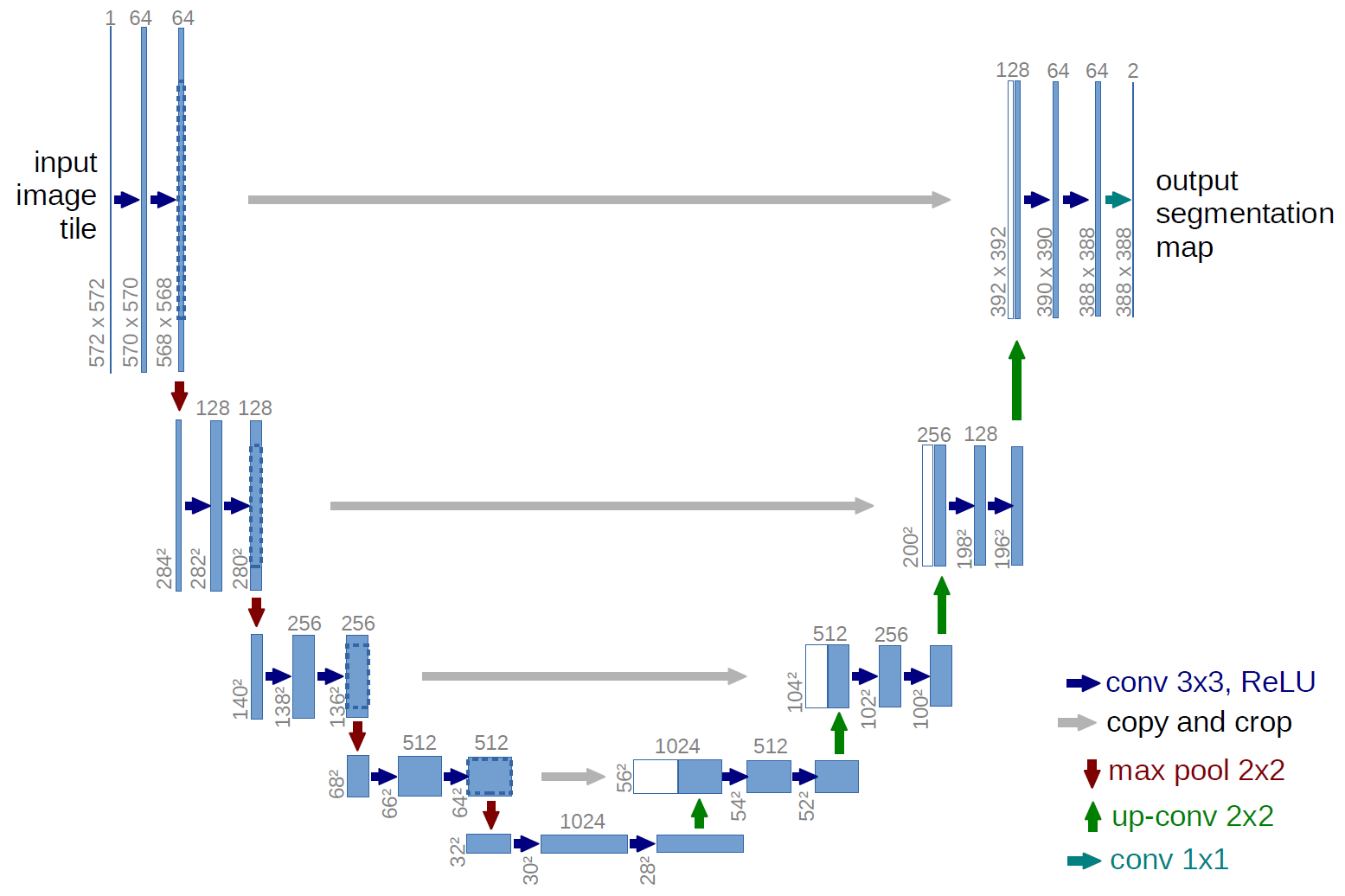
Ronneberger, Olaf et al. “U-Net: Convolutional Networks for Biomedical Image Segmentation.” ArXiv abs/1505.04597 (2015): n. pag.

Examples of popular Deep Learning models in computer vision

• Vision Transformer (classification and segmentation)

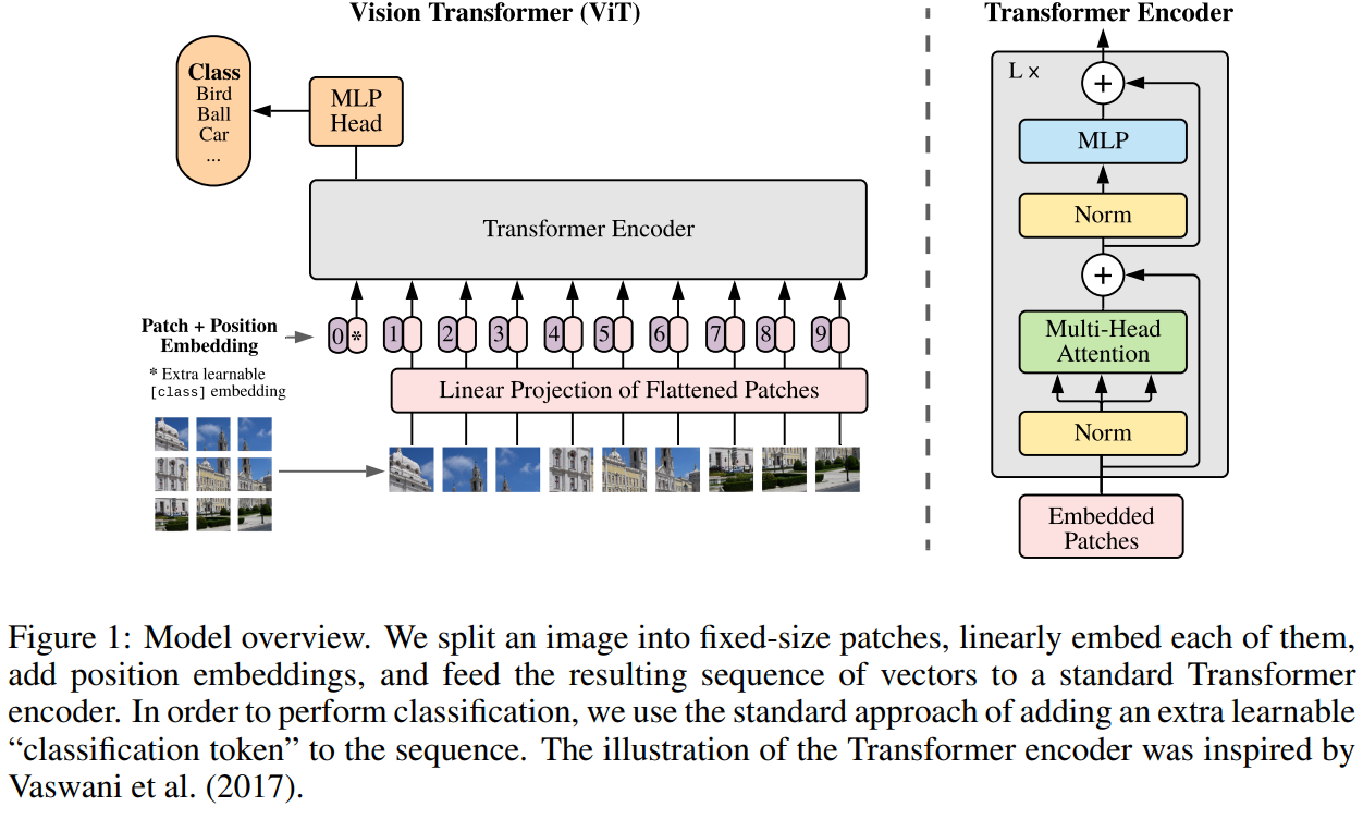
Dosovitskiy, Alexey et al. “An Image is Worth 16x16 Words: Transformers for Image Recognition at Scale.” ArXiv abs/2010.11929 (2020): n. pag.

• Segment Anything Model (SAM)
• Micro-SAM

Examples of popular Deep Learning models in computer vision

• LeNet-5 for handwritten digits classification (LeCun et al.)

LeCun, Yann et al. “Gradient-based learning applied to document recognition.” Proc. IEEE 86 (1998): 2278-2324.

By Daniel Voigt Godoy - https://github.com/dvgodoy/dl-visuals/, CC BY 4.0, Link

Exercise: Implement and train the LetNet-5 model with PyTorch

• Build the convolutional neural network using nn.Sequential, and the nn.ReLU() activation function.

lenet_clf = nn.Sequential(
    nn.Conv2d(in_channels=3, out_channels=6, kernel_size=5, bias=True),
    nn.ReLU(),
    nn.MaxPool2d(kernel_size=2),
    nn.Conv2d(in_channels=6, out_channels=16, kernel_size=5, bias=True),
    nn.ReLU(),
    nn.MaxPool2d(kernel_size=2),
    nn.Flatten(),
    nn.Linear(in_features=16*5*5, out_features=120, bias=True),
    nn.ReLU(),
    nn.Linear(in_features=120, out_features=84, bias=True),
    nn.ReLU(),
    nn.Linear(in_features=84, out_features=100, bias=True),
)

Note

Pooling layers are used to downsample feature maps to summarize information from large regions.

Exercise: Implement and train the LetNet-5 model with PyTorch

• Test our implementation.

y_hat = lenet_clf(x)

type(y_hat), y_hat.dtype, y_hat.shape, y_hat.min(), y_hat.max()

(torch.Tensor,
 torch.float32,
 torch.Size([128, 100]),
 tensor(-0.1309, grad_fn=<MinBackward1>),
 tensor(0.1939, grad_fn=<MaxBackward1>))

Exercise: Implement and train the LetNet-5 model with PyTorch

• Train the model to classify images from CIFAR-100.

import torch.optim as optim

num_epochs = 10
train_loss = []
val_loss = []

if torch.cuda.is_available():
  lenet_clf.cuda()

optimizer = optim.SGD(lenet_clf.parameters(), lr=0.01)
loss_fun = nn.CrossEntropyLoss()

for e in range(num_epochs):
  train_loss_avg = 0
  total_train_samples = 0

  lenet_clf.train()
  for x, y in cifar_train_dl:
    optimizer.zero_grad()

    if torch.cuda.is_available():
      x = x.cuda()
    
    y_hat = lenet_clf( x ).cpu()

    loss = loss_fun(y_hat, y)

    train_loss_avg += loss.item() * len(x)
    total_train_samples += len(x)

    loss.backward()

    optimizer.step()

  train_loss_avg /= total_train_samples
  train_loss.append(train_loss_avg)

  val_loss_avg = 0
  total_val_samples = 0

  lenet_clf.eval()
  with torch.no_grad():
    for x, y in cifar_val_dl:
      if torch.cuda.is_available():
        x = x.cuda()
      
      y_hat = lenet_clf( x ).cpu()
      loss = loss_fun(y_hat, y)

      val_loss_avg += loss.item() * len(x)
      total_val_samples += len(x)

  val_loss_avg /= total_val_samples
  val_loss.append(val_loss_avg)

  print(f"[Epoch {e}] Training loss: {train_loss_avg}, validation loss: {val_loss_avg}")

[Epoch 0] Training loss: 4.606845104980469, validation loss: 4.607688095855713
[Epoch 1] Training loss: 4.606358392333984, validation loss: 4.6072938385009765
[Epoch 2] Training loss: 4.6058888946533205, validation loss: 4.606900331115723
[Epoch 3] Training loss: 4.605380735778809, validation loss: 4.606419638061523
[Epoch 4] Training loss: 4.604751779937744, validation loss: 4.605797494506836
[Epoch 5] Training loss: 4.603894428253174, validation loss: 4.604871366882324
[Epoch 6] Training loss: 4.6026390899658205, validation loss: 4.60345597076416
[Epoch 7] Training loss: 4.600434151458741, validation loss: 4.600740374755859
[Epoch 8] Training loss: 4.596508473205566, validation loss: 4.59577003326416
[Epoch 9] Training loss: 4.588493662261963, validation loss: 4.584687497711181

Exercise: Implement and train the LetNet-5 model with PyTorch

• Plot the average train and validation losses

plt.plot(train_loss, "b-", label="Average training loss")
plt.plot(val_loss, "r-", label="Average validation loss")
plt.legend()
plt.show()

Exercise: Implement and train the LetNet-5 model with PyTorch

• Compute the average accuracy for the Validation and Test sets.

from torchmetrics.classification import Accuracy

lenet_clf.eval()

val_acc_metric = Accuracy(task="multiclass", num_classes=100)
test_acc_metric = Accuracy(task="multiclass", num_classes=100)
train_acc_metric = Accuracy(task="multiclass", num_classes=100)

with torch.no_grad():
  for x, y in cifar_train_dl:
    if torch.cuda.is_available():
      x = x.cuda()
    y_hat = lenet_clf( x ).cpu()
    train_acc_metric(y_hat.softmax(dim=1), y)

  train_acc = train_acc_metric.compute()

  for x, y in cifar_val_dl:
    if torch.cuda.is_available():
      x = x.cuda()
    y_hat = lenet_clf( x ).cpu()
    val_acc_metric(y_hat.softmax(dim=1), y)

  val_acc = val_acc_metric.compute()

  for x, y in cifar_test_dl:
    if torch.cuda.is_available():
      x = x.cuda()
    y_hat = lenet_clf( x ).cpu()
    test_acc_metric(y_hat.softmax(dim=1), y)

  test_acc = test_acc_metric.compute()

print(f"Training acc={train_acc}")
print(f"Validation acc={val_acc}")
print(f"Test acc={test_acc}")

train_acc_metric.reset()
val_acc_metric.reset()
test_acc_metric.reset()

Training acc=0.014574999921023846
Validation acc=0.01510000042617321
Test acc=0.013700000010430813