1. Overview

This guide presents an approach for scaling-up deep learning segmentation methods to be applied at Whole Slide Image (WSI) scales. Whereas this approach is more efficient on High Performance Computing (HPC) environments, the pipeline can be abstracted and executed in different computing environments, even on personal computers. Additionally, the code presented here uses micro-sam as segmentation method; however, this approach can be adapted to execute the inference of any other method.

1.1. Segmentation methods

There are several methods for biological structures segmentation in images, such as Cellpose, StarDist, and U-Net-based methods. This tutorial will focus on Micro-SAM which is derived from the Segment Anything Model (SAM) that uses a Vision Transformer backbone and applies a set of post-processing operations to obtain a segmentation mask. While Micro-SAM already implements a tile-based pipeline that applies the method to sub-regions of microscopy images, this approach has some limitations in terms of memory and computation time needed to compute a whole image since it requires all pixel data to be loaded into memory beforehand.

Important

At the time this guide was written, the Micro-SAM’s tile-based approach was fully sequential and therefore open for parallelization with the proposed approach.

1.2. Distributed segmentation approach

To scale-up segmentation with Micro-SAM to WSI level, the distributed computation library Dask.distributed is used. The approach consists of encapsulating the segmentation code into a function that can be applied to individual tiles at a time, extracted from the same image. These tiles, also called chunks, are relatively small and its segmentation requires less computational resources than segmenting the whole image at once. The image chunks are distributed and processed with the encapsulated segmentation process by multiple workers in parallel.

It is important to point out that each worker has a copy of the Micro-SAM model. The reason is that SAM-based methods register their current input image preventing its use on multiple images at the same time. On the contrary, if a single model is shared among different workers, multiple tiles would be registered without synchronization leading to incorrect and undefined results.

2. Dask `distributed` cluster

A cluster of multiple workers for general purpose computation can be created using the dask.distributed library. This guide shows how to set up a cluster on a HPC that uses slurm to manage jobs. Setting up the dask.distributed cluster in other computing environments can be done by following the corresponding instructions to deploy a dask cluster.

2.1. Requesting an interactive job

The following command allocates a job for a cluster of multiple workers and a single scheduler. This command requests the same number of GPUs as workers are in the cluster; however, that depends on each HPC environment and GPUs availability.

bash

salloc --partition=PARTITION --qos=QOS \
    --mem='32gb per worker and 64gb for the scheduler' \
    --cpus-per-task='number of workers + 2' \
    --gres=gpu:'number of workers' \
    --time=6:00:00 srun \
    --preserve-env \
    --pty /bin/bash

Example command

For a cluster of $4$ workers and $4$ GPU devices (one per worker) the command would be as follows:

bash

salloc --partition=PARTITION --qos=QOS \
    --mem=192gb \
    --cpus-per-task=6 \
    --gres=gpu:4 \
    --time=6:00:00 srun \
    --preserve-env \
    --pty /bin/bash

The requested CPUs are $4+2=6$ ($4$ workers and $2$ extra for other operations) and memory is $32*4 + 64=192$ GB.

Important

The PARTITION and QOS (quality of service) names depend on the HPC environment. Make sure that such partition and quality of service enable using GPUs for accelerated computing.

Tip

Depending on your HPC environment, allocating the interactive job could involve using different commands, such as sinteractive.

2.2. Configuring a `dask.distributed` cluster

Once the interactive job is allocated, set some environment variables to configure the cluster.

bash

CLUSTER_HOST=XX.XX.XX.XX

Note

The CLUSTER_HOST value can be set to the IP address of the node requested, i.e. $(hostname -i), or simply localhost.

bash

CLUSTER_PORT=8786

Note

Any free port can be used for creating the cluster, e.g. dask.distributed uses $8786$ by default.

bash

TEMP_DIR=/temporal/directory

Note

All temporal files created by the scheduler are stored in TEMP_DIR. This location could be /tmp or any other scratch location.

2.3. Starting the cluster’s scheduler

Tip

Verify that the distributed package is installed in the working environment with the following command.

bash
singularity/apptainer

dask scheduler --version

singularity exec /path/to/micro-sam-container.sif dask scheduler --version

If this does not return the version of the distributed package, follow the dask.distributed’s installation instructions before continuing with this guide.

The scheduler is a process responsible for assigning tiles to available workers in the cluster for their segmentation. Start the cluster’s scheduler as follows.

bash
singularity/apptainer

dask scheduler --host $CLUSTER_HOST --port $CLUSTER_PORT &

singularity exec /path/to/micro-sam-container.sif \
    dask scheduler --host $CLUSTER_HOST --port $CLUSTER_PORT &

Note

The scheduler does not require access to GPUs for distributing the pipeline’s tasks even if the workers do have access to them.

2.4. Starting the cluster’s workers

A worker is a process responsible for computing the segmentation function on an image chunk by separate. Initiate the workers processes by executing the following command as many times as workers are in the cluster. Note that a specific GPU ID or UUID (Universal Unique ID) will be assigned when starting each worker process.

bash
singularity/apptainer

CUDA_VISIBLE_DEVICES='GPU ID or UUID' dask worker \
    $CLUSTER_HOST:$CLUSTER_PORT \
    --nthreads 1 \
    --local-directory $TEMP_DIR &

singularity exec --nv --env CUDA_VISIBLE_DEVICES='GPU ID or UUID' \
    /path/to/micro-sam-container.sif dask worker \
    $CLUSTER_HOST:$CLUSTER_PORT \
    --nthreads 1 \
    --local-directory $TEMP_DIR &

Tip

Any number of workers can be added to the cluster this way; however, it is good practice to initiate only as many workers as CPUs requested less a pair reserved for the scheduler and other operations. In continuation of Section 2.1 example, this command would be executed four times.

Important

Memory is distributed by default as the ratio of RAM and CPUs requested with salloc (Section 2.1). Following the example from Section 2.1, $192$ GB are distributed between $6$ CPUs, which is $32$ GB of RAM for each worker and the remainder $64$ GB reserved for the scheduler and other operations.

This guide covers four scenarios to determine what GPU ID/UUID (if any) is assigned when starting each worker. Choose the scenario according to the specifications of the HPC environment used when executing this pipeline.

No GPU support. There are no GPUs assigned to this job and the process is carried out fully on CPU. For this case remove CUDA_VISIBLE_DEVICES= from the command used to start each worker.

Example for No GPUs

The commands used to start four workers would be the following.

bash
singularity/apptainer

dask worker $CLUSTER_HOST:$CLUSTER_PORT \
    --nthreads 1 \
    --local-directory $TEMP_DIR &

dask worker $CLUSTER_HOST:$CLUSTER_PORT \
    --nthreads 1 \
    --local-directory $TEMP_DIR &

dask worker $CLUSTER_HOST:$CLUSTER_PORT \
    --nthreads 1 \
    --local-directory $TEMP_DIR &

dask worker $CLUSTER_HOST:$CLUSTER_PORT \
    --nthreads 1 \
    --local-directory $TEMP_DIR &

singularity exec /path/to/micro-sam-container.sif \
    dask worker $CLUSTER_HOST:$CLUSTER_PORT \
    --nthreads 1 \
    --local-directory $TEMP_DIR &

singularity exec /path/to/micro-sam-container.sif \
    dask worker $CLUSTER_HOST:$CLUSTER_PORT \
    --nthreads 1 \
    --local-directory $TEMP_DIR &

singularity exec /path/to/micro-sam-container.sif \
    dask worker $CLUSTER_HOST:$CLUSTER_PORT \
    --nthreads 1 \
    --local-directory $TEMP_DIR &

singularity exec /path/to/micro-sam-container.sif \
    dask worker $CLUSTER_HOST:$CLUSTER_PORT \
    --nthreads 1 \
    --local-directory $TEMP_DIR &

Note that those commands are exactly the same.

Single GPU device. This device is shared among all workers and should have enough virtual memory (VRAM) to fit all copies of the model generated by each worker. It is important to point out that because only one device is responsible for computing all operations, its compute latency could be affected negatively.

Example for single GPU

Set the environment variable CUDA_VISIBLE_DEVICES to the ID of the only device available for all workers. The device ID can be obtained with the following command.

bash

echo $CUDA_VISIBLE_DEVICES

For example, if the only device available has ID $0$,

$ echo $CUDA_VISIBLE_DEVICES
0

the commands used to start four workers would be the following.

bash
singularity/apptainer

CUDA_VISIBLE_DEVICES=0 dask worker \
    $CLUSTER_HOST:$CLUSTER_PORT \
    --nthreads 1 \
    --local-directory $TEMP_DIR &

CUDA_VISIBLE_DEVICES=0 dask worker \
    $CLUSTER_HOST:$CLUSTER_PORT \
    --nthreads 1 \
    --local-directory $TEMP_DIR &

CUDA_VISIBLE_DEVICES=0 dask worker \
    $CLUSTER_HOST:$CLUSTER_PORT \
    --nthreads 1 \
    --local-directory $TEMP_DIR &

CUDA_VISIBLE_DEVICES=0 dask worker \
    $CLUSTER_HOST:$CLUSTER_PORT \
    --nthreads 1 \
    --local-directory $TEMP_DIR &

singularity exec --nv --env CUDA_VISIBLE_DEVICES=0 \
    /path/to/micro-sam-container.sif dask worker \
    $CLUSTER_HOST:$CLUSTER_PORT \
    --nthreads 1 \
    --local-directory $TEMP_DIR &

singularity exec --nv --env CUDA_VISIBLE_DEVICES=0 \
    /path/to/micro-sam-container.sif dask worker \
    $CLUSTER_HOST:$CLUSTER_PORT \
    --nthreads 1 \
    --local-directory $TEMP_DIR &

singularity exec --nv --env CUDA_VISIBLE_DEVICES=0 \
    /path/to/micro-sam-container.sif dask worker \
    $CLUSTER_HOST:$CLUSTER_PORT \
    --nthreads 1 \
    --local-directory $TEMP_DIR &

singularity exec --nv --env CUDA_VISIBLE_DEVICES=0 \
    /path/to/micro-sam-container.sif dask worker \
    $CLUSTER_HOST:$CLUSTER_PORT \
    --nthreads 1 \
    --local-directory $TEMP_DIR &

Note that those commands are exactly the same since these are using the same GPU.

Multiple physical GPU devices. These devices are assigned to different workers, most ideally one GPU device per worker. This would allow us to keep the GPUs computing latency unaffected. Additionally, devices with less virtual memory could be used since only one model will be hosted per GPU.

Example for multiple GPUs

Set the environment variable CUDA_VISIBLE_DEVICES to a different ID for each worker. Use the following command to get the GPU IDs.

bash

echo $CUDA_VISIBLE_DEVICES

For example, if the device IDs are $0$, $1$, $2$, and $3$,

$ echo $CUDA_VISIBLE_DEVICES
0,1,2,3

the commands used to start four workers would be the following.

bash
singularity/apptainer

CUDA_VISIBLE_DEVICES=0 dask worker \
    $CLUSTER_HOST:$CLUSTER_PORT \
    --nthreads 1 \
    --local-directory $TEMP_DIR &

CUDA_VISIBLE_DEVICES=1 dask worker \
    $CLUSTER_HOST:$CLUSTER_PORT \
    --nthreads 1 \
    --local-directory $TEMP_DIR &

CUDA_VISIBLE_DEVICES=2 dask worker \
    $CLUSTER_HOST:$CLUSTER_PORT \
    --nthreads 1 \
    --local-directory $TEMP_DIR &

CUDA_VISIBLE_DEVICES=3 dask worker \
    $CLUSTER_HOST:$CLUSTER_PORT \
    --nthreads 1 \
    --local-directory $TEMP_DIR &

singularity exec --nv --env CUDA_VISIBLE_DEVICES=0 \
    /path/to/micro-sam-container.sif dask worker \
    $CLUSTER_HOST:$CLUSTER_PORT \
    --nthreads 1 \
    --local-directory $TEMP_DIR &

singularity exec --nv --env CUDA_VISIBLE_DEVICES=1 \
    /path/to/micro-sam-container.sif dask worker \
    $CLUSTER_HOST:$CLUSTER_PORT \
    --nthreads 1 \
    --local-directory $TEMP_DIR &

singularity exec --nv --env CUDA_VISIBLE_DEVICES=2 \
    /path/to/micro-sam-container.sif dask worker \
    $CLUSTER_HOST:$CLUSTER_PORT \
    --nthreads 1 \
    --local-directory $TEMP_DIR &

singularity exec --nv --env CUDA_VISIBLE_DEVICES=3 \
    /path/to/micro-sam-container.sif dask worker \
    $CLUSTER_HOST:$CLUSTER_PORT \
    --nthreads 1 \
    --local-directory $TEMP_DIR &

Multi-Instance GPUs (MIG). This leverages the MIG functionality of certain GPU devices. In this pipeline, a distinct MIG is assigned to each different workers as if these were physical devices.

Example for MIGs

Set the environment variable CUDA_VISIBLE_DEVICES to point to a different instance UUID when starting each worker. Instances’ UUIDs can be obtained with the following command.

bash

nvidia-smi -L

For example, if the MIGs’ UUIDs are

MIG-bbbbbbbb-bbbb-bbbb-bbbb-bbbbbbbbbbbb,
MIG-cccccccc-cccc-cccc-cccc-cccccccccccc,
MIG-dddddddd-dddd-dddd-dddd-dddddddddddd, and
MIG-eeeeeeee-eeee-eeee-eeee-eeeeeeeeeeee,

$ nvidia-smi -L
GPU 0: A100-SXM4-40GB (UUID: GPU-aaaaaaaa-aaaa-aaaa-aaaa-aaaaaaaaaaaa)
  MIG 1g.5gb      Device  0: (UUID: MIG-bbbbbbbb-bbbb-bbbb-bbbb-bbbbbbbbbbbb)
  MIG 1g.5gb      Device  1: (UUID: MIG-cccccccc-cccc-cccc-cccc-cccccccccccc)
  MIG 1g.5gb      Device  2: (UUID: MIG-dddddddd-dddd-dddd-dddd-dddddddddddd)
  MIG 1g.5gb      Device  3: (UUID: MIG-eeeeeeee-eeee-eeee-eeee-eeeeeeeeeeee)

the commands used to start four workers would be the following.

bash
singularity/apptainer

CUDA_VISIBLE_DEVICES=MIG-bbbbbbbb-bbbb-bbbb-bbbb-bbbbbbbbbbbb dask worker \
    $CLUSTER_HOST:$CLUSTER_PORT \
    --nthreads 1 \
    --local-directory $TEMP_DIR &

CUDA_VISIBLE_DEVICES=MIG-cccccccc-cccc-cccc-cccc-cccccccccccc dask worker \
    $CLUSTER_HOST:$CLUSTER_PORT \
    --nthreads 1 \
    --local-directory $TEMP_DIR &

CUDA_VISIBLE_DEVICES=MIG-dddddddd-dddd-dddd-dddd-dddddddddddd dask worker \
    $CLUSTER_HOST:$CLUSTER_PORT \
    --nthreads 1 \
    --local-directory $TEMP_DIR &

CUDA_VISIBLE_DEVICES=MIG-eeeeeeee-eeee-eeee-eeee-eeeeeeeeeeee dask worker \
    $CLUSTER_HOST:$CLUSTER_PORT \
    --nthreads 1 \
    --local-directory $TEMP_DIR &

singularity exec --nv \
    --env CUDA_VISIBLE_DEVICES=MIG-bbbbbbbb-bbbb-bbbb-bbbb-bbbbbbbbbbbb \
    /path/to/micro-sam-container.sif dask worker \
    $CLUSTER_HOST:$CLUSTER_PORT \
    --nthreads 1 \
    --local-directory $TEMP_DIR &

singularity exec --nv \
    --env CUDA_VISIBLE_DEVICES=MIG-cccccccc-cccc-cccc-cccc-cccccccccccc \
    /path/to/micro-sam-container.sif dask worker \
    $CLUSTER_HOST:$CLUSTER_PORT \
    --nthreads 1 \
    --local-directory $TEMP_DIR &

singularity exec --nv \
    --env CUDA_VISIBLE_DEVICES=MIG-dddddddd-dddd-dddd-dddd-dddddddddddd \
    /path/to/micro-sam-container.sif dask worker \
    $CLUSTER_HOST:$CLUSTER_PORT \
    --nthreads 1 \
    --local-directory $TEMP_DIR &

singularity exec --nv \
    --env CUDA_VISIBLE_DEVICES=MIG-eeeeeeee-eeee-eeee-eeee-eeeeeeeeeeee \
    /path/to/micro-sam-container.sif dask worker \
    $CLUSTER_HOST:$CLUSTER_PORT \
    --nthreads 1 \
    --local-directory $TEMP_DIR &

3. Distributed segmentation

The remainder of this guide is intended to be executed in Python, either in an interactive session or a jupyter notebook.

3.1. Encapsulating `micro-sam` segmentation function

The encapsulated segmentation function comprises two operations: 1) model initialization, and 2) segmentation mask computation. For this method the time required to initialize the deep learning model is negligible compared to the segmentation process. Additionally, by keeping the model within the scope of the segmentation function it is ensured that a single model is instantiated for each worker preventing clashing.

python

from micro_sam.util import get_device
from micro_sam.automatic_segmentation import get_predictor_and_segmenter, automatic_instance_segmentation

def sam_segment_chunk(im_chunk, model_type="vit_h", tile_shape=None, halo=None, use_gpu=False, block_info=None):
    """Encapsulated segmentation function

       Parameters
       ----------
       im_chunk : array_like
           Tile or chunk on which the segmentation methods is applied.
       model_type : str
           The type of model used for segmentation.
           Visit https://computational-cell-analytics.github.io/micro-sam/micro_sam.html#finetuned-models for a full list of models.
       tile_shape : tuple, optional
           Shape of the tiles for tiled prediction. By default, prediction is run without tiling.
       halo : tuple, optional
           Overlap of the tiles for tiled prediction.
       use_gpu : bool
           Whether use GPU for acceleration or not.
       block_info : dict, optional
           Describes the location of the current chunk in reference to the whole array.
           This is exclusively used by the `map_blocks` function and does not require to be set by the user.

       Returns
       -------
       segmentation_mask : array_like
           A two-dimensional segmentation mask.
    """
    sam_predictor, sam_instance_segmenter = get_predictor_and_segmenter(
        model_type=model_type,
        device=get_device("cuda" if use_gpu else "cpu"),
        amg=True,
        checkpoint=None,
        is_tiled=tile_shape is not None,
        stability_score_offset=1.0
    )

    segmentation_mask = automatic_instance_segmentation(
        predictor=sam_predictor,
        segmenter=sam_instance_segmenter,
        input_path=im_chunk[0, :, 0].transpose(1, 2, 0),
        ndim=2,
        tile_shape=tile_shape,
        halo=halo,
        verbose=False
    )

    # Offset the segmentation indices to prevent aliasing with other chunks
    chunk_idx = np.ravel_multi_index(
        block_info['chunk-location'],
        block_info['num-chunks']
    )

    segmentation_mask = np.where(
        segmentation_mask,
        segmentation_mask + chunk_idx * (2 ** 32 - 1),
        0
    )

    return segmentation_mask

Note

The input chunk im_chunk is expected to have axes “TCZYX” following the OME-TIFF specification. This makes this pipeline compatible with images converted to the Zarr format with bioformats2raw converter. When calling the automatic_instance_segmentation function from micro-sam, the input’s axes are squeezed and transposed to have “YXC” order as expected.

Note

The encapsulated function uses Micro-SAM’s tile-based pipeline internally when tile_shape is different from None. That allows us to maintain the behavior close to the original while keeping the process parallelizable.

3.2. Opening an image with `dask`

The input image will be loaded as a dask.array which allows its manipulation in a lazy manner. For more information about the dask.array module visit the official documentation site.

Tip

Lazy loading permits opening only the regions of the image that are being computed at a certain time. Because this process is applied in parallel to individual chunks of the image, instead to the whole image, the overall memory required for segmentation is reduced significatively.

An image can be opened from disk using the tifffile library and be passed to dask.array to retrieve the pixel data lazily. The axes of the image array are ordered following the OME-TIFF specification to “TCZYX”. This order stands for Time, Channel, and the Z, Y, X spatial dimensions.

Tip

The tifffile library was historically installed by scikit-image as dependency of its skimage.io module, and is now used as plugin by the imageio library as well.

python

import tifffile
import dask.array as da

im_fp = tifffile.imread("/path/to/image/file", aszarr=True)
im = da.from_zarr(im_fp)

im = im.transpose(2, 0, 1)[None, :, None, ...]

Note

By using aszarr=True argument, the image file is opened as it was a Zarr file allowing to load chunks lazily with the dask.array.from_zarr function.

3.2.1. Convert input image to Zarr (Optional)

Alternatively, the input image file can be converted into the Zarr format using converters such as bioformats2raw. That way, the pixel data can be retrieved directly from the file on disk with dask.array.from_zarr. Moreover, if bioformats2raw is used to convert the image, its dimensions will be already in the expected “TCZYX” order.

python

import dask.array as da

im = da.from_zarr("/path/to/zarr/file.zarr", component="0/0")

3.2.2. Re-chunk tiles to contain all channels

When converting multi-channel images to the Zarr format, it is usual to channels be split into sperate chunks. However, the segmentation function defined in Section 3.1 requires all color channels to be in the same chunk. Therefore, the rechunk method from dask.array.Array objects is used to merge the image’s channels as follows.

python

im = im.rechunk({1: -1})

Note

The axis at index $1$ corresponds to the Channel dimension in the “TCZYX” ordering.

Example change chunk spatial size

The size of the chunks processed by each worker can be modified to match different use-cases, such as smaller or larger chunks depending the available computing resources.

For example, if chunks of size $4096\times4096$ pixels would be used istead of the original’s chunk spatial size, the image would be re-chunked as follows:

python

im = im.rechunk({1: -1, 3: 4096, 4: 4096})

The axes at indices $3$ and $4$ corresponds respectively to the Y and X spatial dimensions in the “TCZYX” ordering.

3.3. Generating a distributed process for lazy computation

The segmentation pipeline is submitted for computation using the map_blocks function from the dask.array module. This function distributes the image tiles across all workers for their segmentation and merges the results back into a single array.

python

seg_labels = da.map_blocks(
    sam_segment_chunk,
    im,
    model_type="vit_b_lm",
    use_gpu=True,
    tile_shape=[1024, 1024],
    halo=[256, 256],
    drop_axis=(0, 1, 2),
    chunks=im.chunks[-2:],
    dtype=np.int64,
    meta=np.empty((0,), dtype=np.int64)
)

Note

The type of model used for segmentation as well as the tile shape and halo parameters can be modified according to the user needs.

The resulting seg_labels array can be set to be stored into a Zarr file directly. This avoids retaining the whole segmentation array on memory unnecessarily.

python

seg_labels = seg_labels.to_zarr(
    "/path/to/segmentation/output.zarr",
    component="0/0",
    overwrite=True,
    compute=False
)

Important

Note that the seg_labels.to_zarr method is called with parameter compute=False.

3.4. Submitting graph for computation

The operations in the previous Section 3.3 defined a graph of tasks that are waiting to be executed by a scheduler.

Tip

This process is called scheduling and its detailed description can be found at dask’s official documentation.

To use the cluster created in Section 2.3 use the following command.

python

from dask.distributed import Client

client = Client('CLUSTER_HOST:CLUSTER_PORT')

Important

Set the CLUSTER_HOST and CLUSTER_PORT used in Section 2.2 to create the cluster.

Important

Dask will use a single-machine scheduler for executing the graph of tasks by default, so make sure the client is connected before computing the graph.

In interactive notebooks (e.g. jupyter) cluster’s information can be displayed by calling the client as follows.

python

client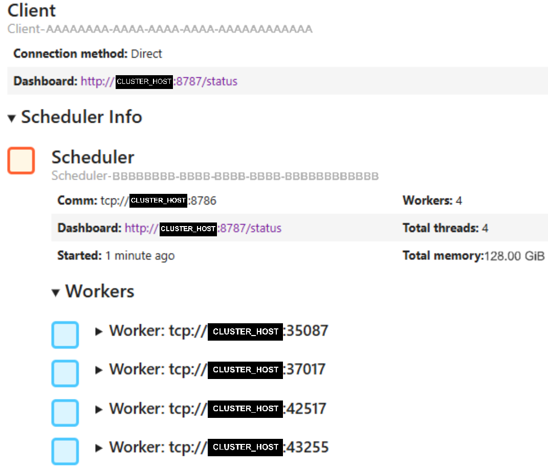

Finally, execute the pipeline by calling the seg_labels.compute() method.

python

_ = seg_labels.compute()

Note

The pipeline’s elapsed time depends on the computing resources of the cluster and the size of the input image. It can even take a couple of hours to process a Whole Slide Image (WSI).

3.5. Viewing cluster statistics

Use the address shown by the client under “Dashboard” to monitor the cluster’s status while the process is running. This tool allows us to visualize the task’s progress and overall usage of the cluster’s resources.

Tip

The Dashboard can be accessed through http://CLUSTER_HOST:8787/status. Note that the port $8787$ is used by default; however, in case that port $8787$ is already in use a random port will be generated. The port can be specified when starting the scheduler with the --dashboard-address argument.

Note

This dashboard may not show the usage of the GPUs, for what the nvidia-smi command can be used instead.

3.6. Shutting down the `dask.distributed` cluster

After the whole process has finished, execute the command below to shut down the cluster. This will safely terminate the scheduler process and all workers associated with it.

python

client.shutdown()

4. Examine output segmentation

The output of this pipeline is stored in Zarr format and can be opened with any software supporting it. Some image analysis that have support for opening Zarr files are QPath, Fiji/ImageJ, napari, vizarr, etc.

4.1. Loading regions from disk with `dask`

A similar approach to opening the input image can be used to load the resulting segmentation output in Python or jupyter.

python

seg_labels = da.from_zarr(
    "/path/to/segmentation/output.zarr",
    component="0/0"
)

Tip

It is recommended to examine relatively small regions of the input image and resulting segmentation instead of the whole extent of the images to prevent running out of memory.

Example of examination of a 512x512 pixels region of interest

In the following code a region of interest (ROI) of size $256\times256$ pixels at pixel coordinates ($512$, $512$) is examined.

python

import matplotlib.pyplot as plt

plt.imshow(im[0, :, 0, 512:512 + 256, 512:512 + 256].transpose(1, 2, 0))
plt.imshow(seg_labels[512:512 + 256, 512:512 + 256], alpha=0.5)
plt.show()

The input image is assumed to be stored following the OME specification; therefore, its axes require to be transposed before calling the imshow function.

5. Results

This section presents a set of experimental results of the proposed approach applied to a test image on different configurations. The test image used in these experiments can be downloaded with the fetch_wholeslide_example_data function from the micro_sam.sample_data module. The example image was converted using bioformats2raw with different chunk sizes for comparison purposes. The dask.distributed cluster used for these experiments consists of a scheduler and four workers. Each worker has $32$ GB of RAM and is assigned a MIG instance with $20$ GB of VRAM from a NVIDIA A100-SXM4-80GB GPU. The example image is a $4096\times4096$ pixels crop from a WSI.

Multiple values of tile shape were tested to capture different use-cases. For example, small objects (e.g. cells) are better segmented by using relatively small tiles ($256\times256$ pixels), while groups of objects are better captured with large tile shapes (e.g. groups of cells at $512\times512$ pixels, or even tissue at $1024\times1024$ pixels).

5.1. Comparing both pipelines

Figure 1 shows the elapsed time taken to segment the sample image using the baseline and the proposed approaches when varying the tile shape parameter. In Figure 2, the count of the objects segmented with the different configurations is shown.

Boxplot
Bars

Figure 1: Elapsed time for segmenting a $4096\times4096$ pixels sample image with different *tile shapes* ($1024\times1024$, $512\times512$, and $256\times256$ pixels), using the baseline pipeline and the proposed distributed pipeline.

Figure 2: Count of segmented objects in a $4096\times4096$ pixels sample image obtained with different *tile shapes* ($1024\times1024$, $512\times512$, and $256\times256$ pixels) using the baseline pipeline and the proposed distributed pipeline.

According to the experimental results, the proposed distributed approach offers an average speed-up of $8.10$ times compared with the baseline approach, and an average increment of $5.3 \%$ of objects segmented. The increment on segmented objects is due to edge effects that cause objects in adjacent chunks be labeled with different indices. However, there exist tools for handling such edge effects which commonly involve adding overlapping pixels between chunks and relabeling objects in edge regions.

5.2. Experimenting with input’s chunk sizes

The size of the chunks handled to each worker also has an effect on the segmentation time. To capture different cases, the sample image was re-chunked to different chunk sizes: $2048\times2048$, and $1024\times1024$ pixels per chunk. The time taken to segment the sample image and the count of segmented objects was measured for the different combinations of input’s chunk sizes and segmentation tile shapes. The results are presented in Figure 3 and Figure 4, respectively.

Boxplot
Bars

Figure 3: Elapsed time for segmenting a $4096\times4096$ pixels sample image using the proposed distributed pipeline for different combinations of input’s *chunk size* and *tile shape*.

Figure 4: Count of segmented objects in a $4096\times4096$ pixels sample image using the proposed distributed pipeline for different combinations of input’s *chunk size* and *tile shape*.

The experimental results show that overall segmentation time is minimal when the input’s chunk sizes matches the segmentation tile shape. The count of segmented objects is also greater in small chunks compared to larger chunks. However, this is related to single objects labeled with distinct indices by different workers. This problem can be solved in a similar manner as mentioned in Section 5.1 by using overlapping pixels and relabeling algorithms.

5.3. Closing remarks

This guide introduced a pipeline for scaling-up inference with deep learning methods to a WSI scale applying parallel computing. The experiments have shown a relevant improvement in terms of computation time of the proposed distributed approach with respect to the baseline’s sequential computing. While the computational experiments have been applied only on a sub-image extracted from a WSI, this approach can be similarly applied to the complete extent of a WSI.

1. Overview

1.1. Segmentation methods

1.2. Distributed segmentation approach

2. Dask distributed cluster

2.1. Requesting an interactive job

2.2. Configuring a dask.distributed cluster

2.3. Starting the cluster’s scheduler

2.4. Starting the cluster’s workers

3. Distributed segmentation

3.1. Encapsulating micro-sam segmentation function

3.2. Opening an image with dask

3.2.1. Convert input image to Zarr (Optional)

3.2.2. Re-chunk tiles to contain all channels

3.3. Generating a distributed process for lazy computation

3.4. Submitting graph for computation

3.5. Viewing cluster statistics

3.6. Shutting down the dask.distributed cluster

4. Examine output segmentation

4.1. Loading regions from disk with dask

5. Results

5.1. Comparing both pipelines

5.2. Experimenting with input’s chunk sizes

5.3. Closing remarks

2. Dask `distributed` cluster

2.2. Configuring a `dask.distributed` cluster

3.1. Encapsulating `micro-sam` segmentation function

3.2. Opening an image with `dask`

3.6. Shutting down the `dask.distributed` cluster

4.1. Loading regions from disk with `dask`