Working with scikit-image
Last updated on 2025-03-31 | Edit this page
Estimated time: 120 minutes
Overview
Questions
- How can the scikit-image Python computer vision library be used to work with images?
Objectives
- Read and save images with imageio.
- Display images with Matplotlib.
- Understand RGB vs Multichannel bioimages
- Extract sub-images using array slicing.
We have covered much of how images are represented in computer software. In this episode we will learn some more methods for accessing and changing digital images.
First, import the packages needed for this episode
Reading and displaying images
Imageio provides intuitive functions for reading and writing (saving) images. All of the popular image formats, such as BMP, PNG, JPEG, and TIFF are supported, along with several more esoteric formats. Check the Supported Formats docs for a list of all formats. Matplotlib provides a large collection of plotting utilities.
Let us examine a simple Python program to load, display, and save an image to a different format.
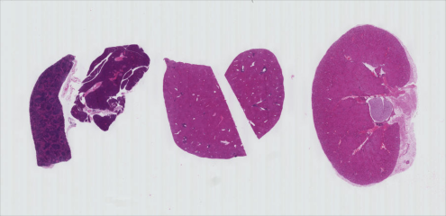
The image we will be using for much of this course is hosted on the JAX public image data repository and was used in a published manuscript from 2023. For simplicity, a lower resolution (smaller) version of the image has been converted to the more universal TIFF format for this workshop.
Here are the first few lines:
PYTHON
"""Python program to open, display, and save an image."""
# read image
he_image = iio.imread(uri="data/he_scale3.tif")
We use the iio.imread() function to read a TIFF image
entitled he_scale3. Imageio reads the image, converts
it from TIFF into a NumPy array, and returns the array; we save the
array in a variable named he_image.
Next, we will do something with the image:
Once we have the image in the program, we first call
fig, ax = plt.subplots() so that we will have a fresh
figure with a set of axes independent from our previous calls. Next we
call ax.imshow() in order to display the image.
Saving images
This line,
iio.imwrite(uri="data/he_converted.jpg",image=he_image),
writes the image to a file named he_converted.jpg in the
data/ directory. The imwrite() function
automatically determines the type of the file, based on the file
extension we provide. In this case, the .tif extension
causes the image to be saved as a TIFF, and the .jpg
extension causes the image to be saved as a JPG. Using Finder or File
Explorer, check out the size difference between these two files. As we
discussed in the Image Basics
episode, JPG is performing a lossy compression to save a smaller
file.
Metadata, revisited
Remember, as mentioned in the previous section, images saved with
imwrite() will not retain all metadata associated with the
original image that was loaded into Python! If the image metadata
is important to you, be sure to always keep an unchanged copy of
the original image!
Extensions do not always dictate file type
The iio.imwrite() function automatically uses the file
type we specify in the file name parameter’s extension. Note that this
is not always the case. For example, if we are editing a document in
Microsoft Word, and we save the document as paper.pdf
instead of paper.docx, the file is not saved as a
PDF document.
Named versus positional arguments
When we call functions in Python, there are two ways we can specify the necessary arguments. We can specify the arguments positionally, i.e., in the order the parameters appear in the function definition, or we can use named arguments.
For example, the iio.imwrite() function
definition specifies two parameters, the resource to save the image
to (e.g., a file name, an http address) and the image to write to disk.
So, we could save the chair image in the sample code above using
positional arguments like this:
iio.imwrite("data/he_converted.jpg", he_image)
Since the function expects the first argument to be the file name,
there is no confusion about what "data/he_converted.jpg"
means. The same goes for the second argument.
The style we will use in this workshop is to name each argument, like this:
iio.imwrite(uri="data/he_converted.jpg", image=he_image)
This style will make it easier for you to learn how to use the variety of functions we will cover in this workshop.
Converting colour images to grayscale
It is often easier to work with grayscale images, which have a single
channel, instead of colour images, which have three channels.
scikit-image offers the function ski.color.rgb2gray() to
achieve this. This function adds up the three colour channels in a way
that matches human colour perception, see the
scikit-image documentation for details. It returns a grayscale image
with floating point values in the range from 0 to 1. We can use the
function ski.util.img_as_ubyte() in order to convert it
back to the original data type and the data range back 0 to 255. Note
that it is often better to use image values represented by floating
point values, because using floating point numbers is numerically more
stable.
Colour and color
The Carpentries generally prefers UK English spelling, which is why
we use “colour” in the explanatory text of this lesson. However,
scikit-image contains many modules and functions that include the US
English spelling, color. The exact spelling matters here,
e.g. you will encounter an error if you try to run
ski.colour.rgb2gray(). To account for this, we will use the
US English spelling, color, in example Python code
throughout the lesson. You will encounter a similar approach with
“centre” and center.
PYTHON
"""Python script to load a color image as grayscale."""
# convert to grayscale and display
he_gray = ski.color.rgb2gray(he_image)
fig, ax = plt.subplots()
ax.imshow(he_gray, cmap="gray")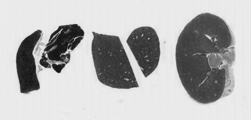
It may not be immediately obvious why we would want to do this, but we will see later in the workshop that converting the image to a single value is very helpful for downstream processing such as segmentation.
Loading images with imageio: Pixel type and depth
When loading certain image types in Python, the pixel values are
stored as 8-bit integer numbers that can take values in the range 0-255.
However, pixel values may also be stored with other types and ranges.
For example, some scikit-image functions return the pixel values as
floating point numbers in the range 0-1. The type and range of the pixel
values are important for the colorscale when plotting, and for masking
and thresholding images as we will see later in the lesson. If you are
unsure about the type of the pixel values, you can inspect it with
print(image.dtype). For the example above, you should find
that it is dtype('uint8') indicating 8-bit integer
numbers.
Multichannel images
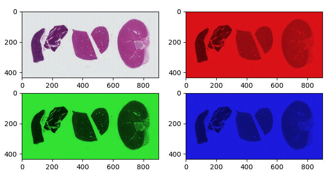
In the Image Basics episode we discussed how color is represented by three numbers in RGB images. The H&E image we have been using is an RGB image. The tissue was stained with hematoxylin (blue) and eosin (pink), but if we split apart the RGB color channels, each one isn’t particularly useful in identifying that staining:
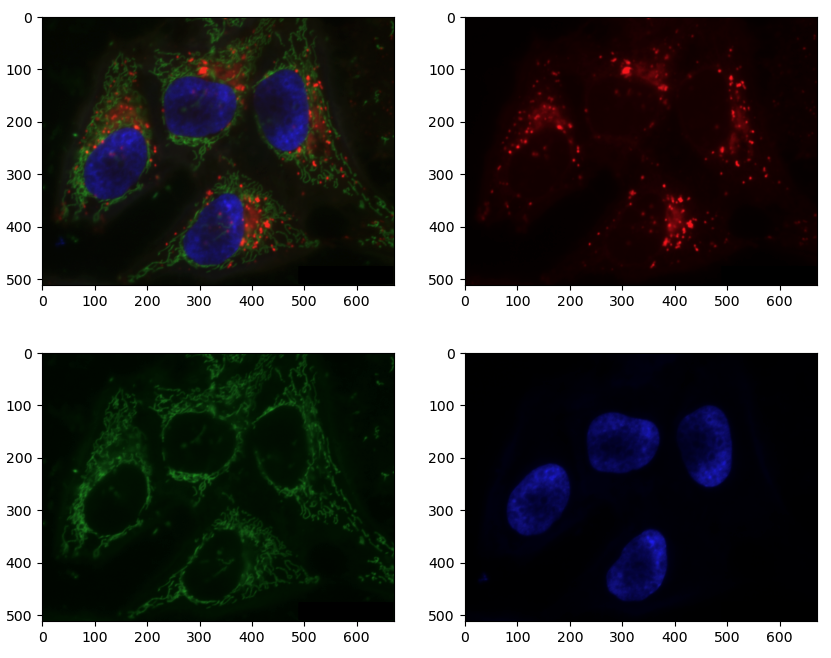
In contrast, the image of HeLa cells is a multichannel image. We can conveniently read it and view it using the same functions as RGB, since it’s still 8bit with three channels. But in reality, those channels represent fluorescence of three different parts of the cell: lysosomes, mitochondria and nucleus. Currently, the lysosomes are marked in red, mitochondria in green, and nucleus in blue, but it doesn’t really matter what color each is represented by. It’s often more useful to view multichannel images one channel at a time.
PYTHON
cells = iio.imread(uri="data/hela-cells-8bit.tif")
nuclei = cells[:,:,2]
mitochondria = cells[:,:,1]
fig, ax = plt.subplots(ncols=2)
ax[0].imshow(nuclei)
ax[1].imshow(mitochondria, vmax=255)Plotting single channel images (cmap, vmin, vmax)
Compared to a colour image, a grayscale image or a single channel
contains only a single intensity value per pixel. When we plot such an
image with ax.imshow, Matplotlib uses a colour map, to
assign each intensity value a colour. The default colour map is called
“viridis” and maps low values to purple and high values to yellow. We
can instruct Matplotlib to map low values to black and high values to
white instead, by calling ax.imshow with
cmap="gray". The
documentation contains an overview of pre-defined colour maps.
Furthermore, Matplotlib determines the minimum and maximum values of
the colour map dynamically from the image, by default. That means that
in an image where the minimum is 64 and the maximum is 192, those values
will be mapped to black and white respectively (and not dark gray and
light gray as you might expect). If there are defined minimum and
maximum vales, you can specify them via vmin and
vmax to get the desired output.
If you forget about this, it can lead to unexpected results.
Access via slicing
As noted in the previous lesson scikit-image images are stored as NumPy arrays, so we can use array slicing to select rectangular areas of an image. Then, we can save the selection as a new image, change the pixels in the image, and so on. It is important to remember that coordinates are specified in (ry, cx) order and that colour values are specified in (r, g, b) order when doing these manipulations.
Consider our H&E image, and suppose we want to create a sub-image of just one of the tissue sections.
Using matplotlib.pyplot.imshow we can determine the
coordinates of the corners of the area we wish to extract by hovering
the mouse near the points of interest and noting the coordinates
(remember to run %matplotlib widget first if you haven’t
already). If we do that, we might settle on a rectangular area with an
upper-left coordinate of (625, 45) and a lower-right coordinate
of (850, 380), as shown in this version of the HeLa
picture:
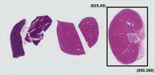
Note that the coordinates in the preceding image are specified in
(cx, ry) order. Now if our entire HeLa cell image is stored as
a NumPy array named image, we can create a new image of the
selected region with a statement like this:
clip = image[45:381, 625:851, :]
Our array slicing specifies the range of y-coordinates or rows first,
45:381, and then the range of x-coordinates or columns,
625:851. Note we go one beyond the maximum value in each
dimension, so that the entire desired area is selected, because the
sliced area does not include the upper bound index. The third part of
the slice, :, indicates that we want all three colour
channels in our new image.
A script to create the subimage would start by loading the image:
PYTHON
"""Python script demonstrating image modification and creation via NumPy array slicing."""
# load and display original image
he_image = iio.imread(uri="data/he_scale3.tif")
fig, ax = plt.subplots()
ax.imshow(he_image)Then we use array slicing to create a new image with our selected area and then display the new image.
PYTHON
# extract, display, and save sub-image
kidney = he_image[45:381, 625:851, :]
fig, ax = plt.subplots()
ax.imshow(kidney)
iio.imwrite(uri="data/kidney.tif", image=kidney)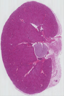
Challenge
Practicing with slices (10 min) Repeat the above exercise for the leftmost tissue section in the H&E image.
Solution Here is the completed Python program to select only the leftmost cell in the image
“““Python script to extract a sub-image containing only the leftmost cell in an existing image.”“”
PYTHON
# load and display original image
he_image = iio.imread(uri="data/he_scale3.tif")
fig, ax = plt.subplots()
ax.imshow(he_image)

# extract and display sub-image
tissue = he_image[80:351, 50:311, :]
fig, ax = plt.subplots()
ax.imshow(tissue)


# save sub-image
iio.imwrite(uri="data/tissue.jpg", image=tissue)- Images are read from disk with the
iio.imread()function. - We create a window that automatically scales the displayed image
with Matplotlib and calling
imshow()on the global figure object. - Colour images can be transformed to grayscale using
ski.color.rgb2gray()or, in many cases, be read as grayscale directly by passing the argumentmode="L"toiio.imread(). - Array slicing can be used to extract sub-images or modify areas of
images, e.g.,
clip = image[45:381, 625:851, :]. - Metadata is not retained when images are loaded as NumPy arrays
using
iio.imread().