Thresholding

Estimated time: 110 minutes

Overview

Questions

• How can we use thresholding to produce a binary image?

Objectives

• Explain what thresholding is and how it can be used.
• Use histograms to determine appropriate threshold values to use for the thresholding process.
• Apply simple, fixed-level binary thresholding to an image.
• Explain the difference between using the operator > or the operator < to threshold an image represented by a NumPy array.
• Describe the shape of a binary image produced by thresholding via > or <.
• Explain when Otsu’s method for automatic thresholding is appropriate.
• Apply automatic thresholding to an image using Otsu’s method.
• Use the np.count_nonzero() function to count the number of non-zero pixels in an image.

In this episode, we will learn how to use scikit-image functions to apply thresholding to an image. Thresholding is a type of image segmentation, where we change the pixels of an image to make the image easier to analyze. In thresholding, we convert an image from colour or grayscale into a binary image, i.e., one that is simply black and white. Most frequently, we use thresholding as a way to select areas of interest of an image, while ignoring the parts we are not concerned with. In this episode, we will learn how to use scikit-image functions to perform thresholding. Then, we will use the masks returned by these functions to select the parts of an image we are interested in.

First, import the packages needed for this episode

---

PYTHON

import imageio.v3 as iio
import ipympl
import matplotlib.pyplot as plt
import numpy as np
import skimage as ski

%matplotlib widget

Simple thresholding

---

We will start with the image of four hela cells:

PYTHON

# load the image
cells = iio.imread(uri="data/hela-cells-8bit.tif")

fig, ax = plt.subplots()
ax.imshow(cells)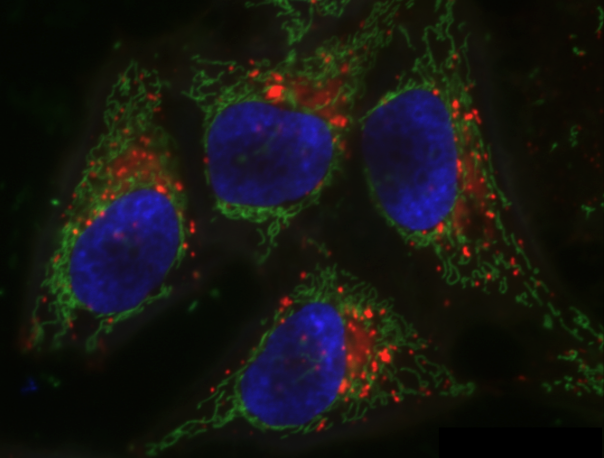

Now suppose we want to select only the nuclei of the image. In other words, we want to leave the pixels belonging to the nuclei tissue “on,” while turning the rest of the pixels “off,” by setting their colour channel values to zeros. The scikit-image library has several different methods of thresholding. We will start with the simplest version, which involves an important step of human input. Specifically, in this simple, fixed-level thresholding, we have to provide a threshold value t.

The process works like this. First, we will load the original image, convert it to grayscale or select one of the channels, and de-noise it as in the Blurring Images episode.

Since the nuclei are marked in this multichannel image by high values of the blue channel, we can select just the blue channel instead of converting the whole image to grayscale.

PYTHON

# get nuclei channel
blue_channel = cells[:,:,2]

# blur the image to denoise
blurred_nuclei = ski.filters.gaussian(blue_channel, sigma=1.0)

fig, ax = plt.subplots()
ax.imshow(blurred_nuclei, cmap="gray")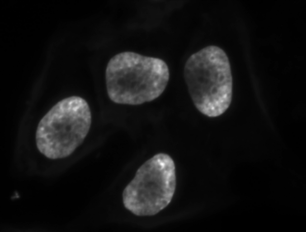

Denoising an image before thresholding

In practice, it is often necessary to denoise the image before thresholding, which can be done with one of the methods from the Blurring Images episode.

It may also be helpful to perform other types of denoising or background subtraction, such as rolling ball or tophat transforms.

Next, we would like to apply the threshold t such that pixels with grayscale values on one side of t will be turned “on”, while pixels with grayscale values on the other side will be turned “off”. How might we do that? Remember that grayscale images contain pixel values in the range from 0 to 1, so we are looking for a threshold t in the closed range [0.0, 1.0]. We see in the image that the nuclei are “lighter” than the black background. One way to determine a “good” value for t is to look at the grayscale histogram of the image and try to identify what grayscale ranges correspond to the staining in the image or the background.

The histogram can be produced as in the Creating Histograms episode.

PYTHON

# create a histogram of the blurred nuclei image
histogram, bin_edges = np.histogram(blurred_nuclei, bins=256, range=(0.0, 1.0))

fig, ax = plt.subplots()
ax.plot(bin_edges[0:-1], histogram)
ax.set_title("Grayscale Histogram")
ax.set_xlabel("grayscale value")
ax.set_ylabel("pixels")
ax.set_xlim(0, 1.0)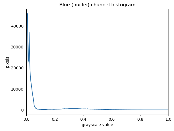

Since the image has a black background, most of the pixels in the image have low values. This corresponds nicely to what we see in the histogram: there is a peak around 0. If we want to select the fluorescing nuclei and not the background, we want to turn off the black background pixels, while leaving the pixels for the nuclei turned on. So, we should choose a value of t somewhere higher the large peak and turn pixels below that value “off”. Let us choose t=0.1.

To apply the threshold t, we can use the NumPy comparison operators to create a mask. Here, we want to turn “on” all pixels which have values bigger than the threshold, so we use the greater operator > to compare the blurred_image to the threshold t. The operator returns a mask, that we capture in the variable binary_mask. It has only one channel, and each of its values is either 0 or 1. The binary mask created by the thresholding operation can be shown with ax.imshow, where the False entries are shown as black pixels (0-valued) and the True entries are shown as white pixels (1-valued).

PYTHON

# create a mask based on the threshold
t = 0.1
binary_mask = blurred_nuclei > t

fig, ax = plt.subplots()
ax.imshow(binary_mask, cmap="gray")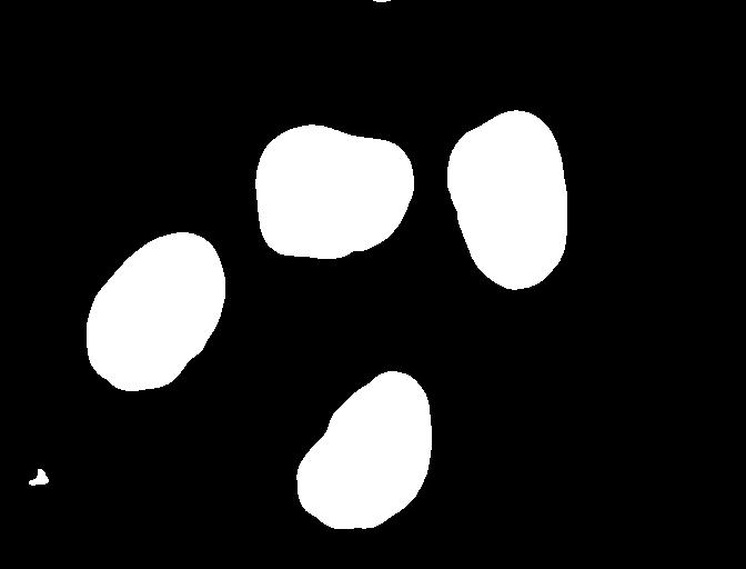

You can see that the areas where the staining was in the original area are now white, while the rest of the mask image is black.

What makes a good threshold?

As is often the case, the answer to this question is “it depends”. In the example above, we could have just switched off all the white background pixels by choosing t=1.0, but this would leave us with some background noise in the mask image. On the other hand, if we choose too low a value for the threshold, we could lose some of the staining that as too light. You can experiment with the threshold by re-running the above code lines with different values for t. In practice, it is a matter of domain knowledge and experience to interpret the peaks in the histogram so to determine an appropriate threshold. The process often involves trial and error, which is a drawback of the simple thresholding method. Below we will introduce automatic thresholding, which uses a quantitative, mathematical definition for a good threshold that allows us to determine the value of t automatically. It is worth noting that the principle for simple and automatic thresholding can also be used for images with pixel ranges other than [0.0, 1.0]. For example, we could perform thresholding on pixel intensity values in the range [0, 255] as we have already seen in the Working with scikit-image episode.

We can now apply the binary_mask to the original coloured image as we have learned in the Drawing and Bitwise Operations episode. What we are left with is only the stained tissue from the original.

PYTHON

# use the binary_mask to select the "interesting" part of the image
foreground = cells.copy()
foreground[~binary_mask] = 0

fig, ax = plt.subplots()
ax.imshow(foreground)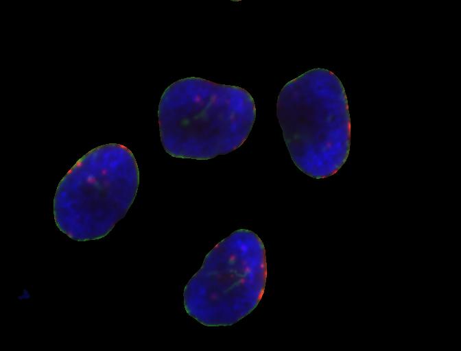

Code cheatsheet for “More practice with simple thresholding”:

PYTHON

import imageio.v3 as iio
import ipympl
import matplotlib.pyplot as plt
import numpy as np
import skimage as ski
%matplotlib widget

# Read in image (from the uri path to the image file)
image = iio.imread(uri)
# create grayscale image or select single channel (where c is the index of the channel)
channel = ski.color.rgb2gray(image) # or channel=image[:,:,c]
# Blur image
blurred_image = skimage.filters.gaussian(channel, sigma=1.0)

# Create and display image
histogram, bin_edges = np.histogram(blurred_image, bins=256, range=(0.0,1.0))
fig,ax = plt.subplots()
plt.plot(bin_edges[0:-1], histogram)
plt.title("Channel histogram")
plt.xlabel("pixel value")
plt.ylabel("pixels")
plt.xlim(0, 1.0)

# Threshold image, keeping pixels with value > t
binary_mask = blurred_image > t

# Plot threshold image
fig, ax = plt.subplots()
plt.imshow(binary_mask, cmap="gray")

# Copy image so we don't change the original
foreground = image.copy()

# Turn off all the pixels that are not our thresholded foreground
foreground[~binary_mask] = 0

# Display the image with only foreground pixels
fig, ax = plt.subplots()
plt.imshow(foreground)

More practice with simple thresholding (20 min)

Now, it is your turn to practice. Suppose we want to use simple thresholding to select only the tissue sections from the image data/he-scale3.tif:

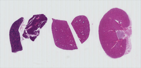
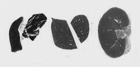
As in the Creating Histograms episode, we will use a grayscale version of the image, since the individual RGB channels are not informative on their own.

Show me the solution

The histogram for the grayscale of the H&E image can be shown with

PYTHON

# load the image
he_image = iio.imread(uri="data/he_scale3.tif")

# convert the image to grayscale
he_gray = ski.color.rgb2gray(he_image)

# blur the image to denoise
he_blurred = ski.filters.gaussian(he_gray, sigma=1.0)

# create a histogram of the blurred grayscale image
histogram, bin_edges = np.histogram(he_blurred, bins=256, range=(0.0, 1.0))

fig, ax = plt.subplots()
ax.plot(bin_edges[0:-1], histogram)
ax.set_title("Grayscale Histogram")
ax.set_xlabel("grayscale value")
ax.set_ylabel("pixels")
ax.set_xlim(0, 1.0)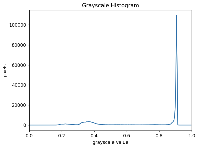

We can see a large spike around 0.9, and a very low bump around 0.2-0.4. The spike near 0.9 represents the lighter background, and the bump around 0.2-0.4 represents the darker tissue sections. So it seems like a value between the two would be a good choice. Let’s choose t=0.8.

More practice with simple thresholding (20 min) (continued)

Next, create a mask to turn the pixels below the threshold t on and pixels above the threshold t off. Note that unlike the image with a black background we used above, here the peak for the background colour is lighter than the foreground objects or nuclei. Therefore, change the comparison operator greater > to less than < to create the appropriate mask. Then apply the mask to the image and view the thresholded image. If everything works as it should, your output should show only the coloured tissue sections on a black background.

Show me the solution

Here are the commands to create and view the binary mask

PYTHON

# create a mask based on the threshold
t = 0.8
binary_mask = he_blurred < t

fig, ax = plt.subplots()
ax.imshow(binary_mask, cmap="gray")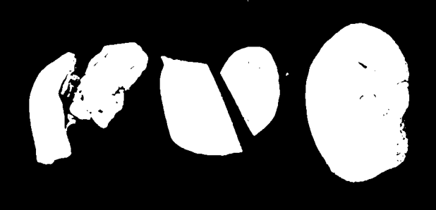

And here are the commands to apply the mask and view the thresholded image

PYTHON

# use the binary_mask to select the "interesting" part of the image
foreground = he_image.copy()
foreground[~binary_mask] = 0

fig, ax = plt.subplots()
ax.imshow(foreground)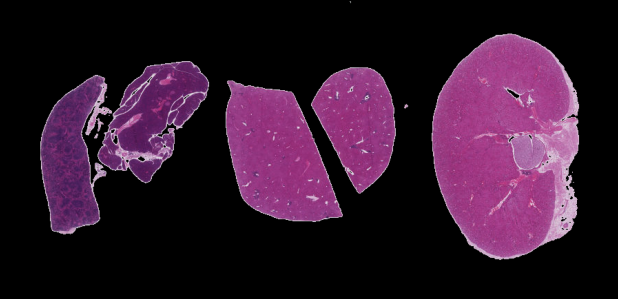

Automatic thresholding

---

The downside of the simple thresholding technique is that we have to make an educated guess about the threshold t by inspecting the histogram. There are also automatic thresholding methods that can determine the threshold automatically for us. One such method is Otsu’s method. It is particularly useful for situations where the grayscale histogram of an image has two peaks that correspond to background and objects of interest. Other automated methods might work better depending on the shape of the histogram.

Let’s apply automated thresholding methods to identify the nuclei in the HeLa cells image:

PYTHON

cells = iio.imread(uri="data/hela-cells-8bit.tif")

# select only the nuclei channel
blue_channel = cells[:,:,2]

# blur the image to denoise
blurred_image = ski.filters.gaussian(blue_channel, sigma=1.0)

# show the histogram of the blurred image
histogram, bin_edges = np.histogram(blurred_image, bins=256, range=(0.0, 1.0))
fig, ax = plt.subplots()
ax.plot(bin_edges[0:-1], histogram)
ax.set_title("Blue (nuclei) channel histogram")
ax.set_xlabel("pixel value")
ax.set_ylabel("pixel count")
ax.set_xlim(0, 1.0)

The histogram has a significant peak around 0 and then a broader “hill” around 0.3. Looking at the grayscale image, we can identify the peak at 0 with the background and the broader hill around 0.3 with the foreground. The mathematical details of how automated thresholders work are complicated (see the scikit-image documentation if you are interested), but the outcome is that Otsu’s method finds a threshold value between the two peaks of a grayscale histogram which might correspond well to the foreground and background depending on the data and application.

Instructor Note

The histogram may prompt questions from learners about the interpretation of the peaks and the broader region. The focus here is on the separation of background and foreground pixel values. We note that Otsu’s method does not work very well as the foreground pixel values are more distributed. These examples could be augmented with a discussion of unimodal, bimodal, and multimodal histograms. While these points can lead to fruitful considerations, the text in this episode attempts to reduce cognitive load and deliberately simplifies the discussion.

The ski.filters.threshold_otsu() function can be used to determine the threshold automatically via Otsu’s method. Then NumPy comparison operators can be used to apply it as before. Here are the Python commands to determine the threshold t with Otsu’s method.

PYTHON

# perform automatic thresholding
t = ski.filters.threshold_otsu(blurred_image)
print("Found automatic threshold t = {}.".format(t))

OUTPUT

Found automatic threshold t = 0.4172454549881862.

For this image, after blurring with the chosen sigma of 1.0, the computed threshold value is 0.21. Now we can create a binary mask with the comparison operator >. As we have seen before, pixels above the threshold value will be turned on, those below the threshold will be turned off.

PYTHON

# create a binary mask with the threshold found by Otsu's method
binary_mask = blurred_image > t

fig, ax = plt.subplots()
ax.imshow(binary_mask, cmap="gray")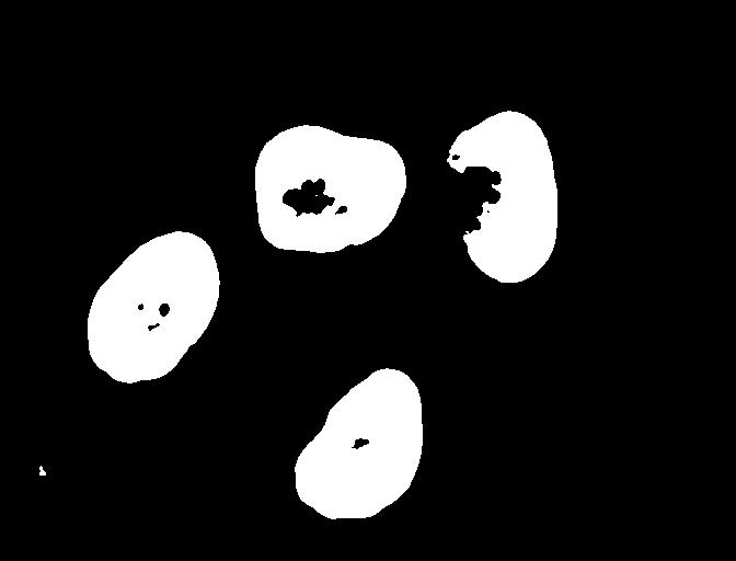

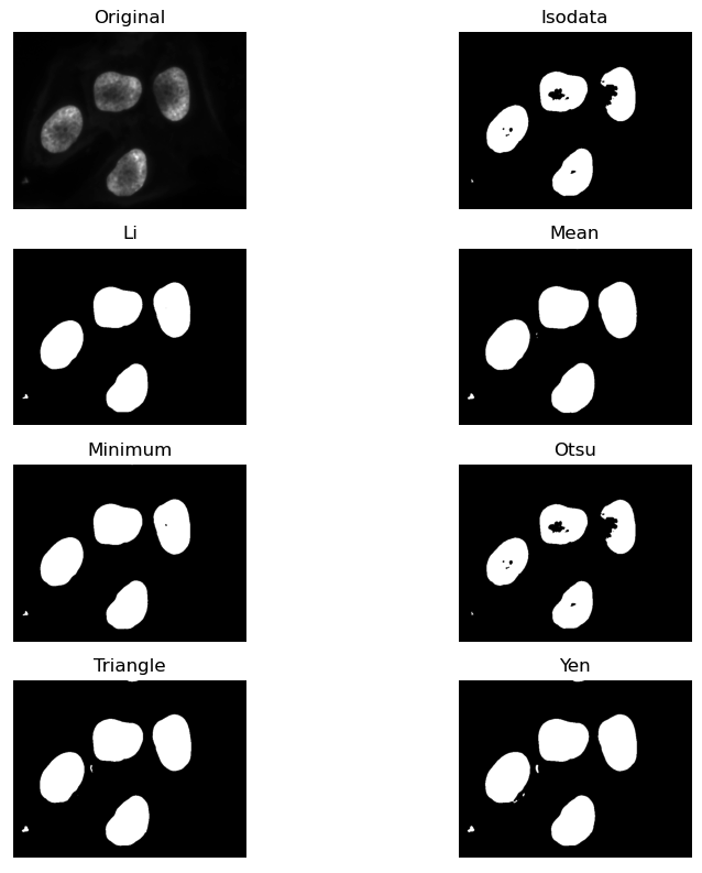
Otsu’s method generates a fairly conservative mask on this image, meaning that the threshold was fairly high and less of the foreground is kept by the mask. There may be other automated thresholders that work better in this application. Scikit image provides a method that can give a visual test of all of them at once.

PYTHON

fig, ax = ski.filters.try_all_threshold(blurred_image, figsize=(10, 8), verbose=False)

Measuring thresholded areas

---

There are many reasons why we might want to measure the percentage or size of a thresholded foreground in an image, for instance to assess tumor percentage in a tissue section or confluence of a cell culture. Here we will use it to compare the results of different automated thresholding methods.

Write a function to calculate the percentage of thresholded foreground in the image by counting the number of nonzero (or true) pixels in the binary mask and dividing by the total count of pixels.

PYTHON

def measure_foreground(blurred_image, t):
    binary_mask = blurred_image < t
    foreground_pixels = np.count_nonzero(binary_mask)
    w = binary_mask.shape[1]
    h = binary_mask.shape[0]
    percentage = foreground_pixels / (w * h) * 100
    return(percentage)

Calculate the percentage pixels kept by the Otsu thresholding method

PYTHON

t_otsu = ski.filters.threshold_otsu(blurred_image)
percentage_otsu = measure_foreground(blurred_image, t_otsu)
print("Otsu thresholding: {:.2f}%".format(percentage_otsu))

OUTPUT

Otsu thresholding: 13.21%

Measure results of automated threshold methods

Following the pipeline from above, measure the percentage of pixels kept by two different automated threshold methods.

Solution with Triangle and Yen thresholding methods

PYTHON

t_triangle = ski.filters.threshold_li(blurred_image)
percentage_triangle = measure_foreground(blurred_image, t_triangle)
print("Li thresholding: {:.2f}%".format(percentage_triangle))

t_yen = ski.filters.threshold_yen(blurred_image)
percentage_yen = measure_foreground(blurred_image, t_yen)
print("Yen thresholding: {:.2f}%".format(percentage_yen))

OUTPUT

Li thresholding: 15.05%
Yen thresholding: 16.45%

Key Points

• Thresholding produces a binary image, where all pixels with intensities above (or below) a threshold value are turned on, while all other pixels are turned off.
• The binary images produced by thresholding are held in two-dimensional NumPy arrays, since they have only one colour value channel. They are boolean, hence they contain the values 0 (off) and 1 (on).
• Thresholding can be used to create masks that select only the interesting parts of an image, or as the first step before edge detection or finding contours.