Segmentation
Last updated on 2025-04-01 | Edit this page
Estimated time: 125 minutes
Overview
Questions
- How to extract separate objects from an image and describe these objects quantitatively.
Objectives
- Understand the term object in the context of images.
- Learn about pixel connectivity.
- Learn how Connected Component Analysis (CCA) works.
- Use CCA to produce an image that highlights every object in a different colour.
- Characterise each object with numbers that describe its appearance.
Objects
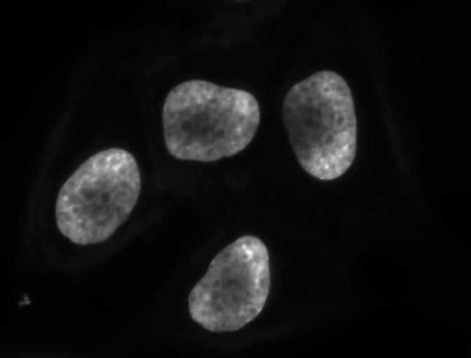
In the Thresholding episode we have covered dividing an image into foreground and background pixels. In the HeLa cells example image blue channel, we considered the coloured nuclei as foreground objects on a black background.
In thresholding we went from the original image to this version:
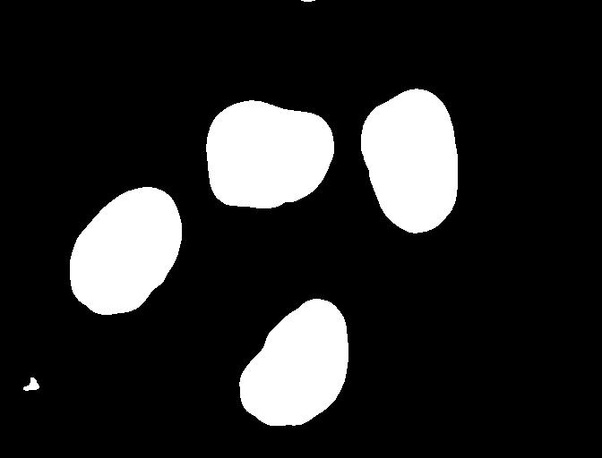
Here, we created a mask that only highlights the parts of the image
that we find interesting, the objects. All objects have pixel
value of True while the background pixels are
False.
By looking at the mask image, one can count the objects that are present in the image. But how did we actually do that, how did we decide which lump of pixels constitutes a single object?
Pixel Neighborhoods
In order to decide which pixels belong to the same object, one can exploit their neighborhood: pixels that are directly next to each other and belong to the foreground class can be considered to belong to the same object.
Let’s discuss the concept of pixel neighborhoods in more detail.
Consider the following mask “image” with 8 rows, and 8 columns. For the
purpose of illustration, the digit 0 is used to represent
background pixels, and the letter X is used to represent
object pixels foreground).
OUTPUT
0 0 0 0 0 0 0 0
0 X X 0 0 0 0 0
0 X X 0 0 0 0 0
0 0 0 X X X 0 0
0 0 0 X X X X 0
0 0 0 0 0 0 0 0
The pixels are organised in a rectangular grid. In order to
understand pixel neighborhoods we will introduce the concept of “jumps”
between pixels. The jumps follow two rules: First rule is that one jump
is only allowed along the column, or the row. Diagonal jumps are not
allowed. So, from a centre pixel, denoted with o, only the
pixels indicated with a 1 are reachable:
OUTPUT
- 1 -
1 o 1
- 1 -
The pixels on the diagonal (from o) are not reachable
with a single jump, which is denoted by the -. The pixels
reachable with a single jump form the 1-jump
neighborhood.
The second rule states that in a sequence of jumps, one may only jump
in row and column direction once -> they have to be
orthogonal. An example of a sequence of orthogonal jumps is
shown below. Starting from o the first jump goes along the
row to the right. The second jump then goes along the column direction
up. After this, the sequence cannot be continued as a jump has already
been made in both row and column direction.
OUTPUT
- - 2
- o 1
- - -
All pixels reachable with one, or two jumps form the
2-jump neighborhood. The grid below illustrates the
pixels reachable from the centre pixel o with a single
jump, highlighted with a 1, and the pixels reachable with 2
jumps with a 2.
OUTPUT
2 1 2
1 o 1
2 1 2
We want to revisit our example image mask from above and apply the
two different neighborhood rules. With a single jump connectivity for
each pixel, we get two resulting objects, highlighted in the image with
A’s and B’s.
OUTPUT
0 0 0 0 0 0 0 0
0 A A 0 0 0 0 0
0 A A 0 0 0 0 0
0 0 0 B B B 0 0
0 0 0 B B B B 0
0 0 0 0 0 0 0 0
In the 1-jump version, only pixels that have direct neighbors along
rows or columns are considered connected. Diagonal connections are not
included in the 1-jump neighborhood. With two jumps, however, we only
get a single object A because pixels are also considered
connected along the diagonals.
OUTPUT
0 0 0 0 0 0 0 0
0 A A 0 0 0 0 0
0 A A 0 0 0 0 0
0 0 0 A A A 0 0
0 0 0 A A A A 0
0 0 0 0 0 0 0 0Object counting (optional, not included in timing)
How many objects with 1 orthogonal jump, how many with 2 orthogonal jumps?
OUTPUT
0 0 0 0 0 0 0 0
0 X 0 0 0 X X 0
0 0 X 0 0 0 0 0
0 X 0 X X X 0 0
0 X 0 X X 0 0 0
0 0 0 0 0 0 0 0
1 jump
- 1
- 5
- 2
- 5
Object counting (optional, not included in timing) (continued)
2 jumps
- 2
- 3
- 5
- 2
Jumps and neighborhoods
We have just introduced how you can reach different neighboring pixels by performing one or more orthogonal jumps. We have used the terms 1-jump and 2-jump neighborhood. There is also a different way of referring to these neighborhoods: the 4- and 8-neighborhood. With a single jump you can reach four pixels from a given starting pixel. Hence, the 1-jump neighborhood corresponds to the 4-neighborhood. When two orthogonal jumps are allowed, eight pixels can be reached, so the 2-jump neighborhood corresponds to the 8-neighborhood.
Connected Component Analysis
In order to find the objects in an image (also known as
segmentation), we want to employ an operation that is called Connected
Component Analysis (CCA). This operation takes a binary image as an
input. Usually, the False value in this image is associated
with background pixels, and the True value indicates
foreground, or object pixels. Such an image can be produced, e.g., with
thresholding. Given a thresholded image, the connected component
analysis produces a new labeled image with integer pixel
values. Pixels with the same value, belong to the same object.
scikit-image provides connected component analysis in the function
ski.measure.label(). Let us add this function to the
already familiar steps of thresholding an image.
First, import the packages needed for this episode:
PYTHON
import imageio.v3 as iio
import ipympl
import matplotlib.pyplot as plt
import numpy as np
import skimage as ski

%matplotlib widget
In this episode, we will use the ski.measure.label
function to perform the CCA. For example, we want to label individual
nuclei from the HeLa cells image.
We start by generating the binary mask of the foreground of the blue (nuclei) channel of the image, as in the Thresholding episode.
PYTHON
# load the image
cells = iio.imread(uri="data/hela-cells-8bit.tif")
blue_channel = cells[:,:,2]

sigma=2.0
t=0.1
# denoise the image with a Gaussian filter
blurred_image = ski.filters.gaussian(blue_channel, sigma=sigma)
# black background so select values greater than threshod
binary_mask = blurred_image > t
We are purposefully separating out the parameters as variables for ease of editing later.
Then we call the ski.measure.label function.
PYTHON
connectivity=2
# perform connected component analysis
labeled_image, count = ski.measure.label(binary_mask,
                                        connectivity=connectivity, return_num=True)
This function has one positional argument where we pass the
binary_mask, i.e., the binary image to work on. With the
optional argument connectivity, we specify the neighborhood
in units of orthogonal jumps. For example, by setting
connectivity=2 we will consider the 2-jump neighborhood
introduced above. The function returns a labeled_image
where each pixel has a unique value corresponding to the object it
belongs to. In addition, we pass the optional parameter
return_num=True to return the maximum label index as
count.
Optional parameters and return values
The optional parameter return_num changes the data type
that is returned by the function ski.measure.label. The
number of labels is only returned if return_num is
True. Otherwise, the function only returns the labeled image.
This means that we have to pay attention when assigning the return value
to a variable. If we omit the optional parameter return_num
or pass return_num=False, we can call the function as
If we pass return_num=True, the function returns a tuple
and we can assign it as
If we used the same assignment as in the first case, the variable
labeled_image would become a tuple, in which
labeled_image[0] is the image and
labeled_image[1] is the number of labels. This could cause
confusion if we assume that labeled_image only contains the
image and pass it to other functions. If you get an
AttributeError: 'tuple' object has no attribute 'shape' or
similar, check if you have assigned the return values consistently with
the optional parameters.
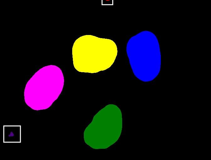
We display the labeled image like so:
We can use the function ski.color.label2rgb() to convert
the 32-bit grayscale labeled image to standard RGB colour (recall that
we already used the ski.color.rgb2gray() function to
convert to grayscale). With ski.color.label2rgb(), all
objects are coloured according to a list of colours that can be
customised. We can use the following commands to convert and show the
image:
PYTHON
# convert the label image to color image
colored_label_image = ski.color.label2rgb(labeled_image, bg_label=0)

fig, ax = plt.subplots()
ax.imshow(colored_label_image)
How does parameter choice change how many objects are in the image? (15 min)
Now, it is your turn to practice. Using the function
segment_multichannel, print out the value
count to see how many objects were found in the image.
What number of objects would you expect to get?
How does changing the sigma and threshold
values influence the result?
As you might have guessed, the return value count
already contains the number of objects found in the image. So it can
simply be printed with
But there is also a way to obtain the number of found objects from
the labeled image itself. Recall that all pixels that belong to a single
object are assigned the same integer value. The connected component
algorithm produces consecutive numbers. The background gets the value
0, the first object gets the value 1, the
second object the value 2, and so on. This means that by
finding the object with the maximum value, we also know how many objects
there are in the image. We can thus use the np.max function
from NumPy to find the maximum value that equals the number of found
objects:
Invoking the function with sigma=1.0, and
threshold=0.1, both methods will print
OUTPUT
Found 6 objects in the image.How do parameters affect output?
Raising the threshold will result in fewer objects. The lower the threshold is set, the more objects are found. More and more background noise gets picked up as objects. Larger sigmas produce binary masks with less noise and hence a smaller number of objects. Setting sigma too high bears the danger of merging objects.
You might wonder why the connected component analysis with
sigma=1.0, and threshold=0.1 finds 6 objects,
whereas we would expect only 4 objects. Where are the two additional
objects? With a bit of detective work, we can spot some small objects in
the image, for example, near the bottom left corner and top border.
For us it is clear that these small spots are artifacts and not
objects we are interested in. But how can we tell the computer? One way
to calibrate the algorithm is to adjust the parameters for blurring
(sigma) and thresholding (t), but you may have
noticed during the above exercise that it is quite hard to find a
combination that produces the right output number. In some cases,
background noise gets picked up as an object. And with other parameters,
some of the foreground objects get broken up or disappear completely.
Therefore, we need other criteria to describe desired properties of the
objects that are found.
Morphometrics - Describe object features with numbers
Morphometrics is concerned with the quantitative analysis of objects
and considers properties such as size and shape. For the example of the
images with the cells, our intuition tells us that the objects should be
of a certain size or area. So we could use a minimum area as a criterion
for when an object should be detected. To apply such a criterion, we
need a way to calculate the area of objects found by connected
components. The scikit-image library provides the function
ski.measure.regionprops to measure the properties of
labeled regions. It returns a list of RegionProperties that
describe each connected region in the images. The properties can be
accessed using the attributes of the RegionProperties data
type. Here we will use the properties "area" and
"label". You can explore the
scikit-image documentation on regionprops to learn about other
properties available.
We can get a list of areas of the labeled objects as follows:
PYTHON
# compute object features and extract object areas
np.set_printoptions(legacy='1.25')
object_features = ski.measure.regionprops(labeled_image)
object_areas = [objf["area"] for objf in object_features]
object_areas
This will produce the output
OUTPUT
[20.0, 13722.0, 14147.0, 13308.0, 12629.0, 156.0]Investigate other regionprops
Use the skimage.measure.regionprops documentation for to identify other object features. Print out some of those features.
Plot a histogram of the object area distribution (10 min)
Similar to how we determined a “good” threshold in the Thresholding episode, it is often helpful to inspect the histogram of an object property. For example, we want to look at the distribution of the object areas.
- Create and examine a histogram of the object areas
obtained with
ski.measure.regionprops. - What does the histogram tell you about the objects?
The histogram can be plotted with
PYTHON
fig, ax = plt.subplots()
ax.hist(object_areas)
ax.set_xlabel("Area (pixels)")
ax.set_ylabel("Number of objects");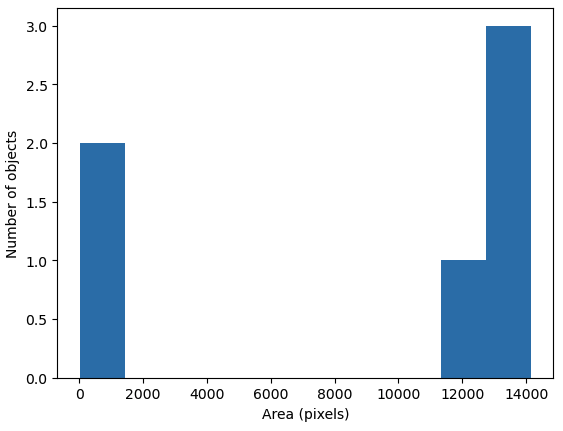
The histogram shows the number of objects (vertical axis) whose area is within a certain range (horizontal axis). The height of the bars in the histogram indicates the prevalence of objects with a certain area. The whole histogram tells us about the distribution of object sizes in the image. It is often possible to identify gaps between groups of bars (or peaks if we draw the histogram as a continuous curve) that tell us about certain groups in the image.
In this example, we can see that there are two small objects that
contain less than 2000 pixels. Then there is a group of four (1+3)
objects in the range between 10000 and 15000. For our object count, we
might want to disregard the small objects as artifacts, i.e, we want to
ignore the leftmost bar of the histogram. We could use a threshold of
8000 as the minimum area to count. In fact, the
object_areas list already tells us that there are fewer
than 200 pixels in these objects. Therefore, it is reasonable to require
a minimum area of at least 200 pixels for a detected object. In
practice, finding the “right” threshold can be tricky and usually
involves an educated guess based on domain knowledge. For example, if
you know the micrometer size of your pixel resolution and expected size
of the cells you are imaging, you could compute the expected number of
pixels per cell area and keep objects of that size.
Using functions from NumPy and other Python packages
Functions from Python packages such as NumPy are often more efficient
and require less code to write. It is a good idea to browse the
reference pages of numpy and skimage to look
for an availabe function that can solve a given task.
An elegant way to remove small objects from the image is to leverage
the ski.morphology module. It provides a function
ski.morphology.remove_small_objects that does exactly what
we are looking for. It can be applied to either a binary or a label
image and returns a mask in which all objects smaller than
min_area are excluded, i.e, their pixel values are set to
False or the background label value.
We display the resulting label image and print the number of objects:
PYTHON
color_filtered_labels = ski.color.label2rgb(filtered_labels, bg_label=0)
fig, ax = plt.subplots()
ax.imshow(color_filtered_labels)

print("Found", count, "objects in the image.")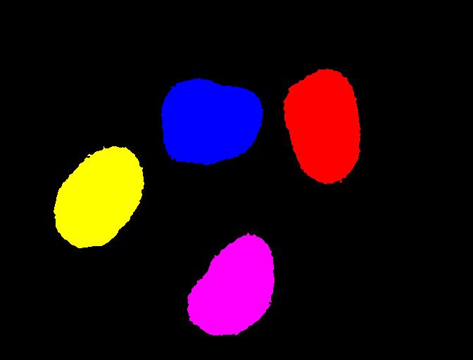
OUTPUT
Found 4 objects in the image.Note that the small objects are “gone” and we obtain the correct number of 4 objects in the image.
Segment tissue sections from an H&E image
Repeat the same steps as above for the H&E image to segment the
different tissue sections. Identify the best parameter choices for
sigma, t, connectivity, and
min_size.
Two things to remember:
The H&E image has RGB color channels that don’t mean anything on their own, so it is best to convert it to grayscale before blurring and thresholding
The H&E image has a light background, so the pixel values to turn “on” with a threshold will be less than (
<) the threshold valuet.
PYTHON
# load the image
he_image = iio.imread(uri="data/he_scale3.tif")
# convert the image to grayscale
he_gray = ski.color.rgb2gray(he_image)

sigma=1.0 # spleen sections are merged at sigma > 1
t=0.8
connectivity=2
# denoise the image with a Gaussian filter
blurred_image = ski.filters.gaussian(he_gray, sigma=sigma)
# white background so select values greater than threshod
binary_mask = blurred_image < t
# perform connected component analysis
labeled_image, count = ski.measure.label(binary_mask,
                                        connectivity=connectivity, return_num=True)

print("Found", count, "objects in the image.")
OUTPUT
Found 12 objects in the image.PYTHON
object_features = ski.measure.regionprops(labeled_image)
object_areas = [int(objf["area"]) for objf in object_features]
print(object_areas)
OUTPUT
[7, 55189, 16201, 14900, 14929, 23419, 4, 24, 2, 27, 2, 2]PYTHON
filtered_labels = ski.morphology.remove_small_objects(labeled_image, min_size=1000)
color_filtered_labels = ski.color.label2rgb(filtered_labels, bg_label=0)
fig, ax = plt.subplots()
ax.imshow(color_filtered_labels)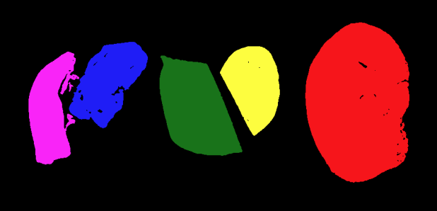
- We can use
ski.measure.labelto find and label connected objects in an image. - We can use
ski.measure.regionpropsto measure properties of labeled objects. - We can use
ski.morphology.remove_small_objectsto mask small objects and remove artifacts from an image. - We can display the labeled image to view the objects coloured by label.