Summary and Schedule

This lesson shows how to use Python and scikit-image to do basic image processing.

Prerequisites

This lesson assumes you have a working knowledge of Python and some previous exposure to the Bash shell. These requirements can be fulfilled by: a) completing a Software Carpentry Python workshop or b) completing a Data Carpentry Ecology workshop (with Python) and a Data Carpentry Genomics workshop or c) independent exposure to both Python and the Bash shell.

If you’re unsure whether you have enough experience to participate in this workshop, please read over this detailed list, which gives all of the functions, operators, and other concepts you will need to be familiar with.

Before following the lesson, please make sure you have the software and data required.

	Setup Instructions	Download files required for the lesson
Duration: 00h 00m	1. Introduction	What sort of scientific questions can we answer with image processing / computer vision? What are morphometric problems?
Duration: 00h 05m	2. Image Basics	How are images represented in digital format?
Duration: 00h 30m	3. Working with scikit-image	How can the scikit-image Python computer vision library be used to work with images?
Duration: 02h 30m	4. Drawing and Bitwise Operations	How can we draw on scikit-image images and use bitwise operations and masks to select certain parts of an image?
Duration: 04h 00m	5. Creating Histograms	How can we create grayscale and colour histograms to understand the distribution of colour values in an image?
Duration: 05h 20m	6. Blurring Images	How can we apply a low-pass blurring filter to an image?
Duration: 06h 20m	7. Thresholding	How can we use thresholding to produce a binary image?
Duration: 08h 10m	8. Connected Component Analysis	How to extract separate objects from an image and describe these objects quantitatively.
Duration: 10h 15m	Finish

The actual schedule may vary slightly depending on the topics and exercises chosen by the instructor.

Before joining the workshop or following the lesson, please complete the data and software setup described in this page.

Data

---

The example images used in this lesson are available on Zenodo. To download the data, please visit the dataset page for this workshop and click the “Download all” button. Unzip the downloaded file, and save the contents as a folder called data somewhere you will easily find it again, e.g. your Desktop or a folder you have created for using in this workshop. (The name data is optional but recommended, as this is the name we will use to refer to the folder throughout the lesson.)

Software

---

1. Check your conda distribution. On terminal (Mac) or Powershell/WSL (Windows), run:

   conda info
   mamba info

   If either command returns information, skip to creating a new environment.

2. Download and install the latest Miniforge distribution If you wish to use an existing installation, please use a new conda environment to ensure all packages are up to date.

   Instructions for Windows

   If running the conda commands on the standard Command Prompt or Powershell returns an error: 'conda' is not recognized as an internal or external command, operable program or batch file.

   Use the Miniforge Prompt in the Start menu instead.

3. Create a new environment with the necessary packages

   conda create -n imaging-workshop python=3.9 scikit-image ipympl jupyterlab -c conda-forge

   Enabling the ipympl backend in Jupyter notebooks

   This lesson uses Matplotlib features to display images, and some interactive features will be valuable. To enable the interactive tools in JupyterLab, the ipympl package is required.

   The ipympl backend can be enabled with the %matplotlib Jupyter magic. Put the following command in a cell in your notebooks (e.g., at the top) and execute the cell before any plotting commands.

   PYTHON

   %matplotlib widget

   Older JupyterLab versions

   If you are using an older version of JupyterLab, you may also need to install the labextensions manually, as explained in the README file for the ipympl package.

4. Start environment

   conda activate imaging-workshop

5. Open a Jupyter notebook:

   jupyter lab

   After Jupyter Lab has launched, click the “Python 3” button under “Notebook” in the launcher window, or use the “File” menu, to open a new Python 3 notebook.

6. To test your environment, run the following lines in a cell of the notebook:

   PYTHON

   import imageio.v3 as iio
   import matplotlib.pyplot as plt
   import skimage as ski
   
   %matplotlib widget
   
   # load an image
   image = iio.imread(uri='data/colonies-01.tif')
   
   # rotate it by 45 degrees
   rotated = ski.transform.rotate(image=image, angle=45)
   
   # display the original image and its rotated version side by side
   fig, ax = plt.subplots(1, 2)
   ax[0].imshow(image)
   ax[1].imshow(rotated)

   Upon execution of the cell, a figure with two images should be displayed in an interactive widget. When hovering over the images with the mouse pointer, the pixel coordinates and colour values are displayed below the image.

   Running Cells in a Notebook

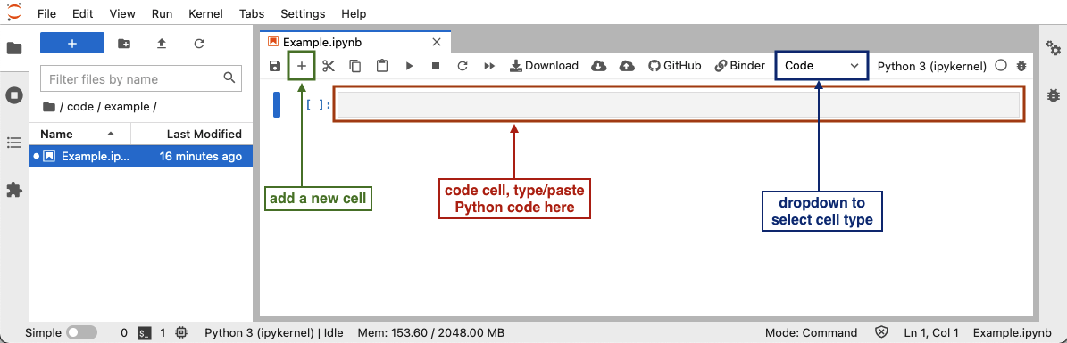   To run Python code in a Jupyter notebook cell, click on a cell in the notebook (or add a new one by clicking the + button in the toolbar), make sure that the cell type is set to “Code” (check the dropdown in the toolbar), and add the Python code in that cell. After you have added the code, you can run the cell by selecting “Run” -> “Run selected cell” in the top menu, or pressing Shift+Enter.