DEG_analysis
Last updated: 2021-08-10
Checks: 7 0
Knit directory: DO_Opioid/
This reproducible R Markdown analysis was created with workflowr (version 1.6.2). The Checks tab describes the reproducibility checks that were applied when the results were created. The Past versions tab lists the development history.
Great! Since the R Markdown file has been committed to the Git repository, you know the exact version of the code that produced these results.
Great job! The global environment was empty. Objects defined in the global environment can affect the analysis in your R Markdown file in unknown ways. For reproduciblity it’s best to always run the code in an empty environment.
The command set.seed(20200504) was run prior to running the code in the R Markdown file. Setting a seed ensures that any results that rely on randomness, e.g. subsampling or permutations, are reproducible.
Great job! Recording the operating system, R version, and package versions is critical for reproducibility.
Nice! There were no cached chunks for this analysis, so you can be confident that you successfully produced the results during this run.
Great job! Using relative paths to the files within your workflowr project makes it easier to run your code on other machines.
Great! You are using Git for version control. Tracking code development and connecting the code version to the results is critical for reproducibility.
The results in this page were generated with repository version a242947. See the Past versions tab to see a history of the changes made to the R Markdown and HTML files.
Note that you need to be careful to ensure that all relevant files for the analysis have been committed to Git prior to generating the results (you can use wflow_publish or wflow_git_commit). workflowr only checks the R Markdown file, but you know if there are other scripts or data files that it depends on. Below is the status of the Git repository when the results were generated:
Ignored files:
    Ignored:    .RData
    Ignored:    .Rhistory
    Ignored:    .Rproj.user/
    Ignored:    analysis/Picture1.png
    Ignored:    data/output/

Untracked files:
    Untracked:  analysis/DDO_morphine1_second_set_69k.stdout
    Untracked:  analysis/DO_morphine1.R
    Untracked:  analysis/DO_morphine1.Rout
    Untracked:  analysis/DO_morphine1.sh
    Untracked:  analysis/DO_morphine1.stderr
    Untracked:  analysis/DO_morphine1.stdout
    Untracked:  analysis/DO_morphine1_SNP.R
    Untracked:  analysis/DO_morphine1_SNP.Rout
    Untracked:  analysis/DO_morphine1_SNP.sh
    Untracked:  analysis/DO_morphine1_SNP.stderr
    Untracked:  analysis/DO_morphine1_SNP.stdout
    Untracked:  analysis/DO_morphine1_combined.R
    Untracked:  analysis/DO_morphine1_combined.Rout
    Untracked:  analysis/DO_morphine1_combined.sh
    Untracked:  analysis/DO_morphine1_combined.stderr
    Untracked:  analysis/DO_morphine1_combined.stdout
    Untracked:  analysis/DO_morphine1_combined_69k.R
    Untracked:  analysis/DO_morphine1_combined_69k.Rout
    Untracked:  analysis/DO_morphine1_combined_69k.sh
    Untracked:  analysis/DO_morphine1_combined_69k.stderr
    Untracked:  analysis/DO_morphine1_combined_69k.stdout
    Untracked:  analysis/DO_morphine1_combined_69k_m2.R
    Untracked:  analysis/DO_morphine1_combined_69k_m2.Rout
    Untracked:  analysis/DO_morphine1_combined_69k_m2.sh
    Untracked:  analysis/DO_morphine1_combined_69k_m2.stderr
    Untracked:  analysis/DO_morphine1_combined_69k_m2.stdout
    Untracked:  analysis/DO_morphine1_combined_weight_DOB.R
    Untracked:  analysis/DO_morphine1_combined_weight_DOB.Rout
    Untracked:  analysis/DO_morphine1_combined_weight_DOB.err
    Untracked:  analysis/DO_morphine1_combined_weight_DOB.out
    Untracked:  analysis/DO_morphine1_combined_weight_DOB.sh
    Untracked:  analysis/DO_morphine1_combined_weight_DOB.stderr
    Untracked:  analysis/DO_morphine1_combined_weight_DOB.stdout
    Untracked:  analysis/DO_morphine1_combined_weight_age.R
    Untracked:  analysis/DO_morphine1_combined_weight_age.err
    Untracked:  analysis/DO_morphine1_combined_weight_age.out
    Untracked:  analysis/DO_morphine1_combined_weight_age.sh
    Untracked:  analysis/DO_morphine1_combined_weight_age_GAMMT.R
    Untracked:  analysis/DO_morphine1_combined_weight_age_GAMMT.err
    Untracked:  analysis/DO_morphine1_combined_weight_age_GAMMT.out
    Untracked:  analysis/DO_morphine1_combined_weight_age_GAMMT.sh
    Untracked:  analysis/DO_morphine1_combined_weight_age_GAMMT_chr19.R
    Untracked:  analysis/DO_morphine1_combined_weight_age_GAMMT_chr19.err
    Untracked:  analysis/DO_morphine1_combined_weight_age_GAMMT_chr19.out
    Untracked:  analysis/DO_morphine1_combined_weight_age_GAMMT_chr19.sh
    Untracked:  analysis/DO_morphine1_cph.R
    Untracked:  analysis/DO_morphine1_cph.Rout
    Untracked:  analysis/DO_morphine1_cph.sh
    Untracked:  analysis/DO_morphine1_second_set.R
    Untracked:  analysis/DO_morphine1_second_set.Rout
    Untracked:  analysis/DO_morphine1_second_set.sh
    Untracked:  analysis/DO_morphine1_second_set.stderr
    Untracked:  analysis/DO_morphine1_second_set.stdout
    Untracked:  analysis/DO_morphine1_second_set_69k.R
    Untracked:  analysis/DO_morphine1_second_set_69k.Rout
    Untracked:  analysis/DO_morphine1_second_set_69k.sh
    Untracked:  analysis/DO_morphine1_second_set_69k.stderr
    Untracked:  analysis/DO_morphine1_second_set_SNP.R
    Untracked:  analysis/DO_morphine1_second_set_SNP.Rout
    Untracked:  analysis/DO_morphine1_second_set_SNP.sh
    Untracked:  analysis/DO_morphine1_second_set_SNP.stderr
    Untracked:  analysis/DO_morphine1_second_set_SNP.stdout
    Untracked:  analysis/DO_morphine1_second_set_weight_DOB.R
    Untracked:  analysis/DO_morphine1_second_set_weight_DOB.Rout
    Untracked:  analysis/DO_morphine1_second_set_weight_DOB.err
    Untracked:  analysis/DO_morphine1_second_set_weight_DOB.out
    Untracked:  analysis/DO_morphine1_second_set_weight_DOB.sh
    Untracked:  analysis/DO_morphine1_second_set_weight_DOB.stderr
    Untracked:  analysis/DO_morphine1_second_set_weight_DOB.stdout
    Untracked:  analysis/DO_morphine1_second_set_weight_age.R
    Untracked:  analysis/DO_morphine1_second_set_weight_age.Rout
    Untracked:  analysis/DO_morphine1_second_set_weight_age.err
    Untracked:  analysis/DO_morphine1_second_set_weight_age.out
    Untracked:  analysis/DO_morphine1_second_set_weight_age.sh
    Untracked:  analysis/DO_morphine1_second_set_weight_age.stderr
    Untracked:  analysis/DO_morphine1_second_set_weight_age.stdout
    Untracked:  analysis/DO_morphine1_weight_DOB.R
    Untracked:  analysis/DO_morphine1_weight_DOB.sh
    Untracked:  analysis/DO_morphine1_weight_age.R
    Untracked:  analysis/DO_morphine1_weight_age.sh
    Untracked:  analysis/DO_morphine_gemma.R
    Untracked:  analysis/DO_morphine_gemma.err
    Untracked:  analysis/DO_morphine_gemma.out
    Untracked:  analysis/DO_morphine_gemma.sh
    Untracked:  analysis/DO_morphine_gemma_firstmin.R
    Untracked:  analysis/DO_morphine_gemma_firstmin.err
    Untracked:  analysis/DO_morphine_gemma_firstmin.out
    Untracked:  analysis/DO_morphine_gemma_firstmin.sh
    Untracked:  analysis/DO_morphine_gemma_withpermu.R
    Untracked:  analysis/DO_morphine_gemma_withpermu.err
    Untracked:  analysis/DO_morphine_gemma_withpermu.out
    Untracked:  analysis/DO_morphine_gemma_withpermu.sh
    Untracked:  analysis/DO_morphine_gemma_withpermu_firstbatch_min.depression.R
    Untracked:  analysis/DO_morphine_gemma_withpermu_firstbatch_min.depression.err
    Untracked:  analysis/DO_morphine_gemma_withpermu_firstbatch_min.depression.out
    Untracked:  analysis/DO_morphine_gemma_withpermu_firstbatch_min.depression.sh
    Untracked:  analysis/Plot_DO_morphine1_SNP.R
    Untracked:  analysis/Plot_DO_morphine1_SNP.Rout
    Untracked:  analysis/Plot_DO_morphine1_SNP.sh
    Untracked:  analysis/Plot_DO_morphine1_SNP.stderr
    Untracked:  analysis/Plot_DO_morphine1_SNP.stdout
    Untracked:  analysis/Plot_DO_morphine1_second_set_SNP.R
    Untracked:  analysis/Plot_DO_morphine1_second_set_SNP.Rout
    Untracked:  analysis/Plot_DO_morphine1_second_set_SNP.sh
    Untracked:  analysis/Plot_DO_morphine1_second_set_SNP.stderr
    Untracked:  analysis/Plot_DO_morphine1_second_set_SNP.stdout
    Untracked:  analysis/scripts/
    Untracked:  analysis/workflow_proc.R
    Untracked:  analysis/workflow_proc.sh
    Untracked:  analysis/workflow_proc.stderr
    Untracked:  analysis/workflow_proc.stdout
    Untracked:  analysis/x.R
    Untracked:  code/cfw/
    Untracked:  code/gemma_plot.R
    Untracked:  code/reconst_utils.R
    Untracked:  data/69k_grid_pgmap.RData
    Untracked:  data/FinalReport/
    Untracked:  data/GM/
    Untracked:  data/GM_covar.csv
    Untracked:  data/GM_covar_07092018_morphine.csv
    Untracked:  data/Jackson_Lab_Bubier_MURGIGV01/
    Untracked:  data/MasterMorphine Second Set DO w DOB2.xlsx
    Untracked:  data/MasterMorphine Second Set DO.xlsx
    Untracked:  data/cc_variants.sqlite
    Untracked:  data/combined/
    Untracked:  data/first/
    Untracked:  data/founder_geno.csv
    Untracked:  data/genetic_map.csv
    Untracked:  data/gm.json
    Untracked:  data/gwas.sh
    Untracked:  data/marker_grid_0.02cM_plus.txt
    Untracked:  data/mouse_genes_mgi.sqlite
    Untracked:  data/pheno.csv
    Untracked:  data/pheno_qtl2.csv
    Untracked:  data/pheno_qtl2_07092018_morphine.csv
    Untracked:  data/pheno_qtl2_w_dob.csv
    Untracked:  data/physical_map.csv
    Untracked:  data/rnaseq/
    Untracked:  data/sample_geno.csv
    Untracked:  data/second/
    Untracked:  figure/
    Untracked:  glimma-plots/
    Untracked:  output/DO_morphine_Min.depression.png
    Untracked:  output/DO_morphine_Min.depression22222_violin_chr5.pdf
    Untracked:  output/DO_morphine_Min.depression_coefplot.pdf
    Untracked:  output/DO_morphine_Min.depression_coefplot_blup.pdf
    Untracked:  output/DO_morphine_Min.depression_coefplot_blup_chr5.png
    Untracked:  output/DO_morphine_Min.depression_coefplot_blup_chrX.png
    Untracked:  output/DO_morphine_Min.depression_coefplot_chr5.png
    Untracked:  output/DO_morphine_Min.depression_coefplot_chrX.png
    Untracked:  output/DO_morphine_Min.depression_peak_genes_chr5.png
    Untracked:  output/DO_morphine_Min.depression_violin_chr5.png
    Untracked:  output/DO_morphine_Recovery.Time.png
    Untracked:  output/DO_morphine_Recovery.Time_coefplot.pdf
    Untracked:  output/DO_morphine_Recovery.Time_coefplot_blup.pdf
    Untracked:  output/DO_morphine_Recovery.Time_coefplot_blup_chr11.png
    Untracked:  output/DO_morphine_Recovery.Time_coefplot_blup_chr4.png
    Untracked:  output/DO_morphine_Recovery.Time_coefplot_blup_chr7.png
    Untracked:  output/DO_morphine_Recovery.Time_coefplot_blup_chr9.png
    Untracked:  output/DO_morphine_Recovery.Time_coefplot_chr11.png
    Untracked:  output/DO_morphine_Recovery.Time_coefplot_chr4.png
    Untracked:  output/DO_morphine_Recovery.Time_coefplot_chr7.png
    Untracked:  output/DO_morphine_Recovery.Time_coefplot_chr9.png
    Untracked:  output/DO_morphine_Status_bin.png
    Untracked:  output/DO_morphine_Status_bin_coefplot.pdf
    Untracked:  output/DO_morphine_Status_bin_coefplot_blup.pdf
    Untracked:  output/DO_morphine_Survival.Time.png
    Untracked:  output/DO_morphine_Survival.Time_coefplot.pdf
    Untracked:  output/DO_morphine_Survival.Time_coefplot_blup.pdf
    Untracked:  output/DO_morphine_Survival.Time_coefplot_blup_chr17.png
    Untracked:  output/DO_morphine_Survival.Time_coefplot_blup_chr8.png
    Untracked:  output/DO_morphine_Survival.Time_coefplot_chr17.png
    Untracked:  output/DO_morphine_Survival.Time_coefplot_chr8.png
    Untracked:  output/DO_morphine_combine_batch_peak_violin.pdf
    Untracked:  output/DO_morphine_combined_69k_m2_Min.depression.png
    Untracked:  output/DO_morphine_combined_69k_m2_Min.depression_coefplot.pdf
    Untracked:  output/DO_morphine_combined_69k_m2_Min.depression_coefplot_blup.pdf
    Untracked:  output/DO_morphine_combined_69k_m2_Recovery.Time.png
    Untracked:  output/DO_morphine_combined_69k_m2_Recovery.Time_coefplot.pdf
    Untracked:  output/DO_morphine_combined_69k_m2_Recovery.Time_coefplot_blup.pdf
    Untracked:  output/DO_morphine_combined_69k_m2_Status_bin.png
    Untracked:  output/DO_morphine_combined_69k_m2_Status_bin_coefplot.pdf
    Untracked:  output/DO_morphine_combined_69k_m2_Status_bin_coefplot_blup.pdf
    Untracked:  output/DO_morphine_combined_69k_m2_Survival.Time.png
    Untracked:  output/DO_morphine_combined_69k_m2_Survival.Time_coefplot.pdf
    Untracked:  output/DO_morphine_combined_69k_m2_Survival.Time_coefplot_blup.pdf
    Untracked:  output/DO_morphine_coxph_24hrs_kinship_QTL.png
    Untracked:  output/DO_morphine_cphout.RData
    Untracked:  output/DO_morphine_first_batch_peak_in_second_batch_violin.pdf
    Untracked:  output/DO_morphine_first_batch_peak_in_second_batch_violin_sidebyside.pdf
    Untracked:  output/DO_morphine_first_batch_peak_violin.pdf
    Untracked:  output/DO_morphine_operm.cph.RData
    Untracked:  output/DO_morphine_second_batch_on_first_batch_peak_violin.pdf
    Untracked:  output/DO_morphine_second_batch_peak_ch6surv_on_first_batchviolin.pdf
    Untracked:  output/DO_morphine_second_batch_peak_ch6surv_on_first_batchviolin2.pdf
    Untracked:  output/DO_morphine_second_batch_peak_in_first_batch_violin.pdf
    Untracked:  output/DO_morphine_second_batch_peak_in_first_batch_violin_sidebyside.pdf
    Untracked:  output/DO_morphine_second_batch_peak_violin.pdf
    Untracked:  output/DO_morphine_secondbatch_69k_Min.depression.png
    Untracked:  output/DO_morphine_secondbatch_69k_Min.depression_coefplot.pdf
    Untracked:  output/DO_morphine_secondbatch_69k_Min.depression_coefplot_blup.pdf
    Untracked:  output/DO_morphine_secondbatch_69k_Recovery.Time.png
    Untracked:  output/DO_morphine_secondbatch_69k_Recovery.Time_coefplot.pdf
    Untracked:  output/DO_morphine_secondbatch_69k_Recovery.Time_coefplot_blup.pdf
    Untracked:  output/DO_morphine_secondbatch_69k_Status_bin.png
    Untracked:  output/DO_morphine_secondbatch_69k_Status_bin_coefplot.pdf
    Untracked:  output/DO_morphine_secondbatch_69k_Status_bin_coefplot_blup.pdf
    Untracked:  output/DO_morphine_secondbatch_69k_Survival.Time.png
    Untracked:  output/DO_morphine_secondbatch_69k_Survival.Time_coefplot.pdf
    Untracked:  output/DO_morphine_secondbatch_69k_Survival.Time_coefplot_blup.pdf
    Untracked:  output/DO_morphine_secondbatch_Min.depression.png
    Untracked:  output/DO_morphine_secondbatch_Min.depression_coefplot.pdf
    Untracked:  output/DO_morphine_secondbatch_Min.depression_coefplot_blup.pdf
    Untracked:  output/DO_morphine_secondbatch_Recovery.Time.png
    Untracked:  output/DO_morphine_secondbatch_Recovery.Time_coefplot.pdf
    Untracked:  output/DO_morphine_secondbatch_Recovery.Time_coefplot_blup.pdf
    Untracked:  output/DO_morphine_secondbatch_Status_bin.png
    Untracked:  output/DO_morphine_secondbatch_Status_bin_coefplot.pdf
    Untracked:  output/DO_morphine_secondbatch_Status_bin_coefplot_blup.pdf
    Untracked:  output/DO_morphine_secondbatch_Survival.Time.png
    Untracked:  output/DO_morphine_secondbatch_Survival.Time_coefplot.pdf
    Untracked:  output/DO_morphine_secondbatch_Survival.Time_coefplot_blup.pdf
    Untracked:  output/apr_69kchr_combined.RData
    Untracked:  output/apr_69kchr_k_loco_combined.rds
    Untracked:  output/apr_69kchr_second_set.RData
    Untracked:  output/combine_batch_variation.RData
    Untracked:  output/combined_gm.RData
    Untracked:  output/combined_gm.k_loco.rds
    Untracked:  output/combined_gm.k_overall.rds
    Untracked:  output/combined_gm.probs_36state.rds
    Untracked:  output/combined_gm.probs_8state.rds
    Untracked:  output/coxph/
    Untracked:  output/do.morphine.RData
    Untracked:  output/do.morphine.k_loco.rds
    Untracked:  output/do.morphine.probs_36state.rds
    Untracked:  output/do.morphine.probs_8state.rds
    Untracked:  output/first_batch_variation.RData
    Untracked:  output/old_temp/
    Untracked:  output/pr_69k_combined.RData
    Untracked:  output/pr_69kchr_combined.RData
    Untracked:  output/pr_69kchr_second_set.RData
    Untracked:  output/qtl.morphine.69k.out.combined.RData
    Untracked:  output/qtl.morphine.69k.out.combined_m2.RData
    Untracked:  output/qtl.morphine.69k.out.second_set.RData
    Untracked:  output/qtl.morphine.operm.RData
    Untracked:  output/qtl.morphine.out.RData
    Untracked:  output/qtl.morphine.out.combined_gm.RData
    Untracked:  output/qtl.morphine.out.combined_weight_DOB.RData
    Untracked:  output/qtl.morphine.out.combined_weight_age.RData
    Untracked:  output/qtl.morphine.out.second_set.RData
    Untracked:  output/qtl.morphine.out.second_set.weight_DOB.RData
    Untracked:  output/qtl.morphine.out.second_set.weight_age.RData
    Untracked:  output/qtl.morphine.out.weight_DOB.RData
    Untracked:  output/qtl.morphine.out.weight_age.RData
    Untracked:  output/qtl.morphine1.snpout.RData
    Untracked:  output/qtl.morphine2.snpout.RData
    Untracked:  output/second_batch_variation.RData
    Untracked:  output/second_set_apr_69kchr_k_loco.rds
    Untracked:  output/second_set_gm.RData
    Untracked:  output/second_set_gm.k_loco.rds
    Untracked:  output/second_set_gm.probs_36state.rds
    Untracked:  output/second_set_gm.probs_8state.rds
    Untracked:  output/topSNP_chr5_mindepression.csv
    Untracked:  output/zoompeak_Min.depression_9.pdf
    Untracked:  output/zoompeak_Recovery.Time_16.pdf
    Untracked:  output/zoompeak_Status_bin_11.pdf
    Untracked:  output/zoompeak_Survival.Time_1.pdf

Unstaged changes:
    Modified:   _workflowr.yml
    Modified:   analysis/batches_3_do_diversity_report.Rmd
    Modified:   analysis/diagnosis_qc_gigamuga_3_batches_Jackson_Lab_Bubier.Rmd
Note that any generated files, e.g. HTML, png, CSS, etc., are not included in this status report because it is ok for generated content to have uncommitted changes.
These are the previous versions of the repository in which changes were made to the R Markdown (analysis/DEG_analysis.Rmd) and HTML (docs/DEG_analysis.html) files. If you’ve configured a remote Git repository (see ?wflow_git_remote), click on the hyperlinks in the table below to view the files as they were in that past version.
| File | Version | Author | Date | Message |
|---|---|---|---|---|
| Rmd | a242947 | xhyuo | 2021-08-10 | write csv |
| html | f6ccb3e | xhyuo | 2021-07-01 | Build site. |
| Rmd | 04239ca | xhyuo | 2021-07-01 | DEG interaction3 |
| html | 90fb6f2 | xhyuo | 2021-06-29 | Build site. |
| Rmd | d548231 | xhyuo | 2021-06-29 | DEG interaction2 |
| html | fd14431 | xhyuo | 2021-06-29 | Build site. |
| Rmd | c1e2abc | xhyuo | 2021-06-29 | DEG interaction |
| html | 885a108 | xhyuo | 2021-06-28 | Build site. |
| Rmd | 54a2589 | xhyuo | 2021-06-28 | DEG updated title |
| html | 11be450 | xhyuo | 2021-06-28 | Build site. |
| Rmd | c9605c0 | xhyuo | 2021-06-28 | DEG updated |
| html | 694c16c | xhyuo | 2021-06-25 | Build site. |
| Rmd | 68753b9 | xhyuo | 2021-06-25 | DEG |
workflow for rna-seq samples
library
library(stringr)
library(tidyverse)
library(edgeR)
library(limma)
library(Glimma)
Warning: multiple methods tables found for 'which'
Warning: multiple methods tables found for 'which'library(gplots)
library(org.Mm.eg.db)
library(RColorBrewer)
library(DESeq2)
library(pheatmap)
library(ggrepel)
library(DT)
library(enrichR)
library(cowplot)
library(ggplotify)Warning: package 'ggplotify' was built under R version 4.0.4set.seed(123)Collect RNA-seq emase out on gene level abundances.
#define the output directory
setwd("/projects/csna/rnaseq/bubier_inbred_rnaseq/emase_out")

####merge all the genes.expected_read_counts####
all.dgerc.file <- list.files(path    = "/projects/csna/rnaseq/bubier_inbred_rnaseq/emase_out",
                             pattern = "\\.multiway.genes.expected_read_counts$",
                             full.names = FALSE,
                             all.files  = TRUE,
                             recursive  = TRUE)
#get the sample id
sampleid <- gsub(".*/", "", all.dgerc.file)
sampleid <- gsub("\\_GT20.*","",sampleid)

sampleid[[12]] <- "M4Bot_R1145"

#data.frame
all.dgerc <- data.frame(file = all.dgerc.file, id = sampleid)
#merge
command.merge.dgerc <- paste0("bash -c 'paste ", paste(paste0("<(cut -f 3 ", all.dgerc.file,")"), collapse = " "), " > merged.dgerc'")
system(command.merge.dgerc)

#read into R
merged.dgerc <- read.table("merged.dgerc",header=T,sep="\t")
colnames(merged.dgerc) <- sampleid
expgene <- read.table(file = as.character(all.dgerc$file[1]),header=F,sep="\t")
rownames(merged.dgerc) <- expgene[,1]
write.csv(merged.dgerc,file="data/rnaseq/merged.dgerc.csv",quote=F,row.names=T)
save(merged.dgerc, file="data/rnaseq/merged.dgerc.RData")
count matrix and design matrix
#RNA seq count data
countdata <- get(load("data/rnaseq/merged.dgerc.RData"))
#floor countdata
countdata <- floor(countdata)
#Removing genes that are lowly expressed as 0
countdata <- countdata[rowSums(countdata) != 0,]

#gene annotation
genes <- AnnotationDbi::select(org.Mm.eg.db, keys=rownames(countdata), columns=c("SYMBOL"),
                               keytype="ENSEMBL")
'select()' returned 1:many mapping between keys and columnsgenes <- genes[!duplicated(genes$ENSEMBL),]
genes <- genes[match(rownames(countdata), genes$ENSEMBL),]
#order
all.equal(rownames(countdata), genes$ENSEMBL)[1] TRUE#design matrix
design.matrix <- read.csv(file = "data/rnaseq/bubier_inbred_rnaseq_design_matrix.csv", header = TRUE, stringsAsFactors = F)
design.matrix <- design.matrix %>%
mutate(id = colnames(countdata), .after = Mouse)
rownames(design.matrix) <- paste(design.matrix$Mouse, design.matrix$Strain, design.matrix$Tissue, sep = "_")
design.matrix$Strain <- as.factor(design.matrix$Strain)
design.matrix$Tissue <- as.factor(design.matrix$Tissue)
#design.matrix$group <- factor(paste0(design.matrix$Strain, design.matrix$Tissue))
#order
all.equal(design.matrix$id, colnames(countdata))[1] TRUE#new colname of countdata
colnames(countdata) = rownames(design.matrix)
#To now construct the DESeqDataSet object from the matrix of counts and the sample information table, we use:
ddsMat <- DESeqDataSetFromMatrix(countData = countdata,
colData = design.matrix,
design = ~Strain + Tissue)converting counts to integer modeQC process
#Pre-filtering the dataset
#perform a minimal pre-filtering to keep only rows that have at least 10 reads total.
keep <- rowSums(counts(ddsMat)) >= 10
ddsMat <- ddsMat[keep,]
ddsMat
class: DESeqDataSet
dim: 27095 23
metadata(1): version
assays(1): counts
rownames(27095): ENSMUSG00000000001 ENSMUSG00000000028 ...
ENSMUSG00000108297 ENSMUSG00000108298
rowData names(0):
colnames(23): M1_WSB_EiJ_Bot M1_NOD_ShiLtJ_NTS ... M6_WSB_EiJ_NTS
M6_NOD_ShiLtJ_NTS
colData names(6): Mouse id ... Strain Tissuenrow(ddsMat)[1] 27095## [1] 27095
# DESeq2 creates a matrix when you use the counts() function
## First convert normalized_counts to a data frame and transfer the row names to a new column called "gene"
# this gives log2(n + 1)
ntd <- normTransform(ddsMat)
normalized_counts <- assay(ntd) %>%
data.frame() %>%
rownames_to_column(var="gene") %>%
as_tibble()
#The variance stabilizing transformation and the rlog
#The rlog tends to work well on small datasets (n < 30), potentially outperforming the VST when there is a wide range of sequencing depth across samples (an order of magnitude difference).
rld <- rlog(ddsMat, blind = FALSE)
head(assay(rld), 3) M1_WSB_EiJ_Bot M1_NOD_ShiLtJ_NTS M1_WSB_EiJ_NTS
ENSMUSG00000000001 10.078703 10.236331 9.995686
ENSMUSG00000000028 5.732780 5.852878 5.816206
ENSMUSG00000000031 4.152193 4.347064 4.300829
M2_NOD_ShiLtJ_Bot M2_WSB_EiJ_Bot M2_NOD_ShiLtJ_NTS
ENSMUSG00000000001 10.126106 9.958884 10.308580
ENSMUSG00000000028 5.648264 5.856221 5.768249
ENSMUSG00000000031 4.166275 4.256436 4.373302
M2_WSB_EiJ_NTS M3_NOD_ShiLtJ_Bot M3_WSB_EiJ_Bot
ENSMUSG00000000001 10.118584 10.349502 9.918132
ENSMUSG00000000028 5.587495 5.819577 5.729735
ENSMUSG00000000031 4.273714 4.225277 4.218378
M3_NOD_ShiLtJ_NTS M3_WSB_EiJ_NTS M4_WSB_EiJ_Bot
ENSMUSG00000000001 10.304709 10.066284 10.149659
ENSMUSG00000000028 5.870306 5.661092 5.729535
ENSMUSG00000000031 4.539201 4.278663 4.300656
M4_NOD_ShiLtJ_Bot M4_WSB_EiJ_NTS M4_NOD_ShiLtJ_NTS
ENSMUSG00000000001 10.078306 10.305785 10.190866
ENSMUSG00000000028 5.894062 5.785991 5.847731
ENSMUSG00000000031 4.383242 4.475675 4.338471
M5_WSB_EiJ_Bot M5_NOD_ShiLtJ_Bot M5_WSB_EiJ_NTS
ENSMUSG00000000001 10.121347 10.034955 10.057236
ENSMUSG00000000028 5.825422 5.669703 5.938703
ENSMUSG00000000031 4.337554 4.252190 4.268606
M5_NOD_ShiLtJ_NTS M6_NOD_ShiLtJ_Bot M6_WSB_EiJ_Bot
ENSMUSG00000000001 10.134820 10.221576 10.086584
ENSMUSG00000000028 5.863249 5.789135 5.676436
ENSMUSG00000000031 4.243681 4.233785 4.217165
M6_WSB_EiJ_NTS M6_NOD_ShiLtJ_NTS
ENSMUSG00000000001 10.133315 10.061629
ENSMUSG00000000028 5.763384 5.920699
ENSMUSG00000000031 4.289234 4.345723#sample distance
sampleDists <- dist(t(assay(rld)))
sampleDistMatrix <- as.matrix( sampleDists )
colors <- colorRampPalette( rev(brewer.pal(9, "Blues")) )(255)
#annotation
df <- as.data.frame(colData(ddsMat)[,c("Strain","Tissue")])
#heatmap on sample distance
pheatmap(sampleDistMatrix,
clustering_distance_rows = sampleDists,
clustering_distance_cols = sampleDists,
col = colors,
annotation_col = df,
annotation_colors = list(Strain = c(NOD_ShiLtJ = "#0064C9",
WSB_EiJ ="#B10DC9"),
Tissue = c(Bot = "#96ca00",
NTS = "#ff9289")),
border_color = NA)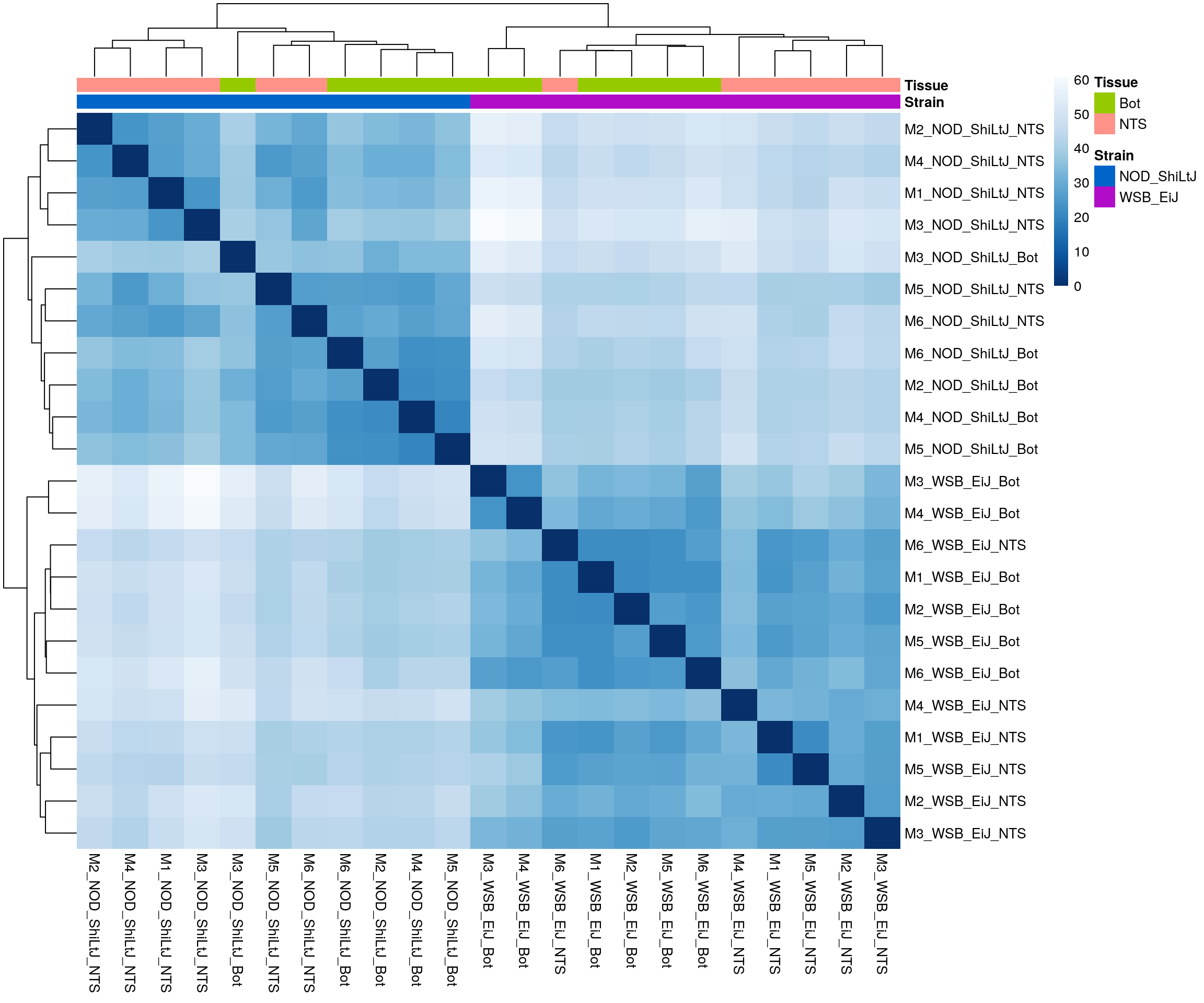
#heatmap on correlation matrix
rld_cor <- cor(assay(rld))
pheatmap(rld_cor,
         annotation_col  = df,
         clustering_distance_rows = "correlation",
         clustering_distance_cols = "correlation",
         annotation_colors = list(Strain = c(NOD_ShiLtJ = "#0064C9",
                                             WSB_EiJ    ="#B10DC9"),
                                  Tissue = c(Bot = "#96ca00",
                                             NTS = "#ff9289")),
         border_color = NA)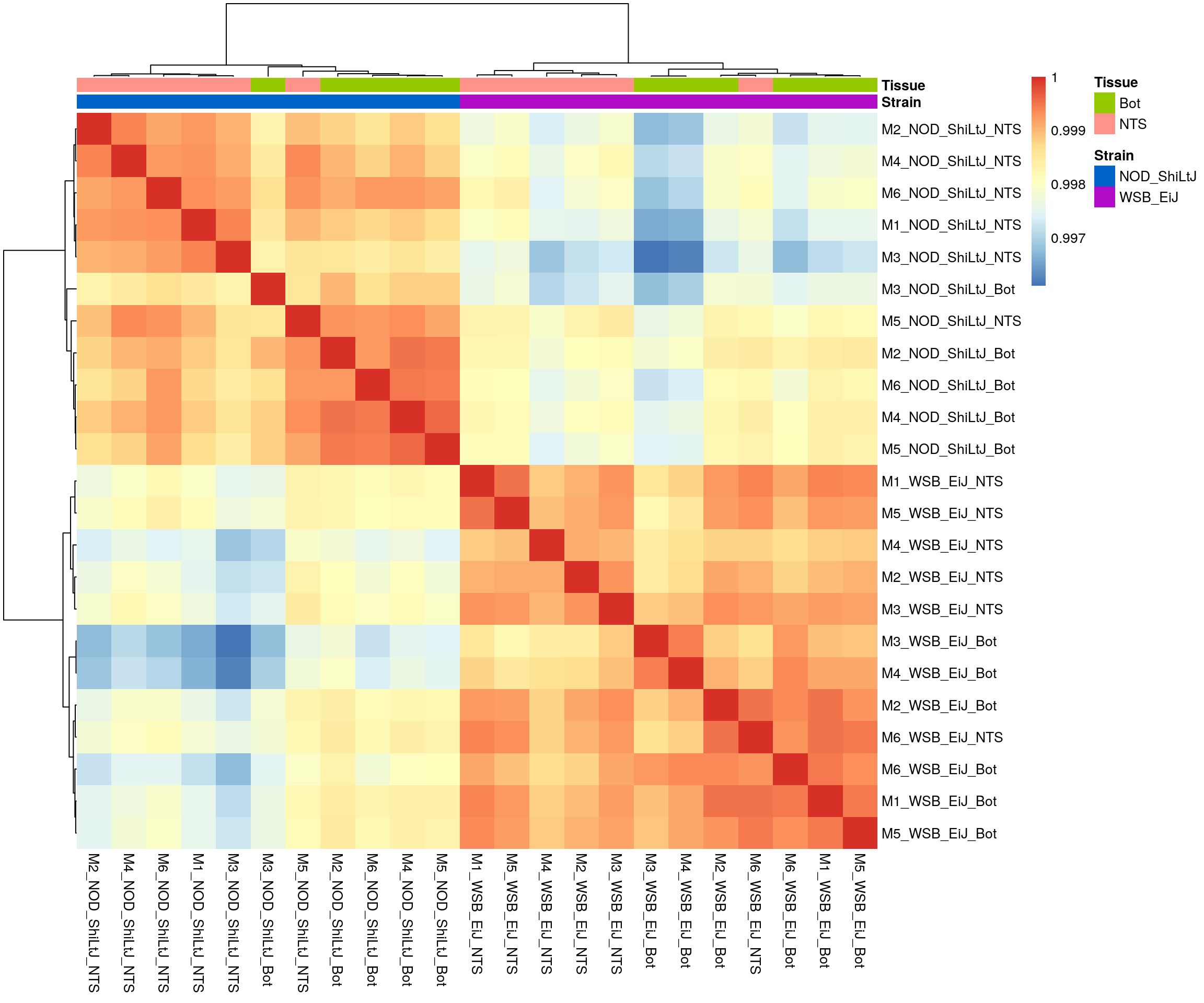
#PCA plot
#Another way to visualize sample-to-sample distances is a principal components analysis (PCA).
pca.plot <- plotPCA(rld, intgroup = c("Strain", "Tissue"), returnData = FALSE)
pca.plot$data$name[!pca.plot$data$name %in% c("M6_WSB_EiJ_NTS", "M5_NOD_ShiLtJ_NTS")] = ""
pca.plot + geom_text(aes(label=name))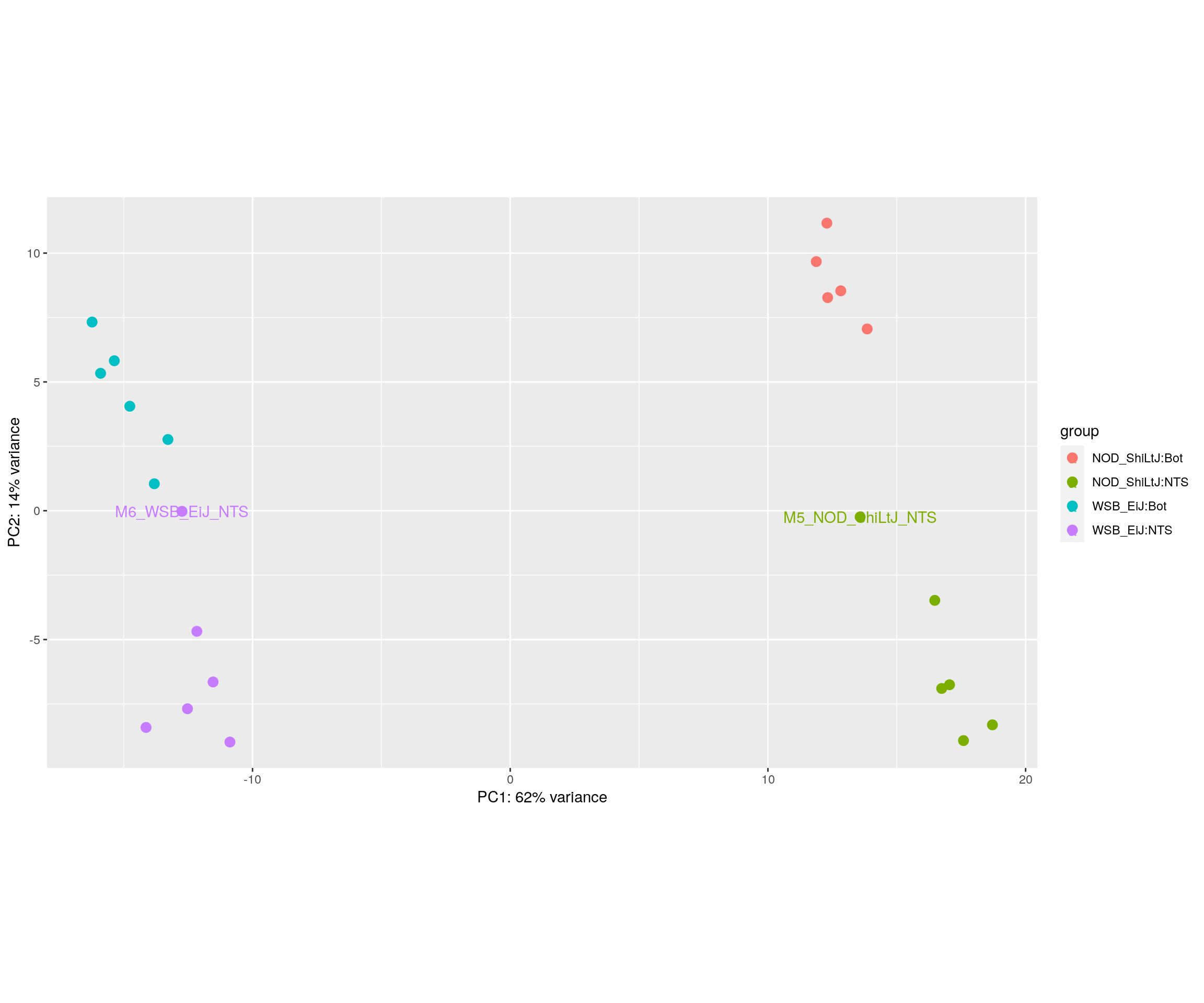
| Version | Author | Date |
|---|---|---|
| f6ccb3e | xhyuo | 2021-07-01 |
Differential expression analysis without interaction term
design(ddsMat)~Strain + Tissue#Running the differential expression pipeline
res <- DESeq(ddsMat)estimating size factorsestimating dispersionsgene-wise dispersion estimatesmean-dispersion relationshipfinal dispersion estimatesfitting model and testingresultsNames(res)[1] "Intercept" "Strain_WSB_EiJ_vs_NOD_ShiLtJ"
[3] "Tissue_NTS_vs_Bot" #comparison for tissue------
#Building the results table
res.tab.tissue <- results(res, name = "Tissue_NTS_vs_Bot", alpha = 0.05)
res.tab.tissuelog2 fold change (MLE): Tissue NTS vs Bot
Wald test p-value: Tissue NTS vs Bot
DataFrame with 27095 rows and 6 columns
baseMean log2FoldChange lfcSE stat pvalue
<numeric> <numeric> <numeric> <numeric> <numeric>
ENSMUSG00000000001 1127.97755 0.0728664 0.0627298 1.161593 0.2454009
ENSMUSG00000000028 55.94968 0.1956631 0.1972510 0.991950 0.3212221
ENSMUSG00000000031 20.36690 0.9934598 0.4043481 2.456942 0.0140125
ENSMUSG00000000037 34.97867 -0.3999197 0.2470309 -1.618905 0.1054676
ENSMUSG00000000049 8.17868 0.1342608 0.5518080 0.243311 0.8077648
... ... ... ... ... ...
ENSMUSG00000108290 0.418612 1.6811417 2.3313686 0.721097 0.47085014
ENSMUSG00000108291 61.786389 -0.2822984 0.1931813 -1.461313 0.14392948
ENSMUSG00000108292 0.899820 -2.3373443 1.9843849 -1.177868 0.23884906
ENSMUSG00000108297 320.366792 -0.2671658 0.0946188 -2.823601 0.00474874
ENSMUSG00000108298 5.447625 -0.0895458 0.6677887 -0.134093 0.89332899
padj
<numeric>
ENSMUSG00000000001 0.626246
ENSMUSG00000000028 0.695761
ENSMUSG00000000031 0.146085
ENSMUSG00000000037 0.431115
ENSMUSG00000000049 0.945468
... ...
ENSMUSG00000108290 NA
ENSMUSG00000108291 0.4999679
ENSMUSG00000108292 NA
ENSMUSG00000108297 0.0758803
ENSMUSG00000108298 0.9724107summary(res.tab.tissue)
out of 27095 with nonzero total read count
adjusted p-value < 0.05
LFC > 0 (up) : 728, 2.7%
LFC < 0 (down) : 399, 1.5%
outliers [1] : 115, 0.42%
low counts [2] : 4130, 15%
(mean count < 3)
[1] see 'cooksCutoff' argument of ?results
[2] see 'independentFiltering' argument of ?resultstable(res.tab.tissue$padj < 0.05)
FALSE TRUE
21723 1127 #We subset the results table to these genes and then sort it by the log2 fold change estimate to get the significant genes with the strongest down-regulation:
resSig.tissue <- subset(res.tab.tissue, padj < 0.05)
head(resSig.tissue[order(resSig.tissue$log2FoldChange), ])log2 fold change (MLE): Tissue NTS vs Bot
Wald test p-value: Tissue NTS vs Bot
DataFrame with 6 rows and 6 columns
baseMean log2FoldChange lfcSE stat pvalue
<numeric> <numeric> <numeric> <numeric> <numeric>
ENSMUSG00000051490 13.66976 -6.61775 1.723765 -3.83913 1.23473e-04
ENSMUSG00000005917 27.02524 -4.22166 0.788465 -5.35427 8.59029e-08
ENSMUSG00000041567 2.98939 -3.27673 1.076240 -3.04461 2.32980e-03
ENSMUSG00000082744 3.10364 -3.27388 0.780042 -4.19706 2.70405e-05
ENSMUSG00000023159 4.68350 -3.18057 0.862083 -3.68941 2.24778e-04
ENSMUSG00000097748 6.88360 -2.95154 0.877669 -3.36293 7.71198e-04
padj
<numeric>
ENSMUSG00000051490 6.34015e-03
ENSMUSG00000005917 1.92439e-05
ENSMUSG00000041567 4.81787e-02
ENSMUSG00000082744 2.00609e-03
ENSMUSG00000023159 9.45890e-03
ENSMUSG00000097748 2.25509e-02# with the strongest up-regulation:
head(resSig.tissue[order(resSig.tissue$log2FoldChange, decreasing = TRUE), ])log2 fold change (MLE): Tissue NTS vs Bot
Wald test p-value: Tissue NTS vs Bot
DataFrame with 6 rows and 6 columns
baseMean log2FoldChange lfcSE stat pvalue
<numeric> <numeric> <numeric> <numeric> <numeric>
ENSMUSG00000000394 26.12756 8.05636 1.569084 5.13444 2.82987e-07
ENSMUSG00000056648 808.28450 8.01199 0.885758 9.04534 1.49198e-19
ENSMUSG00000000690 436.15707 7.52470 0.767824 9.80004 1.12539e-22
ENSMUSG00000043219 51.47675 7.45317 0.904164 8.24316 1.67716e-16
ENSMUSG00000038721 245.43770 6.77881 0.895105 7.57321 3.64127e-14
ENSMUSG00000067220 7.80808 6.35472 1.802334 3.52583 4.22164e-04
padj
<numeric>
ENSMUSG00000000394 4.78982e-05
ENSMUSG00000056648 6.81835e-16
ENSMUSG00000000690 6.42877e-19
ENSMUSG00000043219 3.83232e-13
ENSMUSG00000038721 5.94307e-11
ENSMUSG00000067220 1.51198e-02#comparison for strain------
#Building the results table
res.tab.strain <- results(res, name = "Strain_WSB_EiJ_vs_NOD_ShiLtJ", alpha = 0.05)
res.tab.strainlog2 fold change (MLE): Strain WSB EiJ vs NOD ShiLtJ
Wald test p-value: Strain WSB EiJ vs NOD ShiLtJ
DataFrame with 27095 rows and 6 columns
baseMean log2FoldChange lfcSE stat pvalue
<numeric> <numeric> <numeric> <numeric> <numeric>
ENSMUSG00000000001 1127.97755 -0.1404777 0.062710 -2.240114 0.0250835
ENSMUSG00000000028 55.94968 -0.2304641 0.197026 -1.169711 0.2421172
ENSMUSG00000000031 20.36690 -0.2834524 0.403041 -0.703284 0.4818790
ENSMUSG00000000037 34.97867 -0.0733625 0.247152 -0.296831 0.7665952
ENSMUSG00000000049 8.17868 -0.0669243 0.551505 -0.121348 0.9034151
... ... ... ... ... ...
ENSMUSG00000108290 0.418612 -0.144464 2.3286909 -0.0620364 9.50534e-01
ENSMUSG00000108291 61.786389 0.524922 0.1935960 2.7114324 6.69932e-03
ENSMUSG00000108292 0.899820 0.260944 1.9862984 0.1313719 8.95481e-01
ENSMUSG00000108297 320.366792 0.370040 0.0947347 3.9060644 9.38115e-05
ENSMUSG00000108298 5.447625 1.284852 0.6719124 1.9122315 5.58465e-02
padj
<numeric>
ENSMUSG00000000001 0.0791557
ENSMUSG00000000028 0.4209827
ENSMUSG00000000031 0.6605971
ENSMUSG00000000037 0.8700598
ENSMUSG00000000049 0.9515443
... ...
ENSMUSG00000108290 NA
ENSMUSG00000108291 0.027327987
ENSMUSG00000108292 0.946717455
ENSMUSG00000108297 0.000703195
ENSMUSG00000108298 0.146199788summary(res.tab.strain)
out of 27095 with nonzero total read count
adjusted p-value < 0.05
LFC > 0 (up) : 3375, 12%
LFC < 0 (down) : 3767, 14%
outliers [1] : 115, 0.42%
low counts [2] : 1542, 5.7%
(mean count < 1)
[1] see 'cooksCutoff' argument of ?results
[2] see 'independentFiltering' argument of ?resultstable(res.tab.strain$padj < 0.05)
FALSE TRUE
18296 7142 #We subset the results table to these genes and then sort it by the log2 fold change estimate to get the significant genes with the strongest down-regulation:
resSig.strain <- subset(res.tab.strain, padj < 0.05)
head(resSig.strain[order(resSig.strain$log2FoldChange), ])log2 fold change (MLE): Strain WSB EiJ vs NOD ShiLtJ
Wald test p-value: Strain WSB EiJ vs NOD ShiLtJ
DataFrame with 6 rows and 6 columns
baseMean log2FoldChange lfcSE stat pvalue
<numeric> <numeric> <numeric> <numeric> <numeric>
ENSMUSG00000092365 362.6730 -11.97377 0.595477 -20.1079 6.29608e-90
ENSMUSG00000053038 463.7134 -11.86525 0.604382 -19.6321 8.23116e-86
ENSMUSG00000066553 173.8310 -10.67636 0.595832 -17.9184 8.47015e-72
ENSMUSG00000079018 258.6623 -10.29985 0.598334 -17.2142 2.07760e-66
ENSMUSG00000101878 99.9184 -10.08768 0.607398 -16.6080 6.09743e-62
ENSMUSG00000094891 65.4140 -9.51953 0.617116 -15.4258 1.09730e-53
padj
<numeric>
ENSMUSG00000092365 2.22444e-87
ENSMUSG00000053038 2.55347e-83
ENSMUSG00000066553 2.11239e-69
ENSMUSG00000079018 4.55604e-64
ENSMUSG00000101878 1.23100e-59
ENSMUSG00000094891 1.92505e-51# with the strongest up-regulation:
head(resSig.strain[order(resSig.strain$log2FoldChange, decreasing = TRUE), ])log2 fold change (MLE): Strain WSB EiJ vs NOD ShiLtJ
Wald test p-value: Strain WSB EiJ vs NOD ShiLtJ
DataFrame with 6 rows and 6 columns
baseMean log2FoldChange lfcSE stat pvalue
<numeric> <numeric> <numeric> <numeric> <numeric>
ENSMUSG00000094306 2237.4111 13.76796 0.623644 22.0766 5.30147e-108
ENSMUSG00000096039 109.3540 10.18498 0.628856 16.1960 5.37734e-59
ENSMUSG00000103706 105.4107 9.88015 0.629553 15.6939 1.66467e-55
ENSMUSG00000094518 138.1547 9.74873 0.640311 15.2250 2.41352e-52
ENSMUSG00000021908 1579.3642 9.26278 0.215687 42.9454 0.00000e+00
ENSMUSG00000083773 42.0801 8.82378 0.640299 13.7807 3.32951e-43
padj
<numeric>
ENSMUSG00000094306 2.10717e-105
ENSMUSG00000096039 1.05222e-56
ENSMUSG00000103706 3.02471e-53
ENSMUSG00000094518 4.03915e-50
ENSMUSG00000021908 0.00000e+00
ENSMUSG00000083773 4.48127e-41Visualization
#Visualization for tissue result------
#Volcano plot
## Obtain logical vector regarding whether padj values are less than 0.05
threshold_OE <- (res.tab.tissue$padj < 0.05 & abs(res.tab.tissue$log2FoldChange) >= 1)
## Determine the number of TRUE values
length(which(threshold_OE))[1] 262## Add logical vector as a column (threshold) to the res.tab.tissue
res.tab.tissue$threshold <- threshold_OE
## Sort by ordered padj
res.tab.tissue_ordered <- res.tab.tissue %>%
data.frame() %>%
rownames_to_column(var="ENSEMBL") %>%
arrange(padj) %>%
mutate(genelabels = "") %>%
as_tibble() %>%
left_join(genes)Joining, by = "ENSEMBL"## Create a column to indicate which genes to label
res.tab.tissue_ordered$genelabels[1:10] <- res.tab.tissue_ordered$SYMBOL[1:10]
#display res.tab.tissue_ordered
DT::datatable(res.tab.tissue_ordered[res.tab.tissue_ordered$padj < 0.05,],
filter = list(position = 'top', clear = FALSE),
options = list(pageLength = 40, scrollY = "300px", scrollX = "40px"),
caption = htmltools::tags$caption(style = 'caption-side: top; text-align: left; color:black; font-size:200% ;','DEG analysis tissue results (fdr < 0.05)'))#Volcano plot
volcano.plot.tissue <- ggplot(res.tab.tissue_ordered) +
geom_point(aes(x = log2FoldChange, y = -log10(padj), colour = threshold)) +
scale_color_manual(values=c("blue", "red")) +
geom_text_repel(aes(x = log2FoldChange, y = -log10(padj),
label = genelabels,
size = 3.5)) +
ggtitle("DEG for Tissue NTS vs Bot") +
xlab("log2 fold change") +
ylab("-log10 adjusted p-value") +
theme(legend.position = "none",
plot.title = element_text(size = rel(1.5), hjust = 0.5),
axis.title = element_text(size = rel(1.25)))
print(volcano.plot.tissue)Warning: Removed 4245 rows containing missing values (geom_point).Warning: Removed 4245 rows containing missing values (geom_text_repel).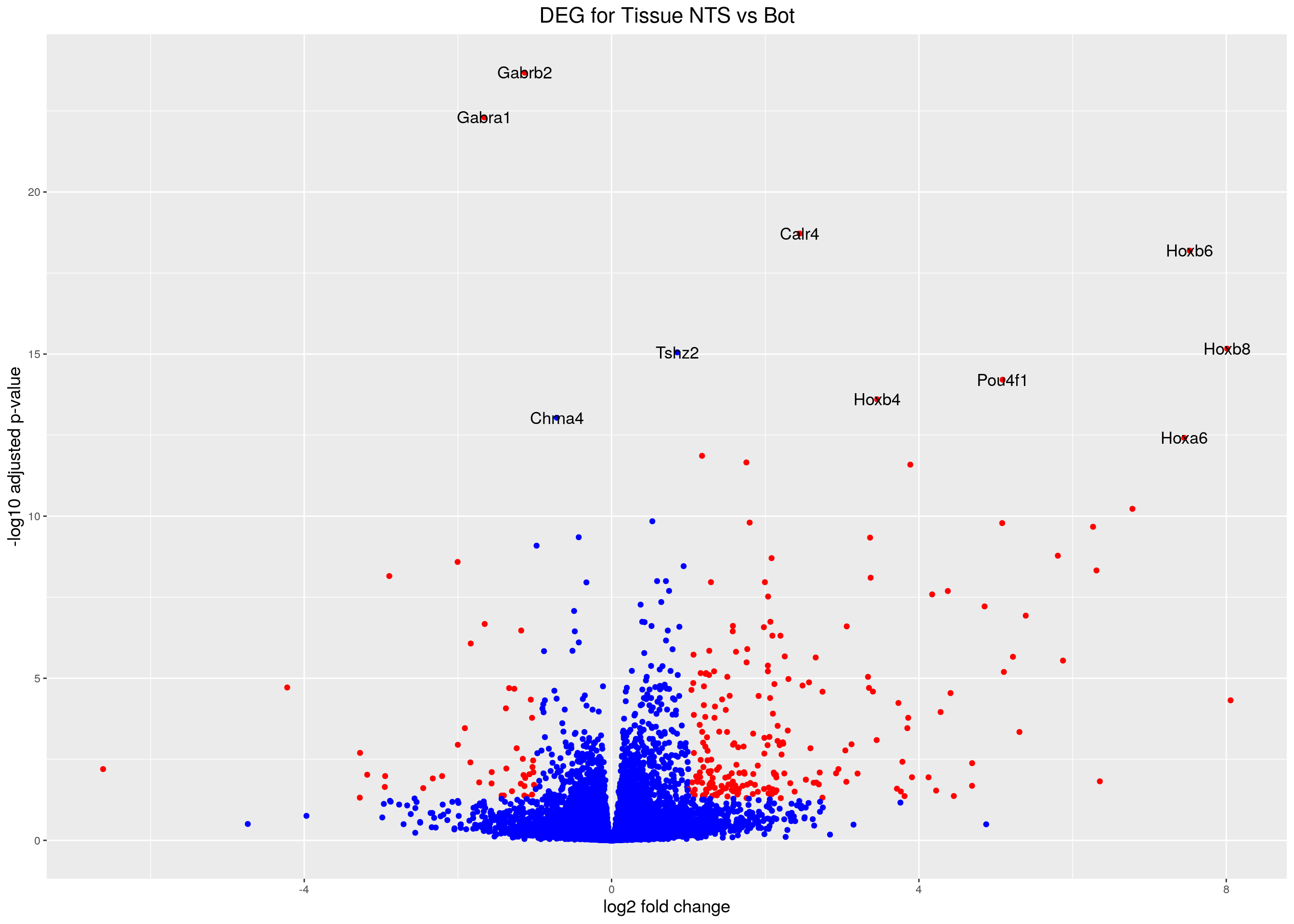
#heatmap
# Extract normalized expression for significant genes fdr < 0.05 & abs(log2FoldChange) >= 1)
normalized_counts_sig.tissue <- normalized_counts %>%
filter(gene %in% rownames(subset(resSig.tissue, padj < 0.05 & abs(log2FoldChange) >= 1)))
### Set a color palette
heat_colors <- brewer.pal(6, "YlOrRd")
#annotation
df <- as.data.frame(colData(ddsMat)[,c("Strain","Tissue")])
### Run pheatmap using the metadata data frame for the annotation
pheatmap(as.matrix(normalized_counts_sig.tissue[,-1]),
color = heat_colors,
cluster_rows = T,
show_rownames = F,
annotation_col = df,
annotation_colors = list(Strain = c(NOD_ShiLtJ = "#0064C9",
WSB_EiJ ="#B10DC9"),
Tissue = c(Bot = "#96ca00",
NTS = "#ff9289")),
border_color = NA,
fontsize = 10,
scale = "row",
fontsize_row = 10,
height = 20,
main = "Heatmap of the top DEGs in Tissue NTS vs Bot (fdr < 0.05 & abs(log2FoldChange) >= 1)")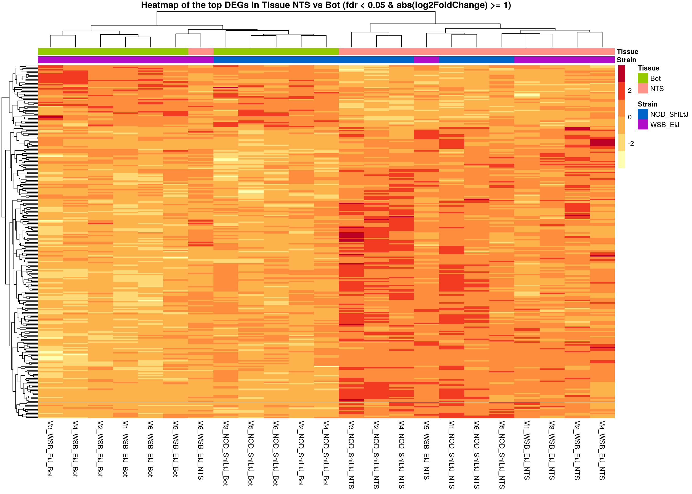
#Visualization for strain result------
#Volcano plot
## Obtain logical vector regarding whether padj values are less than 0.05
threshold_OE <- (res.tab.strain$padj < 0.05 & abs(res.tab.strain$log2FoldChange) >= 1)
## Determine the number of TRUE values
length(which(threshold_OE))[1] 1748## Add logical vector as a column (threshold) to the res.tab.strain
res.tab.strain$threshold <- threshold_OE
## Sort by ordered padj
res.tab.strain_ordered <- res.tab.strain %>%
data.frame() %>%
rownames_to_column(var="ENSEMBL") %>%
arrange(padj) %>%
mutate(genelabels = "") %>%
as_tibble() %>%
left_join(genes)Joining, by = "ENSEMBL"## Create a column to indicate which genes to label
res.tab.strain_ordered$genelabels[1:10] <- res.tab.strain_ordered$SYMBOL[1:10]
#display res.tab.strain_ordered
DT::datatable(res.tab.strain_ordered[res.tab.strain_ordered$padj < 0.05,],
filter = list(position = 'top', clear = FALSE),
options = list(pageLength = 40, scrollY = "300px", scrollX = "40px"),
caption = htmltools::tags$caption(style = 'caption-side: top; text-align: left; color:black; font-size:200% ;','DEG analysis strain results (fdr < 0.05)'))Warning in instance$preRenderHook(instance): It seems your data is too big
for client-side DataTables. You may consider server-side processing: https://
rstudio.github.io/DT/server.html#Volcano plot
volcano.plot.strain <- ggplot(res.tab.strain_ordered) +
geom_point(aes(x = log2FoldChange, y = -log10(padj), colour = threshold)) +
scale_color_manual(values=c("blue", "red")) +
geom_text_repel(aes(x = log2FoldChange, y = -log10(padj),
label = genelabels,
size = 3.5)) +
ggtitle("DEG for Strain WSB_EiJ vs NOD_ShiLtJ") +
xlab("log2 fold change") +
ylab("-log10 adjusted p-value") +
theme(legend.position = "none",
plot.title = element_text(size = rel(1.5), hjust = 0.5),
axis.title = element_text(size = rel(1.25)))
print(volcano.plot.strain)Warning: Removed 1657 rows containing missing values (geom_point).Warning: Removed 1659 rows containing missing values (geom_text_repel).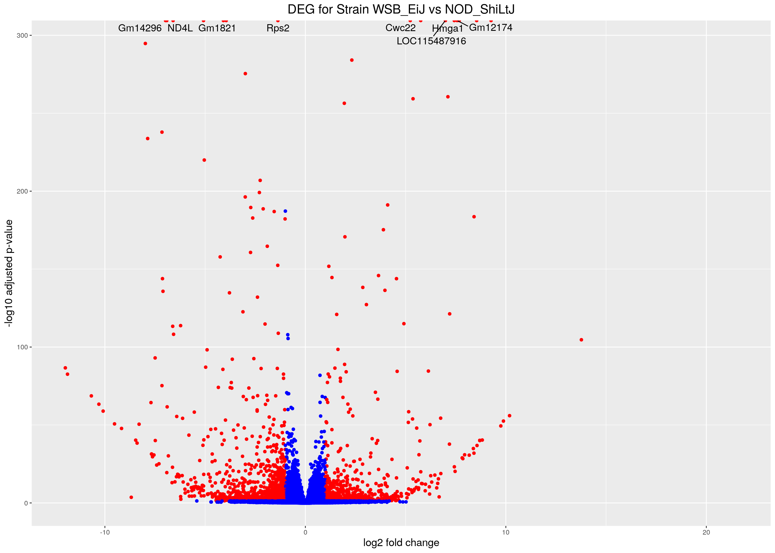
#heatmap
# Extract normalized expression for significant genes fdr < 0.05 & abs(log2FoldChange) >= 1)
normalized_counts_sig.strain <- normalized_counts %>%
filter(gene %in% rownames(subset(resSig.strain, padj < 0.05 & abs(log2FoldChange) >= 1)))
### Set a color palette
heat_colors <- brewer.pal(6, "YlOrRd")
#annotation
df <- as.data.frame(colData(ddsMat)[,c("Strain","Tissue")])
### Run pheatmap using the metadata data frame for the annotation
pheatmap(as.matrix(normalized_counts_sig.strain[,-1]),
color = heat_colors,
cluster_rows = T,
show_rownames = F,
annotation_col = df,
annotation_colors = list(Strain = c(NOD_ShiLtJ = "#0064C9",
WSB_EiJ ="#B10DC9"),
Tissue = c(Bot = "#96ca00",
NTS = "#ff9289")),
border_color = NA,
fontsize = 10,
scale = "row",
fontsize_row = 10,
height = 20,
main = "Heatmap of the top DEGs in Strain WSB_EiJ vs NOD_ShiLtJ(fdr < 0.05 & abs(log2FoldChange) >= 1)")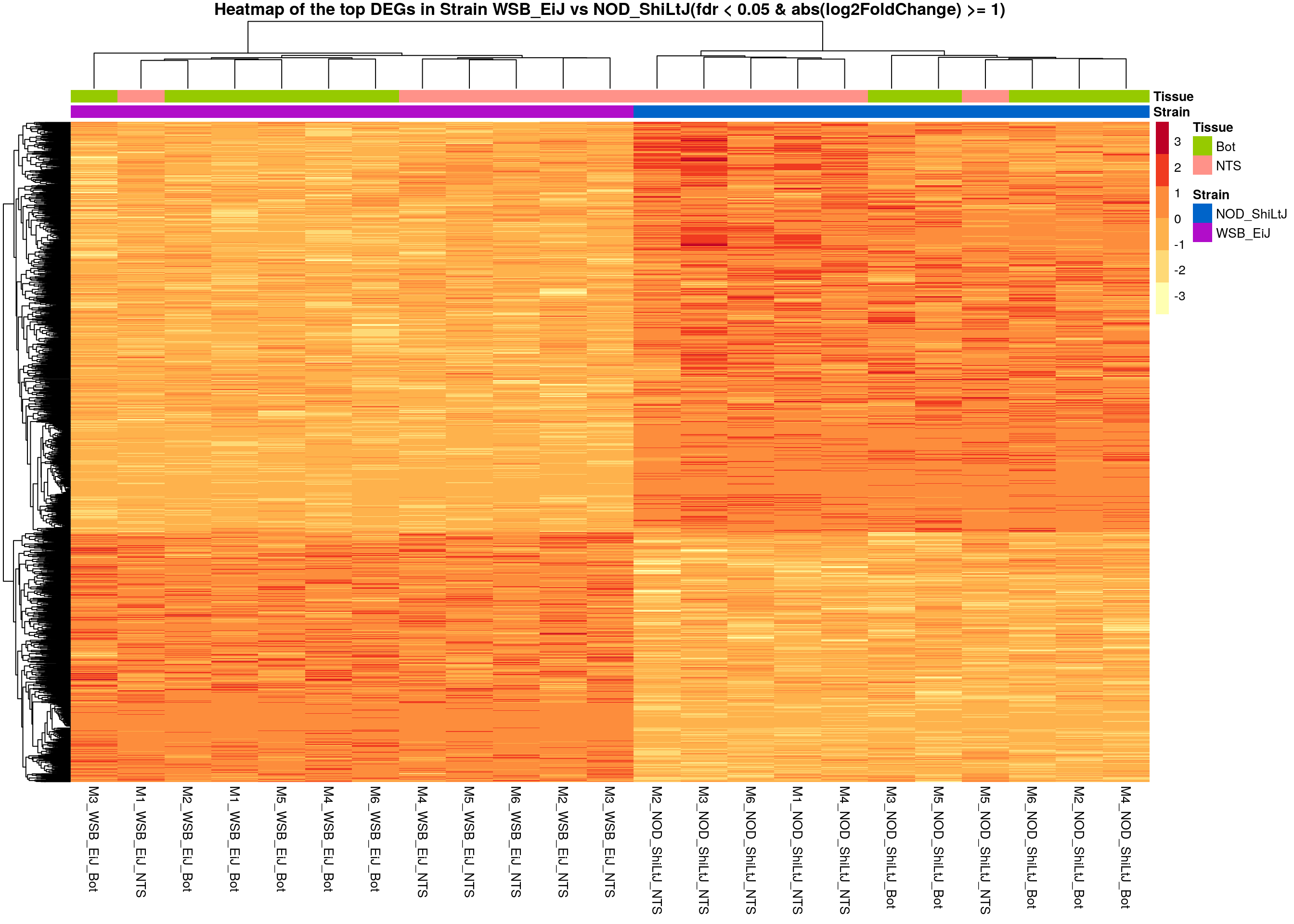
#heatmap on both strain and tissue top DEGs-----
normalized_counts_sig.strain.tissue <- normalized_counts %>%
filter(gene %in% unique(rownames(subset(resSig.tissue, padj < 0.05 & abs(log2FoldChange) >= 1)),
rownames(subset(resSig.strain, padj < 0.05 & abs(log2FoldChange) >= 1))))
### Set a color palette
heat_colors <- brewer.pal(6, "YlOrRd")
#annotation
df <- as.data.frame(colData(ddsMat)[,c("Strain","Tissue")])
### Run pheatmap using the metadata data frame for the annotation
pheatmap(as.matrix(normalized_counts_sig.strain.tissue[,-1]),
color = heat_colors,
cluster_rows = T,
show_rownames = F,
annotation_col = df,
annotation_colors = list(Strain = c(NOD_ShiLtJ = "#0064C9",
WSB_EiJ ="#B10DC9"),
Tissue = c(Bot = "#96ca00",
NTS = "#ff9289")),
border_color = NA,
fontsize = 10,
scale = "row",
fontsize_row = 10,
height = 20,
main = "Heatmap of the top DEGs in Both Strain and Tissue (fdr < 0.05 & abs(log2FoldChange) >= 1)")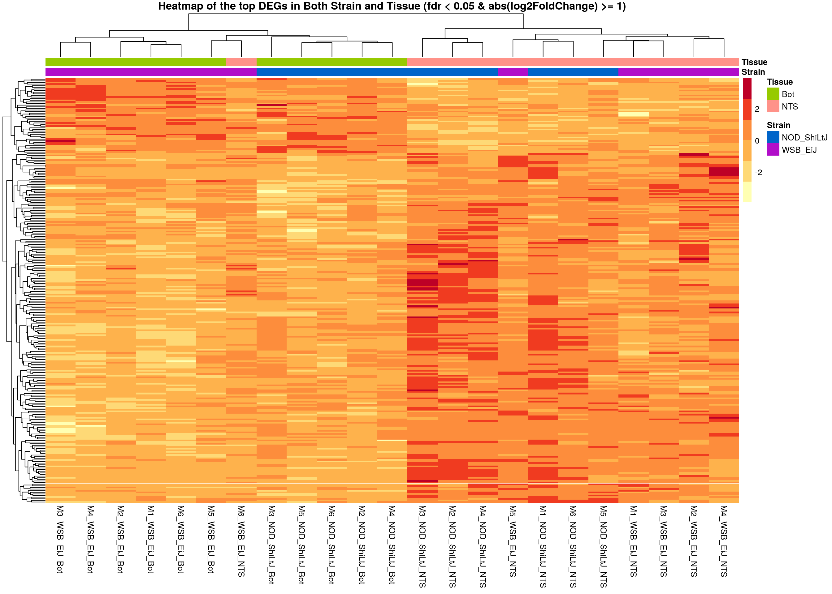
#logFC heatmap on both strain and tissue top DEGs-----
restop.tab.strain.tissue <- full_join(res.tab.strain_ordered,
res.tab.tissue_ordered,
by = c("ENSEMBL", "SYMBOL")) %>%
filter((ENSEMBL %in% res.tab.strain_ordered$ENSEMBL[1:30]) | (ENSEMBL %in% res.tab.tissue_ordered$ENSEMBL[1:30]))
restop.tab.strain.tissue.mat <- as.matrix(restop.tab.strain.tissue[, c("log2FoldChange.x", "log2FoldChange.y")])
rownames(restop.tab.strain.tissue.mat) <-
ifelse(is.na(restop.tab.strain.tissue$SYMBOL),
restop.tab.strain.tissue$ENSEMBL,
paste0(restop.tab.strain.tissue$SYMBOL,":", restop.tab.strain.tissue$ENSEMBL))
colnames(restop.tab.strain.tissue.mat) <- c("strain", "tissue")
#heatmap
### Run pheatmap using the metadata data frame for the annotation
pheatmap(restop.tab.strain.tissue.mat,
color = colorpanel(1000, "blue", "white", "red"),
cluster_rows = T,
show_rownames = T,
border_color = NA,
fontsize = 10,
fontsize_row = 8,
height = 25,
main = "Heatmap of log2FoldChange for the top 30 DEGs in Strain or Tissue")
Enrichment
#enrichment analysis
dbs <- c("WikiPathways_2019_Mouse",
"GO_Biological_Process_2021",
"GO_Cellular_Component_2021",
"GO_Molecular_Function_2021",
"KEGG_2019_Mouse",
"Mouse_Gene_Atlas",
"MGI_Mammalian_Phenotype_Level_4_2019")
#tissue results------
resSig.tissue.tab <- resSig.tissue %>%
data.frame() %>%
rownames_to_column(var="ENSEMBL") %>%
as_tibble() %>%
left_join(genes)Joining, by = "ENSEMBL"#up-regulated tissue genes---------------------------
up.genes <- resSig.tissue.tab %>%
filter(log2FoldChange > 0) %>%
pull(SYMBOL)
#up-regulated genes enrichment
up.genes.enriched <- enrichr(as.character(na.omit(up.genes)), dbs)Uploading data to Enrichr... Done.
Querying WikiPathways_2019_Mouse... Done.
Querying GO_Biological_Process_2021... Done.
Querying GO_Cellular_Component_2021... Done.
Querying GO_Molecular_Function_2021... Done.
Querying KEGG_2019_Mouse... Done.
Querying Mouse_Gene_Atlas... Done.
Querying MGI_Mammalian_Phenotype_Level_4_2019... Done.
Parsing results... Done.for (j in 1:length(up.genes.enriched)){
up.genes.enriched[[j]] <- cbind(data.frame(Library = names(up.genes.enriched)[j]),up.genes.enriched[[j]])
}
up.genes.enriched <- do.call(rbind.data.frame, up.genes.enriched) %>%
filter(Adjusted.P.value <= 0.05) %>%
mutate(logpvalue = -log10(P.value)) %>%
arrange(desc(logpvalue))
#display up.genes.enriched
DT::datatable(up.genes.enriched,filter = list(position = 'top', clear = FALSE),
options = list(pageLength = 40, scrollY = "300px", scrollX = "40px"))#barpot
up.genes.enriched.plot <- up.genes.enriched %>%
filter(Adjusted.P.value <= 0.001) %>%
mutate(Term = fct_reorder(Term, -logpvalue)) %>%
ggplot(data = ., aes(x = Term, y = logpvalue, fill = Library, label = Overlap)) +
geom_bar(stat = "identity") +
geom_text(position = position_dodge(width = 0.9),
hjust = 0) +
theme_bw() +
ylab("-log(p.value)") +
xlab("") +
ggtitle("Enrichment of up-regulated tissue genes \n(Adjusted.P.value <= 0.001)") +
theme(plot.background = element_blank() ,
panel.border = element_blank(),
panel.background = element_blank(),
#legend.position = "none",
plot.title = element_text(hjust = 0),
panel.grid.major = element_blank(),
panel.grid.minor = element_blank()) +
theme(axis.line = element_line(color = 'black')) +
theme(axis.title.x = element_text(size = 12, vjust=-0.5)) +
theme(axis.title.y = element_text(size = 12, vjust= 1.0)) +
theme(axis.text = element_text(size = 12)) +
theme(plot.title = element_text(size = 12)) +
coord_flip()
up.genes.enriched.plot
#down-regulated tissue genes---------------------------
down.genes <- resSig.tissue.tab %>%
filter(log2FoldChange < 0) %>%
pull(SYMBOL)
#down-regulated genes enrichment
down.genes.enriched <- enrichr(as.character(na.omit(down.genes)), dbs)Uploading data to Enrichr... Done.
Querying WikiPathways_2019_Mouse... Done.
Querying GO_Biological_Process_2021... Done.
Querying GO_Cellular_Component_2021... Done.
Querying GO_Molecular_Function_2021... Done.
Querying KEGG_2019_Mouse... Done.
Querying Mouse_Gene_Atlas... Done.
Querying MGI_Mammalian_Phenotype_Level_4_2019... Done.
Parsing results... Done.for (j in 1:length(down.genes.enriched)){
down.genes.enriched[[j]] <- cbind(data.frame(Library = names(down.genes.enriched)[j]),down.genes.enriched[[j]])
}
down.genes.enriched <- do.call(rbind.data.frame, down.genes.enriched) %>%
filter(Adjusted.P.value <= 0.05) %>%
mutate(logpvalue = -log10(P.value)) %>%
arrange(desc(logpvalue))
#display down.genes.enriched
DT::datatable(down.genes.enriched,filter = list(position = 'top', clear = FALSE),
options = list(pageLength = 40, scrollY = "300px", scrollX = "40px"))#barpot
down.genes.enriched.plot <- down.genes.enriched %>%
filter(Adjusted.P.value <= 0.01) %>%
mutate(Term = fct_reorder(Term, -logpvalue)) %>%
ggplot(data = ., aes(x = Term, y = logpvalue, fill = Library, label = Overlap)) +
geom_bar(stat = "identity") +
geom_text(position = position_dodge(width = 0.9),
hjust = 0) +
theme_bw() +
ylab("-log(p.value)") +
xlab("") +
ggtitle("Enrichment of down-regulated tissue genes \n(Adjusted.P.value <= 0.01)") +
theme(plot.background = element_blank() ,
panel.border = element_blank(),
panel.background = element_blank(),
#legend.position = "none",
plot.title = element_text(hjust = 0),
panel.grid.major = element_blank(),
panel.grid.minor = element_blank()) +
theme(axis.line = element_line(color = 'black')) +
theme(axis.title.x = element_text(size = 12, vjust=-0.5)) +
theme(axis.title.y = element_text(size = 12, vjust= 1.0)) +
theme(axis.text = element_text(size = 12)) +
theme(plot.title = element_text(size = 12)) +
coord_flip()
down.genes.enriched.plot
#strain results------
resSig.strain.tab <- resSig.strain %>%
data.frame() %>%
rownames_to_column(var="ENSEMBL") %>%
as_tibble() %>%
left_join(genes)Joining, by = "ENSEMBL"#up-regulated strain genes---------------------------
up.genes <- resSig.strain.tab %>%
filter(log2FoldChange > 0) %>%
pull(SYMBOL)
#up-regulated genes enrichment
up.genes.enriched <- enrichr(as.character(na.omit(up.genes)), dbs)Uploading data to Enrichr... Done.
Querying WikiPathways_2019_Mouse... Done.
Querying GO_Biological_Process_2021... Done.
Querying GO_Cellular_Component_2021... Done.
Querying GO_Molecular_Function_2021... Done.
Querying KEGG_2019_Mouse... Done.
Querying Mouse_Gene_Atlas... Done.
Querying MGI_Mammalian_Phenotype_Level_4_2019... Done.
Parsing results... Done.for (j in 1:length(up.genes.enriched)){
up.genes.enriched[[j]] <- cbind(data.frame(Library = names(up.genes.enriched)[j]),up.genes.enriched[[j]])
}
up.genes.enriched <- do.call(rbind.data.frame, up.genes.enriched) %>%
filter(Adjusted.P.value <= 0.05) %>%
mutate(logpvalue = -log10(P.value)) %>%
arrange(desc(logpvalue))
#display up.genes.enriched
DT::datatable(up.genes.enriched,filter = list(position = 'top', clear = FALSE),
options = list(pageLength = 40, scrollY = "300px", scrollX = "40px"))#barpot
up.genes.enriched.plot <- up.genes.enriched %>%
filter(Adjusted.P.value <= 0.001) %>%
mutate(Term = fct_reorder(Term, -logpvalue)) %>%
ggplot(data = ., aes(x = Term, y = logpvalue, fill = Library, label = Overlap)) +
geom_bar(stat = "identity") +
geom_text(position = position_dodge(width = 0.9),
hjust = 0) +
theme_bw() +
ylab("-log(p.value)") +
xlab("") +
ggtitle("Enrichment of up-regulated strain genes \n(Adjusted.P.value <= 0.001)") +
theme(plot.background = element_blank() ,
panel.border = element_blank(),
panel.background = element_blank(),
#legend.position = "none",
plot.title = element_text(hjust = 0),
panel.grid.major = element_blank(),
panel.grid.minor = element_blank()) +
theme(axis.line = element_line(color = 'black')) +
theme(axis.title.x = element_text(size = 12, vjust=-0.5)) +
theme(axis.title.y = element_text(size = 12, vjust= 1.0)) +
theme(axis.text = element_text(size = 12)) +
theme(plot.title = element_text(size = 12)) +
coord_flip()
up.genes.enriched.plot
#down-regulated strain genes---------------------------
down.genes <- resSig.strain.tab %>%
filter(log2FoldChange < 0) %>%
pull(SYMBOL)
#down-regulated genes enrichment
down.genes.enriched <- enrichr(as.character(na.omit(down.genes)), dbs)Uploading data to Enrichr... Done.
Querying WikiPathways_2019_Mouse... Done.
Querying GO_Biological_Process_2021... Done.
Querying GO_Cellular_Component_2021... Done.
Querying GO_Molecular_Function_2021... Done.
Querying KEGG_2019_Mouse... Done.
Querying Mouse_Gene_Atlas... Done.
Querying MGI_Mammalian_Phenotype_Level_4_2019... Done.
Parsing results... Done.for (j in 1:length(down.genes.enriched)){
down.genes.enriched[[j]] <- cbind(data.frame(Library = names(down.genes.enriched)[j]),down.genes.enriched[[j]])
}
down.genes.enriched <- do.call(rbind.data.frame, down.genes.enriched) %>%
filter(Adjusted.P.value <= 0.05) %>%
mutate(logpvalue = -log10(P.value)) %>%
arrange(desc(logpvalue))
#display down.genes.enriched
DT::datatable(down.genes.enriched,filter = list(position = 'top', clear = FALSE),
options = list(pageLength = 40, scrollY = "300px", scrollX = "40px"))#barpot
down.genes.enriched.plot <- down.genes.enriched %>%
filter(Adjusted.P.value <= 0.001) %>%
mutate(Term = fct_reorder(Term, -logpvalue)) %>%
ggplot(data = ., aes(x = Term, y = logpvalue, fill = Library, label = Overlap)) +
geom_bar(stat = "identity") +
geom_text(position = position_dodge(width = 0.9),
hjust = 0) +
theme_bw() +
ylab("-log(p.value)") +
xlab("") +
ggtitle("Enrichment of down-regulated strain genes \n(Adjusted.P.value <= 0.001)") +
theme(plot.background = element_blank() ,
panel.border = element_blank(),
panel.background = element_blank(),
#legend.position = "none",
plot.title = element_text(hjust = 0),
panel.grid.major = element_blank(),
panel.grid.minor = element_blank()) +
theme(axis.line = element_line(color = 'black')) +
theme(axis.title.x = element_text(size = 12, vjust=-0.5)) +
theme(axis.title.y = element_text(size = 12, vjust= 1.0)) +
theme(axis.text = element_text(size = 12)) +
theme(plot.title = element_text(size = 12)) +
coord_flip()
down.genes.enriched.plot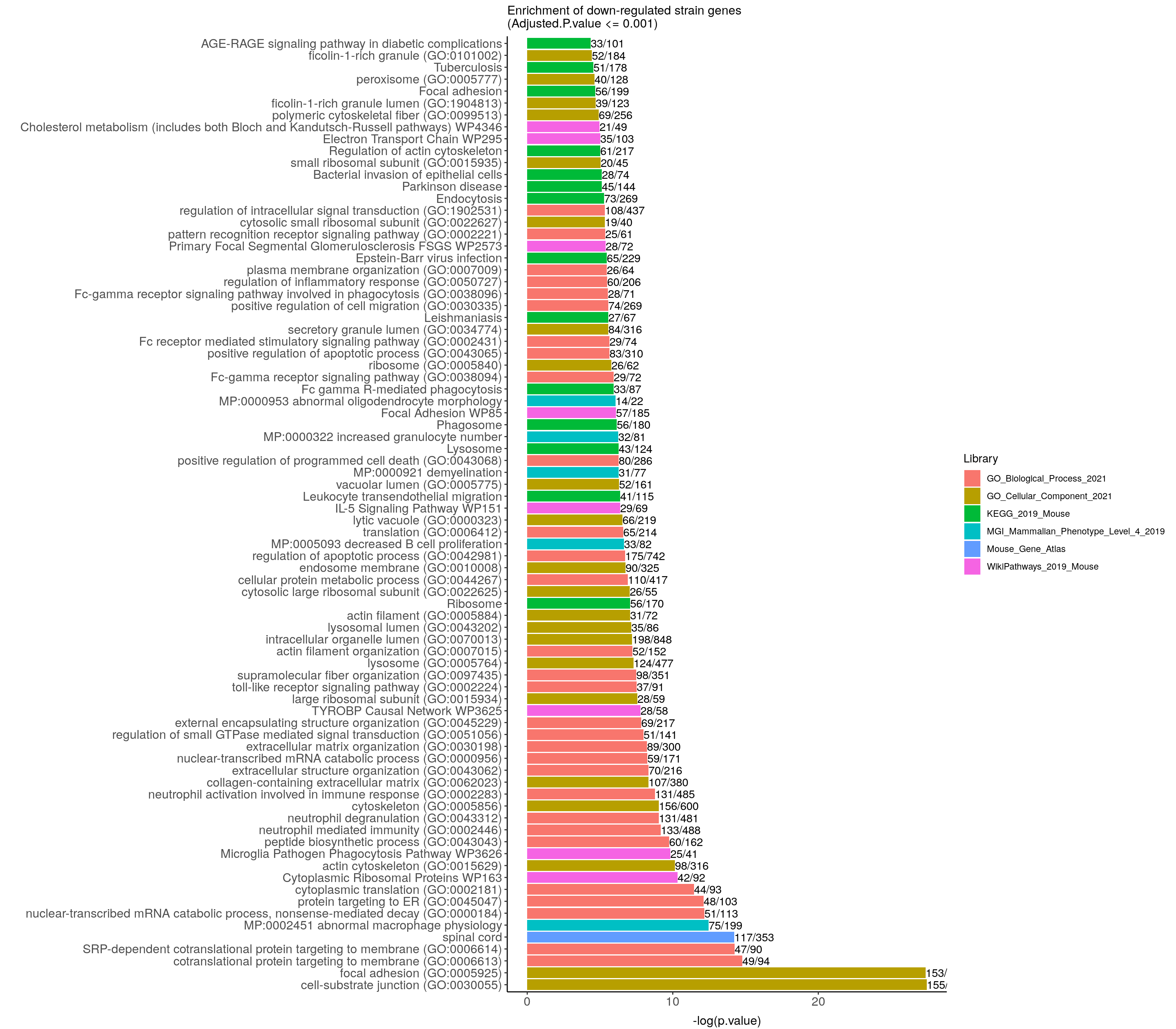
Differential expression analysis with interaction term
design(ddsMat) <- ~Tissue + Strain + Tissue:Strain
#Running the differential expression pipeline
res <- DESeq(ddsMat)
estimating size factorsestimating dispersionsgene-wise dispersion estimatesmean-dispersion relationshipfinal dispersion estimatesfitting model and testingresultsNames(res)[1] "Intercept" "Tissue_NTS_vs_Bot"
[3] "Strain_WSB_EiJ_vs_NOD_ShiLtJ" "TissueNTS.StrainWSB_EiJ" The effect of Strain in Bot
#in Bot, WSB_EiJ compared with NOD_ShiLtJ
#Building the results table
res.tab.strain.in.Bot <- results(res, contrast=c("Strain","WSB_EiJ","NOD_ShiLtJ"), alpha = 0.05)
res.tab.strain.in.Bot
log2 fold change (MLE): Strain WSB_EiJ vs NOD_ShiLtJ
Wald test p-value: Strain WSB EiJ vs NOD ShiLtJ
DataFrame with 27095 rows and 6 columns
baseMean log2FoldChange lfcSE stat pvalue
<numeric> <numeric> <numeric> <numeric> <numeric>
ENSMUSG00000000001 1127.97755 -0.1560307 0.092379 -1.689027 0.0912142
ENSMUSG00000000028 55.94968 -0.0412122 0.288081 -0.143058 0.8862445
ENSMUSG00000000031 20.36690 -0.1008559 0.608333 -0.165791 0.8683218
ENSMUSG00000000037 34.97867 0.4156699 0.333511 1.246347 0.2126371
ENSMUSG00000000049 8.17868 -0.1950056 0.817286 -0.238601 0.8114147
... ... ... ... ... ...
ENSMUSG00000108290 0.418612 0.590142 3.604241 0.163735 0.86993940
ENSMUSG00000108291 61.786389 0.309922 0.276883 1.119325 0.26300163
ENSMUSG00000108292 0.899820 2.234458 2.971549 0.751950 0.45208091
ENSMUSG00000108297 320.366792 0.389602 0.138920 2.804503 0.00503942
ENSMUSG00000108298 5.447625 1.400847 0.997120 1.404893 0.16005311
padj
<numeric>
ENSMUSG00000000001 0.238374
ENSMUSG00000000028 0.947939
ENSMUSG00000000031 0.938453
ENSMUSG00000000037 0.418209
ENSMUSG00000000049 0.909073
... ...
ENSMUSG00000108290 NA
ENSMUSG00000108291 0.477847
ENSMUSG00000108292 NA
ENSMUSG00000108297 0.028144
ENSMUSG00000108298 0.347892summary(res.tab.strain.in.Bot)
out of 27095 with nonzero total read count
adjusted p-value < 0.05
LFC > 0 (up)       : 2393, 8.8%
LFC < 0 (down)     : 2686, 9.9%
outliers [1]       : 42, 0.16%
low counts [2]     : 3139, 12%
(mean count < 2)
[1] see 'cooksCutoff' argument of ?results
[2] see 'independentFiltering' argument of ?results
table(res.tab.strain.in.Bot$padj < 0.05)
FALSE  TRUE
18835  5079
#We subset the results table to these genes and then sort it by the log2 fold change estimate to get the significant genes with the strongest down-regulation:
resSig.strain.in.Bot <- subset(res.tab.strain.in.Bot, padj < 0.05)
head(resSig.strain.in.Bot[order(resSig.strain.in.Bot$log2FoldChange), ])log2 fold change (MLE): Strain WSB_EiJ vs NOD_ShiLtJ
Wald test p-value: Strain WSB EiJ vs NOD ShiLtJ
DataFrame with 6 rows and 6 columns
baseMean log2FoldChange lfcSE stat pvalue
<numeric> <numeric> <numeric> <numeric> <numeric>
ENSMUSG00000053038 463.7134 -12.01728 0.855816 -14.0419 8.63709e-45
ENSMUSG00000092365 362.6730 -11.86570 0.842517 -14.0836 4.78849e-45
ENSMUSG00000066553 173.8310 -10.83494 0.842992 -12.8530 8.27859e-38
ENSMUSG00000079018 258.6623 -10.11674 0.825586 -12.2540 1.59889e-34
ENSMUSG00000101878 99.9184 -9.84555 0.860381 -11.4433 2.54179e-30
ENSMUSG00000094891 65.4140 -9.71045 0.874705 -11.1014 1.23493e-28
padj
<numeric>
ENSMUSG00000053038 2.54997e-42
ENSMUSG00000092365 1.50674e-42
ENSMUSG00000066553 1.96014e-35
ENSMUSG00000079018 3.41392e-32
ENSMUSG00000101878 4.57025e-28
ENSMUSG00000094891 2.09448e-26# with the strongest up-regulation:
head(resSig.strain.in.Bot[order(resSig.strain.in.Bot$log2FoldChange, decreasing = TRUE), ])log2 fold change (MLE): Strain WSB_EiJ vs NOD_ShiLtJ
Wald test p-value: Strain WSB EiJ vs NOD ShiLtJ
DataFrame with 6 rows and 6 columns
baseMean log2FoldChange lfcSE stat pvalue
<numeric> <numeric> <numeric> <numeric> <numeric>
ENSMUSG00000094306 2237.4111 14.55852 0.923605 15.76272 5.61642e-56
ENSMUSG00000096039 109.3540 10.32126 0.931699 11.07789 1.60606e-28
ENSMUSG00000103706 105.4107 9.60891 0.932763 10.30155 6.93330e-25
ENSMUSG00000069083 68.9804 9.42056 1.006310 9.36149 7.86191e-21
ENSMUSG00000079247 55.8011 9.27633 0.938102 9.88839 4.67465e-23
ENSMUSG00000094125 55.8011 9.27633 0.938102 9.88839 4.67465e-23
padj
<numeric>
ENSMUSG00000094306 2.13192e-53
ENSMUSG00000096039 2.70473e-26
ENSMUSG00000103706 9.75311e-23
ENSMUSG00000069083 8.39329e-19
ENSMUSG00000079247 5.73280e-21
ENSMUSG00000094125 5.73280e-21#Visualization for res.tab.strain.in.Bot------
#Volcano plot
## Obtain logical vector regarding whether padj values are less than 0.05
threshold_OE <- (res.tab.strain.in.Bot$padj < 0.05 & !is.na(res.tab.strain.in.Bot$padj) & abs(res.tab.strain.in.Bot$log2FoldChange) >= 1)
## Determine the number of TRUE values
length(which(threshold_OE))[1] 1450## Add logical vector as a column (threshold) to the res.tab.strain.in.Bot
res.tab.strain.in.Bot$threshold <- threshold_OE
## Sort by ordered padj
res.tab.strain.in.Bot_ordered <- res.tab.strain.in.Bot %>%
data.frame() %>%
rownames_to_column(var="ENSEMBL") %>%
arrange(padj) %>%
mutate(genelabels = "") %>%
as_tibble() %>%
left_join(genes)Joining, by = "ENSEMBL"## Create a column to indicate which genes to label
res.tab.strain.in.Bot_ordered$genelabels[1:10] <- res.tab.strain.in.Bot_ordered$SYMBOL[1:10]
#display res.tab.strain.in.Bot_ordered
DT::datatable(res.tab.strain.in.Bot_ordered[res.tab.strain.in.Bot_ordered$threshold,],
filter = list(position = 'top', clear = FALSE),
options = list(pageLength = 40, scrollY = "300px", scrollX = "40px"),
caption = htmltools::tags$caption(style = 'caption-side: top; text-align: left; color:black; font-size:200% ;','DEG for WSB_EiJ vs NOD_ShiLtJ in Bot (fdr < 0.05)'))#Volcano plot
volcano.plot.strain.in.Bot <- ggplot(res.tab.strain.in.Bot_ordered) +
geom_point(aes(x = log2FoldChange, y = -log10(padj), colour = threshold)) +
scale_color_manual(values=c("blue", "red")) +
geom_text_repel(aes(x = log2FoldChange, y = -log10(padj),
label = genelabels,
size = 3.5)) +
ggtitle("DEG for WSB_EiJ vs NOD_ShiLtJ in Bot") +
xlab("log2 fold change") +
ylab("-log10 adjusted p-value") +
theme(legend.position = "none",
plot.title = element_text(size = rel(1.5), hjust = 0.5),
axis.title = element_text(size = rel(1.25)))
print(volcano.plot.strain.in.Bot)Warning: Removed 3181 rows containing missing values (geom_point).Warning: Removed 3184 rows containing missing values (geom_text_repel).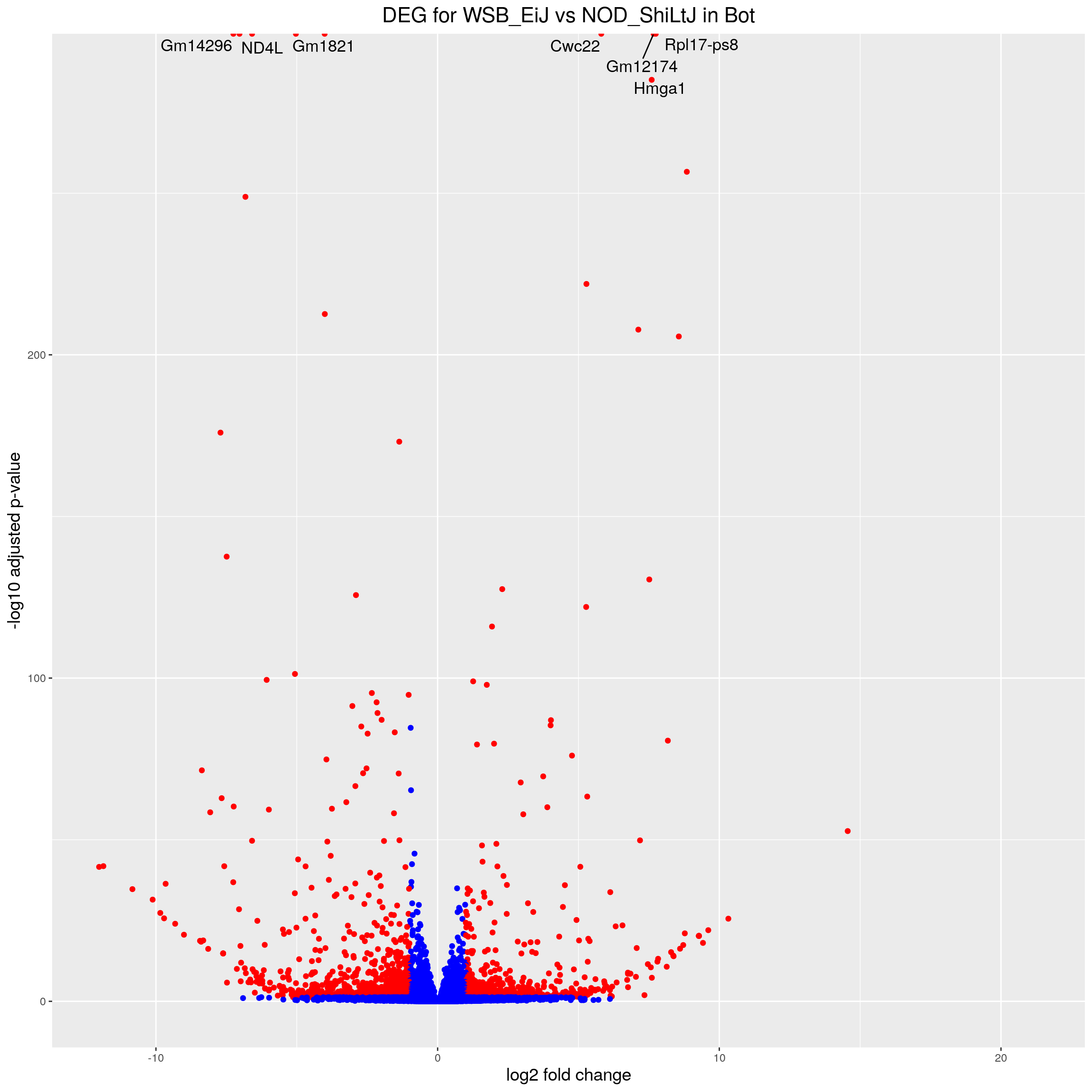
#heatmap
# Extract normalized expression for significant genes fdr < 0.05 & abs(log2FoldChange) >= 1)
normalized_counts_sig.strain.in.Bot <- normalized_counts %>%
filter(gene %in% rownames(subset(resSig.strain.in.Bot, padj < 0.05 & abs(log2FoldChange) >= 1))) %>%
dplyr::select(-1) %>%
dplyr::select(contains("Bot"))
### Set a color palette
heat_colors <- brewer.pal(6, "YlOrRd")
#annotation
df <- as.data.frame(colData(ddsMat)[,c("Strain","Tissue")]) %>%
filter(Tissue == "Bot")
### Run pheatmap using the metadata data frame for the annotation
sig.strain.in.Bot.plot <- pheatmap(as.matrix(normalized_counts_sig.strain.in.Bot),
color = heat_colors,
cluster_rows = T,
show_rownames = F,
annotation_col = df,
annotation_colors = list(Strain = c(NOD_ShiLtJ = "#0064C9",
WSB_EiJ ="#B10DC9"),
Tissue = c(Bot = "#96ca00",
NTS = "#ff9289")),
border_color = NA,
fontsize = 10,
scale = "row",
fontsize_row = 10,
height = 20, legend = FALSE, annotation_legend = FALSE, annotation_names_col = FALSE,
#main = "Heatmap of the top DEGs in WSB_EiJ vs NOD_ShiLtJ in Bot (fdr < 0.05 & abs(log2FoldChange) >= 1)"
)
sig.strain.in.Bot.plot
#enrichment analysis for res.tab.strain.in.Bot-------
dbs <- c("WikiPathways_2019_Mouse",
"GO_Biological_Process_2021",
"GO_Cellular_Component_2021",
"GO_Molecular_Function_2021",
"KEGG_2019_Mouse",
"Mouse_Gene_Atlas",
"MGI_Mammalian_Phenotype_Level_4_2019")
#results (fdr < 0.05)------
resSig.strain.in.Bot.tab <- resSig.strain.in.Bot %>%
data.frame() %>%
rownames_to_column(var="ENSEMBL") %>%
as_tibble() %>%
left_join(genes)Joining, by = "ENSEMBL"#up-regulated genes WSB_EiJ vs NOD_ShiLtJ in Bot ---------------------------
up.genes <- resSig.strain.in.Bot.tab %>%
filter(log2FoldChange > 0) %>%
pull(SYMBOL)
#up-regulated genes enrichment
up.genes.enriched <- enrichr(as.character(na.omit(up.genes)), dbs)Uploading data to Enrichr... Done.
Querying WikiPathways_2019_Mouse... Done.
Querying GO_Biological_Process_2021... Done.
Querying GO_Cellular_Component_2021... Done.
Querying GO_Molecular_Function_2021... Done.
Querying KEGG_2019_Mouse... Done.
Querying Mouse_Gene_Atlas... Done.
Querying MGI_Mammalian_Phenotype_Level_4_2019... Done.
Parsing results... Done.for (j in 1:length(up.genes.enriched)){
up.genes.enriched[[j]] <- cbind(data.frame(Library = names(up.genes.enriched)[j]),up.genes.enriched[[j]])
}
up.genes.enriched <- do.call(rbind.data.frame, up.genes.enriched) %>%
filter(Adjusted.P.value <= 0.05) %>%
mutate(logpvalue = -log10(P.value)) %>%
arrange(desc(logpvalue))
#display up.genes.enriched
DT::datatable(up.genes.enriched,filter = list(position = 'top', clear = FALSE),
options = list(pageLength = 40, scrollY = "300px", scrollX = "40px"))#barpot
up.genes.enriched.plot.in.Bot <- up.genes.enriched %>%
filter(Adjusted.P.value <= 0.01) %>%
mutate(Term = fct_reorder(Term, -logpvalue)) %>%
ggplot(data = ., aes(x = Term, y = logpvalue, fill = Library, label = Overlap)) +
geom_bar(stat = "identity") +
geom_text(position = position_dodge(width = 0.9),
hjust = 0) +
theme_bw() +
ylab("-log(p.value)") +
xlab("") +
ggtitle("Enrichment of up-regulated genes for WSB_EiJ vs NOD_ShiLtJ \nin Bot (Adjusted.P.value <= 0.01)") +
theme(plot.background = element_blank() ,
panel.border = element_blank(),
panel.background = element_blank(),
#legend.position = "none",
plot.title = element_text(hjust = 0),
panel.grid.major = element_blank(),
panel.grid.minor = element_blank()) +
theme(axis.line = element_line(color = 'black')) +
theme(axis.title.x = element_text(size = 12, vjust=-0.5)) +
theme(axis.title.y = element_text(size = 12, vjust= 1.0)) +
theme(axis.text = element_text(size = 12)) +
theme(plot.title = element_text(size = 12)) +
coord_flip()
up.genes.enriched.plot.in.Bot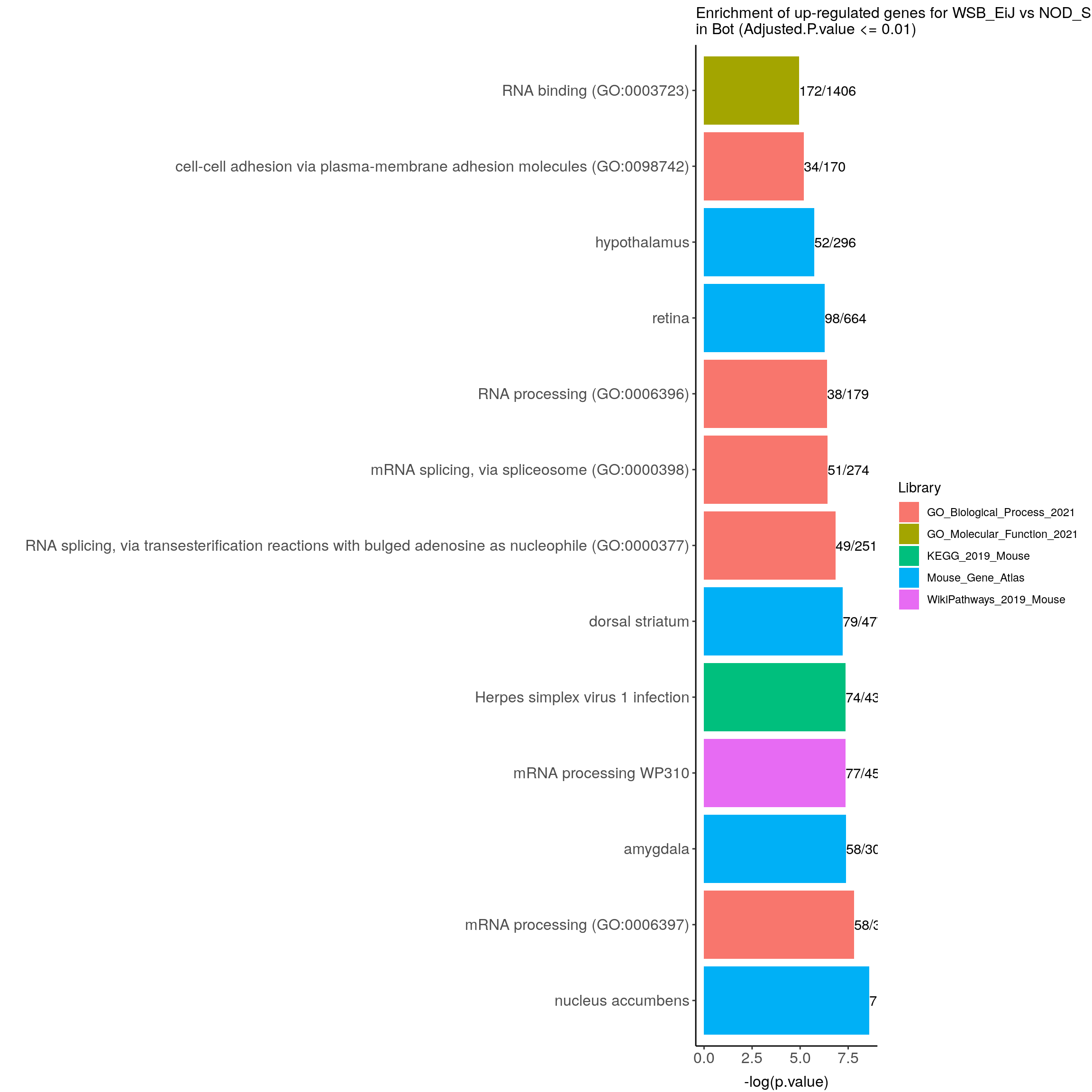
#down-regulated genes WSB_EiJ vs NOD_ShiLtJ in Bot---------------------------
down.genes <- resSig.strain.in.Bot.tab %>%
filter(log2FoldChange < 0) %>%
pull(SYMBOL)
#down-regulated genes enrichment
down.genes.enriched <- enrichr(as.character(na.omit(down.genes)), dbs)Uploading data to Enrichr... Done.
Querying WikiPathways_2019_Mouse... Done.
Querying GO_Biological_Process_2021... Done.
Querying GO_Cellular_Component_2021... Done.
Querying GO_Molecular_Function_2021... Done.
Querying KEGG_2019_Mouse... Done.
Querying Mouse_Gene_Atlas... Done.
Querying MGI_Mammalian_Phenotype_Level_4_2019... Done.
Parsing results... Done.for (j in 1:length(down.genes.enriched)){
down.genes.enriched[[j]] <- cbind(data.frame(Library = names(down.genes.enriched)[j]),down.genes.enriched[[j]])
}
down.genes.enriched <- do.call(rbind.data.frame, down.genes.enriched) %>%
filter(Adjusted.P.value <= 0.05) %>%
mutate(logpvalue = -log10(P.value)) %>%
arrange(desc(logpvalue))
#display down.genes.enriched
DT::datatable(down.genes.enriched,filter = list(position = 'top', clear = FALSE),
options = list(pageLength = 40, scrollY = "300px", scrollX = "40px"))#barpot
down.genes.enriched.plot.in.Bot <- down.genes.enriched %>%
filter(Adjusted.P.value <= 0.001) %>%
mutate(Term = fct_reorder(Term, -logpvalue)) %>%
ggplot(data = ., aes(x = Term, y = logpvalue, fill = Library, label = Overlap)) +
geom_bar(stat = "identity") +
geom_text(position = position_dodge(width = 0.9),
hjust = 0) +
theme_bw() +
ylab("-log(p.value)") +
xlab("") +
ggtitle("Enrichment of down-regulated genes for WSB_EiJ vs NOD_ShiLtJ \nin Bot (Adjusted.P.value <= 0.001)") +
theme(plot.background = element_blank() ,
panel.border = element_blank(),
panel.background = element_blank(),
#legend.position = "none",
plot.title = element_text(hjust = 0),
panel.grid.major = element_blank(),
panel.grid.minor = element_blank()) +
theme(axis.line = element_line(color = 'black')) +
theme(axis.title.x = element_text(size = 12, vjust=-0.5)) +
theme(axis.title.y = element_text(size = 12, vjust= 1.0)) +
theme(axis.text = element_text(size = 12)) +
theme(plot.title = element_text(size = 12)) +
coord_flip()
down.genes.enriched.plot.in.Bot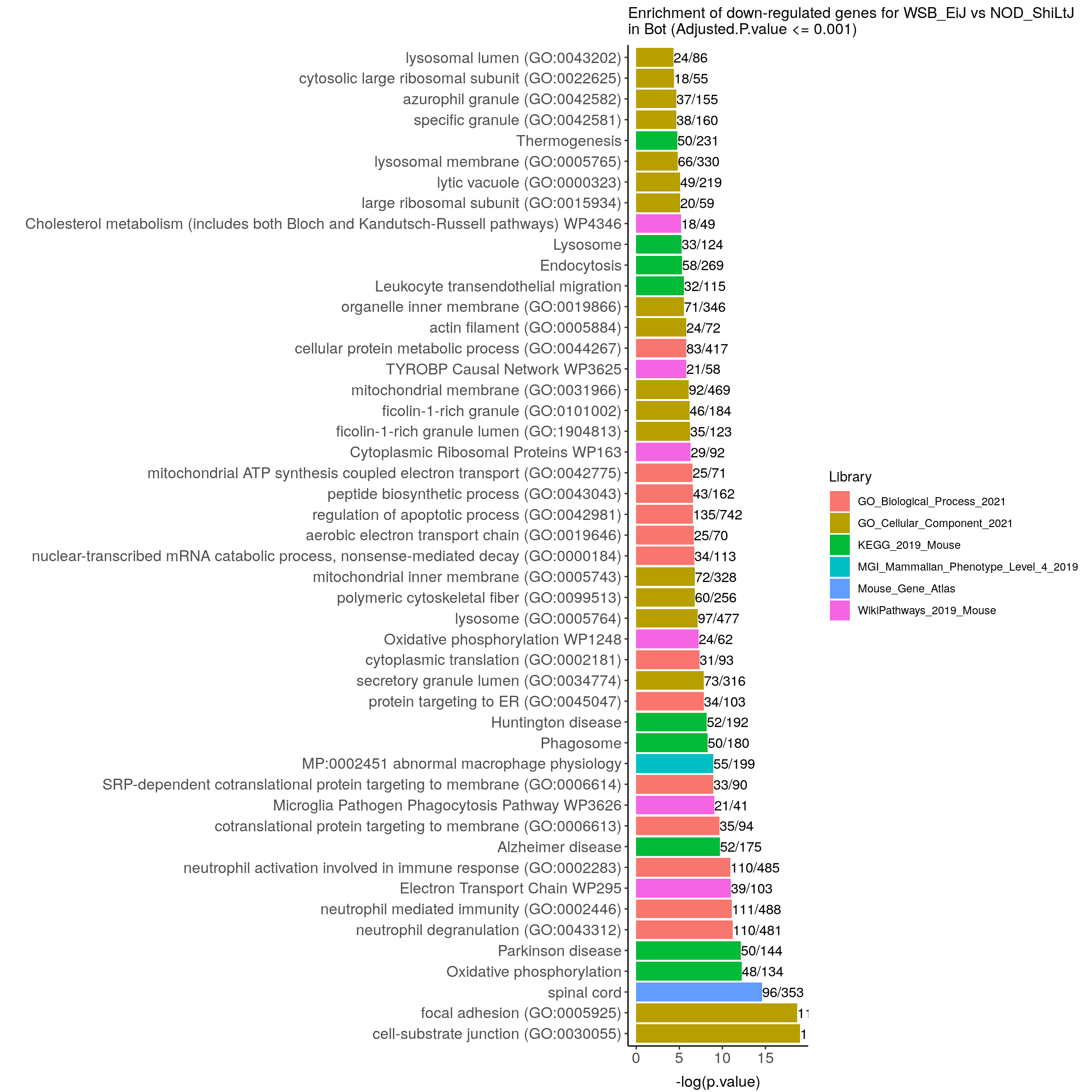
The effect of Strain in NTS
#This is, by definition, the main effect plus the interaction term
#Building the results table
res.tab.strain.in.NTS <- results(res, list(c("Strain_WSB_EiJ_vs_NOD_ShiLtJ",
"TissueNTS.StrainWSB_EiJ")), alpha = 0.05)
summary(res.tab.strain.in.NTS)
out of 27095 with nonzero total read count
adjusted p-value < 0.05
LFC > 0 (up) : 1845, 6.8%
LFC < 0 (down) : 2472, 9.1%
outliers [1] : 42, 0.16%
low counts [2] : 2618, 9.7%
(mean count < 1)
[1] see 'cooksCutoff' argument of ?results
[2] see 'independentFiltering' argument of ?resultstable(res.tab.strain.in.NTS$padj < 0.05)
FALSE TRUE
20118 4317 #We subset the results table to these genes and then sort it by the log2 fold change estimate to get the significant genes with the strongest down-regulation:
resSig.strain.in.NTS <- subset(res.tab.strain.in.NTS, padj < 0.05)
head(resSig.strain.in.NTS[order(resSig.strain.in.NTS$log2FoldChange), ])log2 fold change (MLE): Strain_WSB_EiJ_vs_NOD_ShiLtJ+TissueNTS.StrainWSB_EiJ effect
Wald test p-value: Strain_WSB_EiJ_vs_NOD_ShiLtJ+TissueNTS.StrainWSB_EiJ effect
DataFrame with 6 rows and 6 columns
baseMean log2FoldChange lfcSE stat pvalue
<numeric> <numeric> <numeric> <numeric> <numeric>
ENSMUSG00000092365 362.6730 -12.0816 0.841603 -14.35546 9.84684e-47
ENSMUSG00000053038 463.7134 -11.7139 0.853802 -13.71973 7.73574e-43
ENSMUSG00000066553 173.8310 -10.5182 0.842003 -12.49183 8.27281e-36
ENSMUSG00000079018 258.6623 -10.4881 0.849183 -12.35076 4.82547e-35
ENSMUSG00000020713 66.0074 -10.4068 2.991591 -3.47867 5.03908e-04
ENSMUSG00000101878 99.9184 -10.3282 0.857558 -12.04372 2.09311e-33
padj
<numeric>
ENSMUSG00000092365 2.93424e-44
ENSMUSG00000053038 2.05460e-40
ENSMUSG00000066553 1.78890e-33
ENSMUSG00000079018 9.82587e-33
ENSMUSG00000020713 4.99108e-03
ENSMUSG00000101878 3.93424e-31# with the strongest up-regulation:
head(resSig.strain.in.NTS[order(resSig.strain.in.NTS$log2FoldChange, decreasing = TRUE), ])log2 fold change (MLE): Strain_WSB_EiJ_vs_NOD_ShiLtJ+TissueNTS.StrainWSB_EiJ effect
Wald test p-value: Strain_WSB_EiJ_vs_NOD_ShiLtJ+TissueNTS.StrainWSB_EiJ effect
DataFrame with 6 rows and 6 columns
baseMean log2FoldChange lfcSE stat pvalue
<numeric> <numeric> <numeric> <numeric> <numeric>
ENSMUSG00000094306 2237.4111 13.11303 0.822463 15.9436 3.15564e-57
ENSMUSG00000094518 138.1547 10.58628 0.867647 12.2011 3.06495e-34
ENSMUSG00000103706 105.4107 10.10710 0.853250 11.8454 2.27291e-32
ENSMUSG00000096039 109.3540 10.07094 0.852302 11.8162 3.22050e-32
ENSMUSG00000021908 1579.3642 9.76553 0.323883 30.1514 1.02854e-199
ENSMUSG00000083773 42.0801 8.91116 0.868295 10.2628 1.03631e-24
padj
<numeric>
ENSMUSG00000094306 1.15087e-54
ENSMUSG00000094518 5.99136e-32
ENSMUSG00000103706 4.17584e-30
ENSMUSG00000096039 5.82911e-30
ENSMUSG00000021908 1.57077e-196
ENSMUSG00000083773 1.40680e-22#Visualization for res.tab.strain.in.NTS------
#Volcano plot
## Obtain logical vector regarding whether padj values are less than 0.05
threshold_OE <- (res.tab.strain.in.NTS$padj < 0.05 & !is.na(res.tab.strain.in.NTS$padj) & abs(res.tab.strain.in.NTS$log2FoldChange) >= 1)
## Determine the number of TRUE values
length(which(threshold_OE))[1] 1481## Add logical vector as a column (threshold) to the res.tab.strain.in.NTS
res.tab.strain.in.NTS$threshold <- threshold_OE
## Sort by ordered padj
res.tab.strain.in.NTS_ordered <- res.tab.strain.in.NTS %>%
data.frame() %>%
rownames_to_column(var="ENSEMBL") %>%
arrange(padj) %>%
mutate(genelabels = "") %>%
as_tibble() %>%
left_join(genes)Joining, by = "ENSEMBL"## Create a column to indicate which genes to label
res.tab.strain.in.NTS_ordered$genelabels[1:10] <- res.tab.strain.in.NTS_ordered$SYMBOL[1:10]
#display res.tab.strain.in.NTS_ordered
DT::datatable(res.tab.strain.in.NTS_ordered[res.tab.strain.in.NTS_ordered$threshold,],
filter = list(position = 'top', clear = FALSE),
options = list(pageLength = 40, scrollY = "300px", scrollX = "40px"),
caption = htmltools::tags$caption(style = 'caption-side: top; text-align: left; color:black; font-size:200% ;','DEG for WSB_EiJ vs NOD_ShiLtJ in NTS (fdr < 0.05)'))#Volcano plot
volcano.plot.strain.in.NTS <- ggplot(res.tab.strain.in.NTS_ordered) +
geom_point(aes(x = log2FoldChange, y = -log10(padj), colour = threshold)) +
scale_color_manual(values=c("blue", "red")) +
geom_text_repel(aes(x = log2FoldChange, y = -log10(padj),
label = genelabels,
size = 3.5)) +
ggtitle("DEG for WSB_EiJ vs NOD_ShiLtJ in NTS") +
xlab("log2 fold change") +
ylab("-log10 adjusted p-value") +
theme(legend.position = "none",
plot.title = element_text(size = rel(1.5), hjust = 0.5),
axis.title = element_text(size = rel(1.25)))
print(volcano.plot.strain.in.NTS)Warning: Removed 2660 rows containing missing values (geom_point).Warning: Removed 2663 rows containing missing values (geom_text_repel).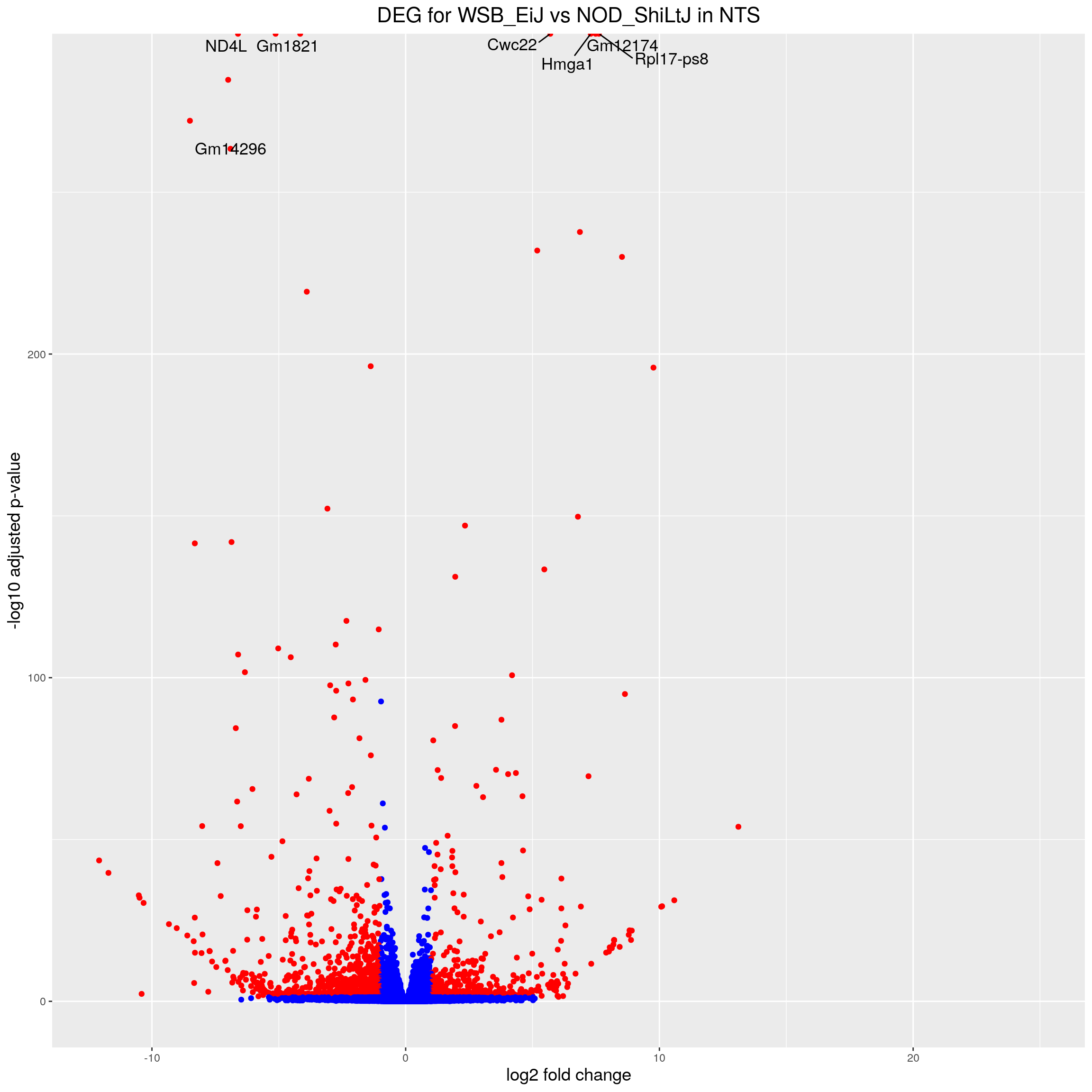
#heatmap
# Extract normalized expression for significant genes fdr < 0.05 & abs(log2FoldChange) >= 1)
normalized_counts_sig.strain.in.NTS <- normalized_counts %>%
filter(gene %in% rownames(subset(resSig.strain.in.NTS, padj < 0.05 & abs(log2FoldChange) >= 1))) %>%
dplyr::select(-1) %>%
dplyr::select(contains("NTS"))
### Set a color palette
heat_colors <- brewer.pal(6, "YlOrRd")
#annotation
df <- as.data.frame(colData(ddsMat)[,c("Strain","Tissue")]) %>%
filter(Tissue == "NTS")
### Run pheatmap using the metadata data frame for the annotation
sig.strain.in.NTS.plot <- pheatmap(as.matrix(normalized_counts_sig.strain.in.NTS),
color = heat_colors,
cluster_rows = T,
show_rownames = F,
annotation_col = df,
annotation_colors = list(Strain = c(NOD_ShiLtJ = "#0064C9",
WSB_EiJ ="#B10DC9"),
Tissue = c(Bot = "#96ca00",
NTS = "#ff9289")),
border_color = NA,
fontsize = 10,
scale = "row",
fontsize_row = 10,
height = 20, #legend = FALSE, annotation_legend = FALSE, annotation_names_col = FALSE,
#main = "Heatmap of the top DEGs in WSB_EiJ vs NOD_ShiLtJ in NTS (fdr < 0.05 & abs(log2FoldChange) >= 1)"
)
sig.strain.in.NTS.plot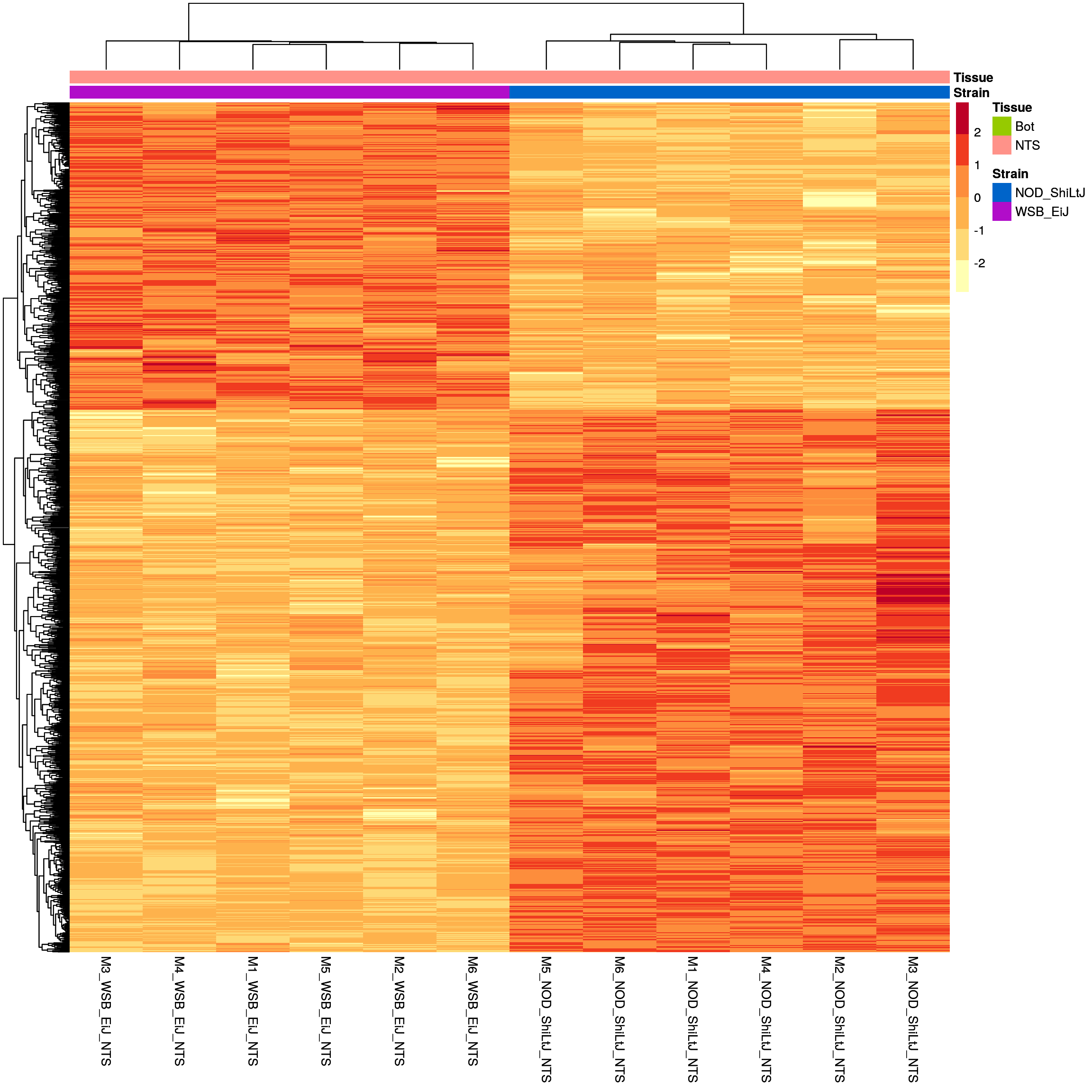
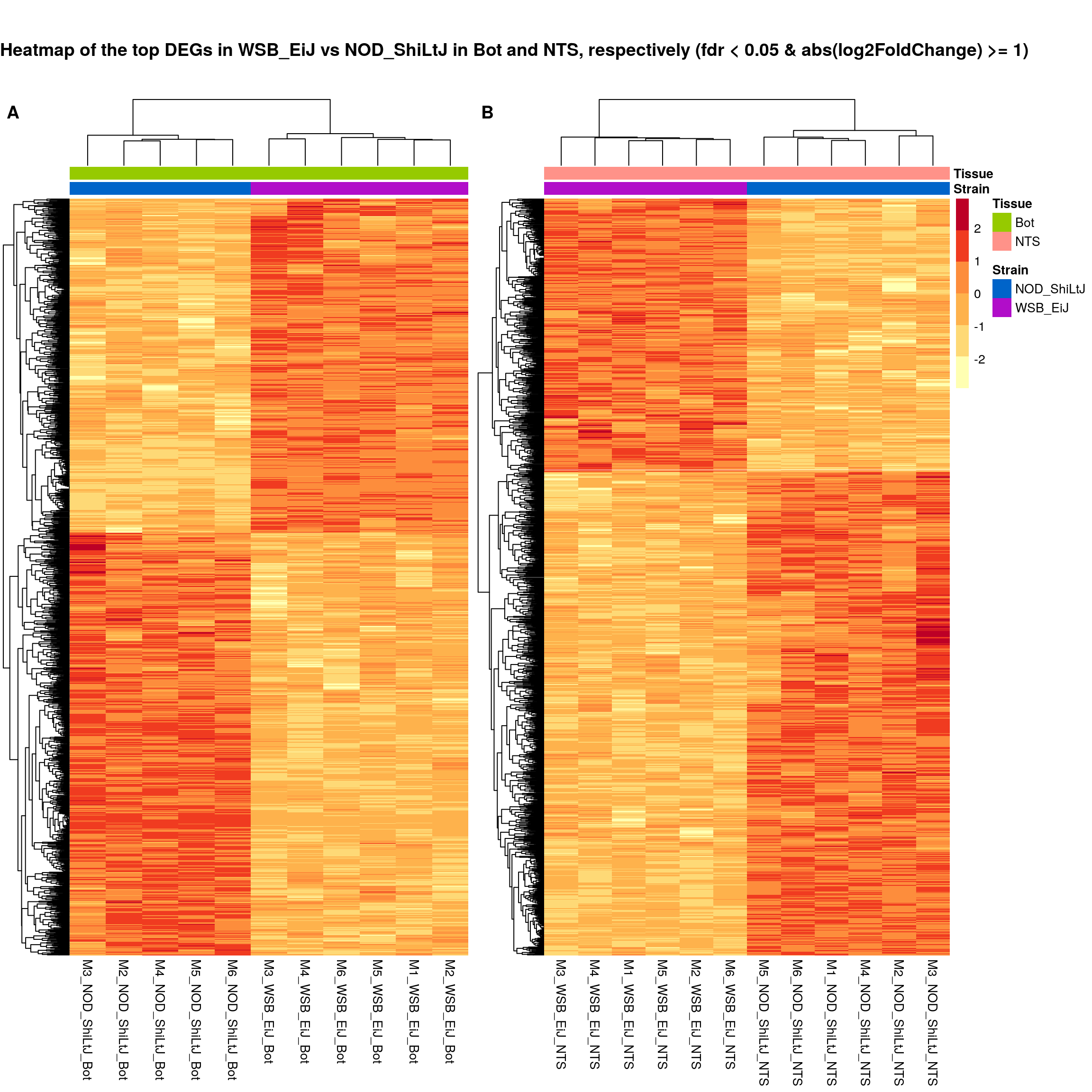
#plot sig.strain.in.Bot.plot and sig.strain.in.NTS.plot together-------
ht.map2.plot = plot_grid(as.grob(sig.strain.in.Bot.plot),
as.grob(sig.strain.in.NTS.plot),
align = "h", rel_widths = c(1, 1.3),
labels = c('A', 'B'))
#add title
# now add the title
title <- ggdraw() +
draw_label(
"Heatmap of the top DEGs in WSB_EiJ vs NOD_ShiLtJ in Bot and NTS, respectively (fdr < 0.05 & abs(log2FoldChange) >= 1)",
fontface = 'bold',
x = 0,
hjust = 0
)
plot_grid(
title,
ht.map2.plot,
ncol = 1,
# rel_heights values control vertical title margins
rel_heights = c(0.1, 1)
)
| Version | Author | Date |
|---|---|---|
| f6ccb3e | xhyuo | 2021-07-01 |
#logFC heatmap on both Bot and NTS top DEGs-----
restop.tab.in.Bot.NTS <- full_join(res.tab.strain.in.Bot_ordered,
res.tab.strain.in.NTS_ordered,
by = c("ENSEMBL", "SYMBOL")) %>%
filter((ENSEMBL %in% res.tab.strain.in.Bot_ordered$ENSEMBL[1:30]) | (ENSEMBL %in% res.tab.strain.in.NTS_ordered$ENSEMBL[1:30]))
restop.tab.in.Bot.NTS.mat <- as.matrix(restop.tab.in.Bot.NTS[, c("log2FoldChange.x", "log2FoldChange.y")])
rownames(restop.tab.in.Bot.NTS.mat) <-
ifelse(is.na(restop.tab.in.Bot.NTS$SYMBOL),
restop.tab.in.Bot.NTS$ENSEMBL,
paste0(restop.tab.in.Bot.NTS$SYMBOL,":", restop.tab.in.Bot.NTS$ENSEMBL))
colnames(restop.tab.in.Bot.NTS.mat) <- c("Bot", "NTS")
#heatmap
### Run pheatmap using the metadata data frame for the annotation
pheatmap(restop.tab.in.Bot.NTS.mat,
color = colorpanel(1000, "blue", "white", "red"),
cluster_rows = T,
show_rownames = T,
border_color = NA,
fontsize = 10,
fontsize_row = 8,
height = 25,
main = "Heatmap of log2FoldChange for the top 30 DEGs in Bot and NTS")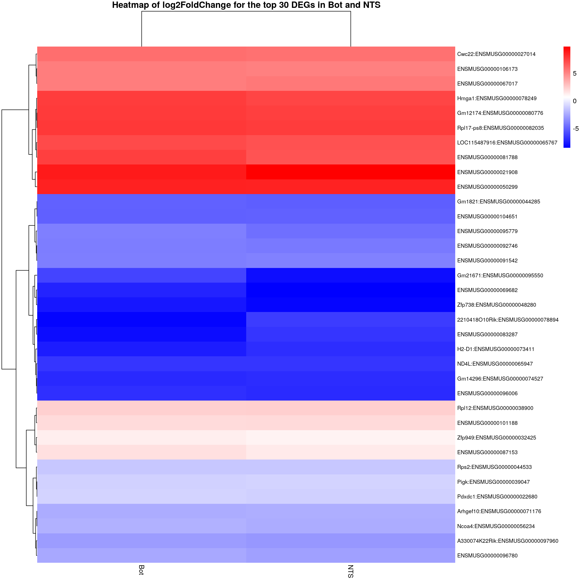
#enrichment analysis for res.tab.strain.in.NTS-------
dbs <- c("WikiPathways_2019_Mouse",
"GO_Biological_Process_2021",
"GO_Cellular_Component_2021",
"GO_Molecular_Function_2021",
"KEGG_2019_Mouse",
"Mouse_Gene_Atlas",
"MGI_Mammalian_Phenotype_Level_4_2019")
#results (fdr < 0.05)------
resSig.strain.in.NTS.tab <- resSig.strain.in.NTS %>%
data.frame() %>%
rownames_to_column(var="ENSEMBL") %>%
as_tibble() %>%
left_join(genes)Joining, by = "ENSEMBL"#up-regulated genes WSB_EiJ vs NOD_ShiLtJ in NTS ---------------------------
up.genes <- resSig.strain.in.NTS.tab %>%
filter(log2FoldChange > 0) %>%
pull(SYMBOL)
#up-regulated genes enrichment
up.genes.enriched <- enrichr(as.character(na.omit(up.genes)), dbs)Uploading data to Enrichr... Done.
Querying WikiPathways_2019_Mouse... Done.
Querying GO_Biological_Process_2021... Done.
Querying GO_Cellular_Component_2021... Done.
Querying GO_Molecular_Function_2021... Done.
Querying KEGG_2019_Mouse... Done.
Querying Mouse_Gene_Atlas... Done.
Querying MGI_Mammalian_Phenotype_Level_4_2019... Done.
Parsing results... Done.for (j in 1:length(up.genes.enriched)){
up.genes.enriched[[j]] <- cbind(data.frame(Library = names(up.genes.enriched)[j]),up.genes.enriched[[j]])
}
up.genes.enriched <- do.call(rbind.data.frame, up.genes.enriched) %>%
filter(Adjusted.P.value <= 0.2) %>%
mutate(logpvalue = -log10(P.value)) %>%
arrange(desc(logpvalue))
#display up.genes.enriched
DT::datatable(up.genes.enriched,filter = list(position = 'top', clear = FALSE),
options = list(pageLength = 40, scrollY = "300px", scrollX = "40px"))#barpot
up.genes.enriched.plot.in.NTS <- up.genes.enriched %>%
filter(Adjusted.P.value <= 0.2) %>%
mutate(Term = fct_reorder(Term, -logpvalue)) %>%
ggplot(data = ., aes(x = Term, y = logpvalue, fill = Library, label = Overlap)) +
geom_bar(stat = "identity") +
geom_text(position = position_dodge(width = 0.9),
hjust = 0) +
theme_bw() +
ylab("-log(p.value)") +
xlab("") +
ggtitle("Enrichment of up-regulated genes for WSB_EiJ vs NOD_ShiLtJ \nin NTS (Adjusted.P.value <= 0.2)") +
theme(plot.background = element_blank() ,
panel.border = element_blank(),
panel.background = element_blank(),
#legend.position = "none",
plot.title = element_text(hjust = 0),
panel.grid.major = element_blank(),
panel.grid.minor = element_blank()) +
theme(axis.line = element_line(color = 'black')) +
theme(axis.title.x = element_text(size = 12, vjust=-0.5)) +
theme(axis.title.y = element_text(size = 12, vjust= 1.0)) +
theme(axis.text = element_text(size = 12)) +
theme(plot.title = element_text(size = 12)) +
coord_flip()
up.genes.enriched.plot.in.NTS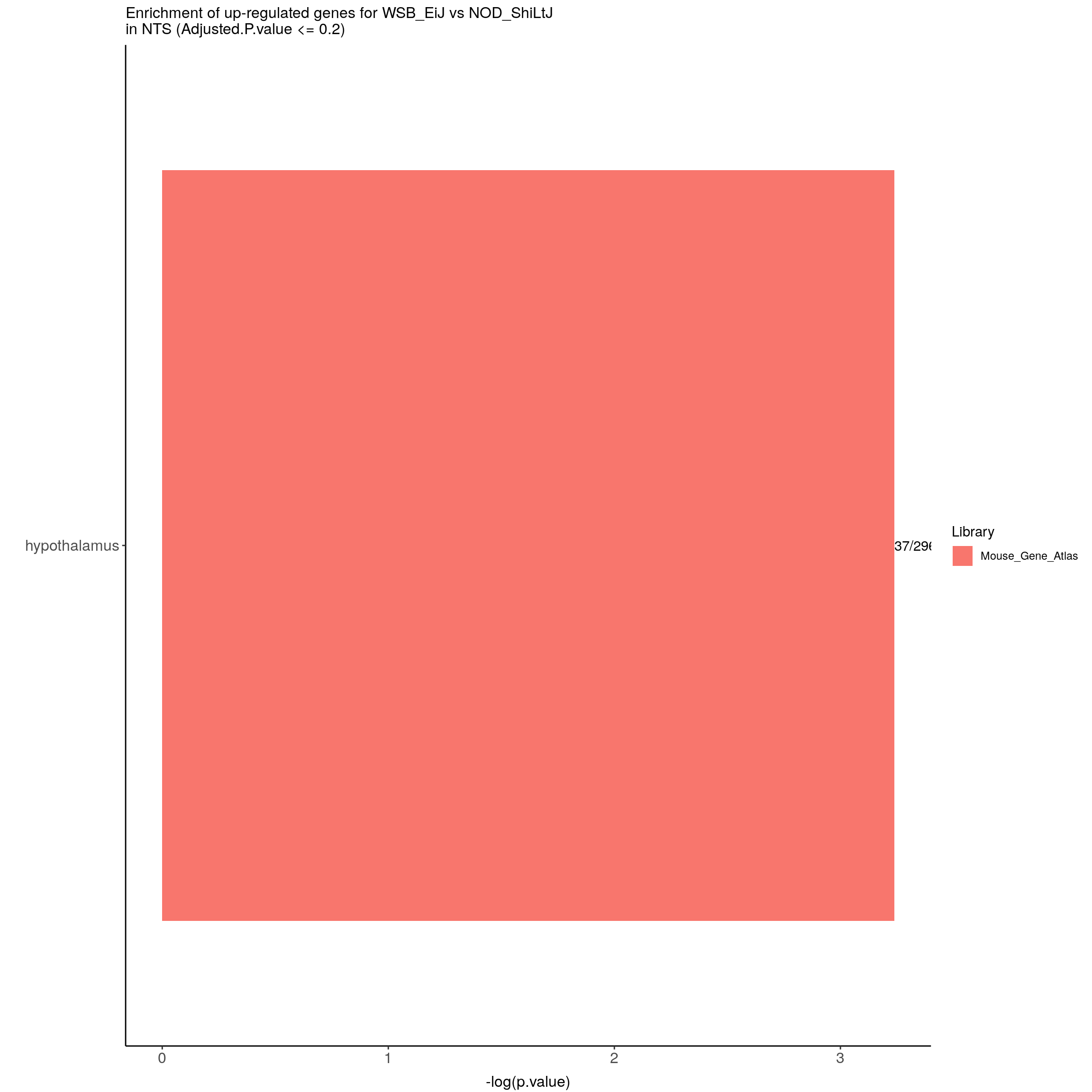
#down-regulated genes WSB_EiJ vs NOD_ShiLtJ in NTS---------------------------
down.genes <- resSig.strain.in.NTS.tab %>%
filter(log2FoldChange < 0) %>%
pull(SYMBOL)
#down-regulated genes enrichment
down.genes.enriched <- enrichr(as.character(na.omit(down.genes)), dbs)Uploading data to Enrichr... Done.
Querying WikiPathways_2019_Mouse... Done.
Querying GO_Biological_Process_2021... Done.
Querying GO_Cellular_Component_2021... Done.
Querying GO_Molecular_Function_2021... Done.
Querying KEGG_2019_Mouse... Done.
Querying Mouse_Gene_Atlas... Done.
Querying MGI_Mammalian_Phenotype_Level_4_2019... Done.
Parsing results... Done.for (j in 1:length(down.genes.enriched)){
down.genes.enriched[[j]] <- cbind(data.frame(Library = names(down.genes.enriched)[j]),down.genes.enriched[[j]])
}
down.genes.enriched <- do.call(rbind.data.frame, down.genes.enriched) %>%
filter(Adjusted.P.value <= 0.05) %>%
mutate(logpvalue = -log10(P.value)) %>%
arrange(desc(logpvalue))
#display down.genes.enriched
DT::datatable(down.genes.enriched,filter = list(position = 'top', clear = FALSE),
options = list(pageLength = 40, scrollY = "300px", scrollX = "40px"))#barpot
down.genes.enriched.plot.in.NTS <- down.genes.enriched %>%
filter(Adjusted.P.value <= 0.001) %>%
mutate(Term = fct_reorder(Term, -logpvalue)) %>%
ggplot(data = ., aes(x = Term, y = logpvalue, fill = Library, label = Overlap)) +
geom_bar(stat = "identity") +
geom_text(position = position_dodge(width = 0.9),
hjust = 0) +
theme_bw() +
ylab("-log(p.value)") +
xlab("") +
ggtitle("Enrichment of down-regulated genes for WSB_EiJ vs NOD_ShiLtJ \nin NTS (Adjusted.P.value <= 0.001)") +
theme(plot.background = element_blank() ,
panel.border = element_blank(),
panel.background = element_blank(),
#legend.position = "none",
plot.title = element_text(hjust = 0),
panel.grid.major = element_blank(),
panel.grid.minor = element_blank()) +
theme(axis.line = element_line(color = 'black')) +
theme(axis.title.x = element_text(size = 12, vjust=-0.5)) +
theme(axis.title.y = element_text(size = 12, vjust= 1.0)) +
theme(axis.text = element_text(size = 12)) +
theme(plot.title = element_text(size = 12)) +
coord_flip()
down.genes.enriched.plot.in.NTS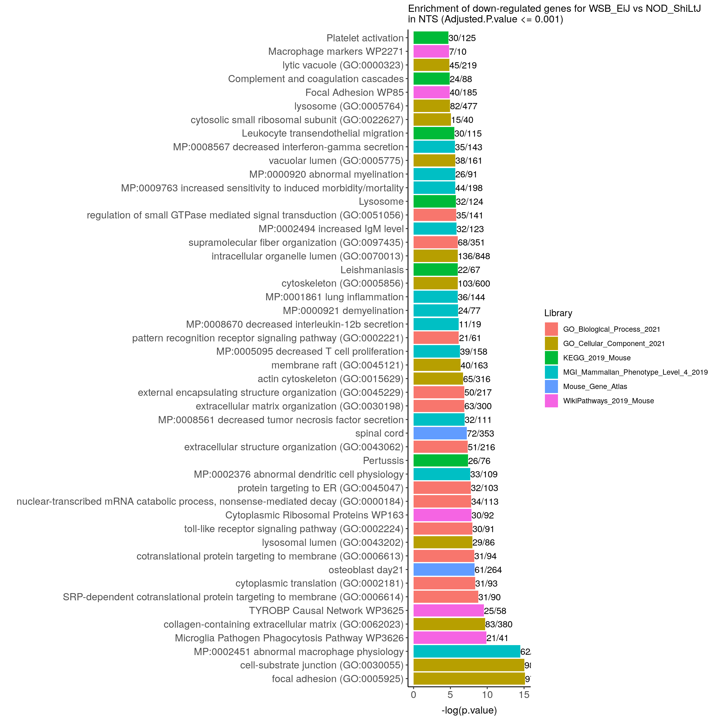
| Version | Author | Date |
|---|---|---|
| f6ccb3e | xhyuo | 2021-07-01 |
Differential expression analysis with interaction term and one outlier removed
design(ddsMat) <- ~Tissue + Strain + Tissue:Strain
ddsMat <- ddsMat[,-which(colnames(ddsMat) == "M6_WSB_EiJ_NTS")] # remove outlier
#Running the differential expression pipeline
res <- DESeq(ddsMat)estimating size factorsestimating dispersionsgene-wise dispersion estimatesmean-dispersion relationshipfinal dispersion estimatesfitting model and testingresultsNames(res)[1] "Intercept" "Tissue_NTS_vs_Bot"
[3] "Strain_WSB_EiJ_vs_NOD_ShiLtJ" "TissueNTS.StrainWSB_EiJ" The effect of Strain in Bot with one outlier removed
#in Bot, WSB_EiJ compared with NOD_ShiLtJ
#Building the results table
res.tab.strain.in.Bot <- results(res, contrast=c("Strain","WSB_EiJ","NOD_ShiLtJ"), alpha = 0.05)
res.tab.strain.in.Botlog2 fold change (MLE): Strain WSB_EiJ vs NOD_ShiLtJ
Wald test p-value: Strain WSB EiJ vs NOD ShiLtJ
DataFrame with 27095 rows and 6 columns
baseMean log2FoldChange lfcSE stat pvalue
<numeric> <numeric> <numeric> <numeric> <numeric>
ENSMUSG00000000001 1122.2041 -0.1550374 0.0943166 -1.643797 0.100218
ENSMUSG00000000028 55.8600 -0.0403637 0.2944303 -0.137091 0.890959
ENSMUSG00000000031 20.3388 -0.0998453 0.6212381 -0.160720 0.872314
ENSMUSG00000000037 35.4552 0.4165333 0.3377470 1.233270 0.217475
ENSMUSG00000000049 7.5440 -0.1940756 0.8098794 -0.239635 0.810613
... ... ... ... ... ...
ENSMUSG00000108290 0.395370 0.590982 4.076612 0.144969 0.88473533
ENSMUSG00000108291 61.811893 0.310761 0.278456 1.116018 0.26441429
ENSMUSG00000108292 0.935794 2.234104 2.910916 0.767492 0.44278926
ENSMUSG00000108297 319.429146 0.390537 0.141350 2.762908 0.00572889
ENSMUSG00000108298 5.465225 1.401838 1.021689 1.372079 0.17003876
padj
<numeric>
ENSMUSG00000000001 0.258658
ENSMUSG00000000028 0.951465
ENSMUSG00000000031 0.942124
ENSMUSG00000000037 0.430213
ENSMUSG00000000049 0.911194
... ...
ENSMUSG00000108290 NA
ENSMUSG00000108291 0.4847265
ENSMUSG00000108292 NA
ENSMUSG00000108297 0.0321041
ENSMUSG00000108298 0.3665570summary(res.tab.strain.in.Bot)
out of 27093 with nonzero total read count
adjusted p-value < 0.05
LFC > 0 (up) : 2373, 8.8%
LFC < 0 (down) : 2637, 9.7%
outliers [1] : 40, 0.15%
low counts [2] : 2620, 9.7%
(mean count < 1)
[1] see 'cooksCutoff' argument of ?results
[2] see 'independentFiltering' argument of ?resultstable(res.tab.strain.in.Bot$padj < 0.05)
FALSE TRUE
19423 5010 #We subset the results table to these genes and then sort it by the log2 fold change estimate to get the significant genes with the strongest down-regulation:
resSig.strain.in.Bot <- subset(res.tab.strain.in.Bot, padj < 0.05)
head(resSig.strain.in.Bot[order(resSig.strain.in.Bot$log2FoldChange), ])log2 fold change (MLE): Strain WSB_EiJ vs NOD_ShiLtJ
Wald test p-value: Strain WSB EiJ vs NOD ShiLtJ
DataFrame with 6 rows and 6 columns
baseMean log2FoldChange lfcSE stat pvalue
<numeric> <numeric> <numeric> <numeric> <numeric>
ENSMUSG00000053038 482.1118 -12.01635 0.855678 -14.0431 8.49464e-45
ENSMUSG00000092365 377.0809 -11.86491 0.842412 -14.0844 4.73384e-45
ENSMUSG00000066553 180.7374 -10.83409 0.842800 -12.8549 8.07442e-38
ENSMUSG00000079018 268.8942 -10.11594 0.825467 -12.2548 1.58336e-34
ENSMUSG00000101878 103.8932 -9.84484 0.859982 -11.4477 2.41386e-30
ENSMUSG00000094891 68.0095 -9.70954 0.873970 -11.1097 1.12547e-28
padj
<numeric>
ENSMUSG00000053038 2.62721e-42
ENSMUSG00000092365 1.48285e-42
ENSMUSG00000066553 2.05502e-35
ENSMUSG00000079018 3.39354e-32
ENSMUSG00000101878 4.43443e-28
ENSMUSG00000094891 1.88346e-26# with the strongest up-regulation:
head(resSig.strain.in.Bot[order(resSig.strain.in.Bot$log2FoldChange, decreasing = TRUE), ])log2 fold change (MLE): Strain WSB_EiJ vs NOD_ShiLtJ
Wald test p-value: Strain WSB EiJ vs NOD ShiLtJ
DataFrame with 6 rows and 6 columns
baseMean log2FoldChange lfcSE stat pvalue
<numeric> <numeric> <numeric> <numeric> <numeric>
ENSMUSG00000094306 2169.6074 14.55941 0.922968 15.77455 4.65720e-56
ENSMUSG00000096039 105.1752 10.32233 0.933642 11.05599 2.05060e-28
ENSMUSG00000103706 101.2714 9.60973 0.934563 10.28259 8.44264e-25
ENSMUSG00000069083 63.3371 9.42139 1.014636 9.28549 1.60971e-20
ENSMUSG00000079247 53.7965 9.27700 0.940374 9.86523 5.88995e-23
ENSMUSG00000094125 53.7965 9.27700 0.940374 9.86523 5.88995e-23
padj
<numeric>
ENSMUSG00000094306 1.77796e-53
ENSMUSG00000096039 3.36257e-26
ENSMUSG00000103706 1.17874e-22
ENSMUSG00000069083 1.71747e-18
ENSMUSG00000079247 7.41800e-21
ENSMUSG00000094125 7.41800e-21#Visualization for res.tab.strain.in.Bot------
#Volcano plot
## Obtain logical vector regarding whether padj values are less than 0.05
threshold_OE <- (res.tab.strain.in.Bot$padj < 0.05 & !is.na(res.tab.strain.in.Bot$padj) & abs(res.tab.strain.in.Bot$log2FoldChange) >= 1)
## Determine the number of TRUE values
length(which(threshold_OE))[1] 1445## Add logical vector as a column (threshold) to the res.tab.strain.in.Bot
res.tab.strain.in.Bot$threshold <- threshold_OE
## Sort by ordered padj
res.tab.strain.in.Bot_ordered <- res.tab.strain.in.Bot %>%
data.frame() %>%
rownames_to_column(var="ENSEMBL") %>%
arrange(padj) %>%
mutate(genelabels = "") %>%
as_tibble() %>%
left_join(genes)Joining, by = "ENSEMBL"## Create a column to indicate which genes to label
res.tab.strain.in.Bot_ordered$genelabels[1:10] <- res.tab.strain.in.Bot_ordered$SYMBOL[1:10]
#display res.tab.strain.in.Bot_ordered
DT::datatable(res.tab.strain.in.Bot_ordered[(res.tab.strain.in.Bot_ordered$padj < 0.05 & !is.na(res.tab.strain.in.Bot_ordered$padj)), ],
filter = list(position = 'top', clear = FALSE),
extensions = 'Buttons',
options = list(dom = 'Blfrtip',
buttons = c('csv', 'excel'),
lengthMenu = list(c(10,25,50,-1),
c(10,25,50,"All")),
pageLength = 40,
scrollY = "300px",
scrollX = "40px"),
caption = htmltools::tags$caption(style = 'caption-side: top; text-align: left; color:black; font-size:200% ;','DEG for WSB_EiJ vs NOD_ShiLtJ in Bot (fdr < 0.05)'))write.csv(res.tab.strain.in.Bot_ordered[(res.tab.strain.in.Bot_ordered$padj < 0.05 & !is.na(res.tab.strain.in.Bot_ordered$padj)), ],
file = "data/rnaseq/DEG_WSB_vs_NOD_in_Bot_fdr_0.05_with_one_outlier_removed.csv",
row.names = F, quote = F)
#Volcano plot
volcano.plot.strain.in.Bot <- ggplot(res.tab.strain.in.Bot_ordered) +
  geom_point(aes(x = log2FoldChange, y = -log10(padj), colour = threshold)) +
  scale_color_manual(values=c("blue", "red")) +
  geom_text_repel(aes(x = log2FoldChange, y = -log10(padj),
                      label = genelabels,
                      size = 3.5)) +
  ggtitle("DEG for WSB_EiJ vs NOD_ShiLtJ in Bot") +
  xlab("log2 fold change") +
  ylab("-log10 adjusted p-value") +
  theme(legend.position = "none",
        plot.title = element_text(size = rel(1.5), hjust = 0.5),
        axis.title = element_text(size = rel(1.25)))
print(volcano.plot.strain.in.Bot)
Warning: Removed 2662 rows containing missing values (geom_point).Warning: Removed 2666 rows containing missing values (geom_text_repel).
| Version | Author | Date |
|---|---|---|
| f6ccb3e | xhyuo | 2021-07-01 |
#heatmap
# Extract normalized expression for significant genes fdr < 0.05 & abs(log2FoldChange) >= 1)
normalized_counts_sig.strain.in.Bot <- normalized_counts %>%
  filter(gene %in% rownames(subset(resSig.strain.in.Bot, padj < 0.05 & abs(log2FoldChange) >= 1))) %>%
  dplyr::select(-1) %>%
  dplyr::select(contains("Bot"))

### Set a color palette
heat_colors <- brewer.pal(6, "YlOrRd")
#annotation
df <- as.data.frame(colData(ddsMat)[,c("Strain","Tissue")]) %>%
  filter(Tissue == "Bot")
### Run pheatmap using the metadata data frame for the annotation
sig.strain.in.Bot.plot <- pheatmap(as.matrix(normalized_counts_sig.strain.in.Bot),
                                   color = heat_colors,
                                   cluster_rows = T,
                                   show_rownames = F,
                                   annotation_col  = df,
                                   annotation_colors = list(Strain = c(NOD_ShiLtJ = "#0064C9",
                                                                       WSB_EiJ    ="#B10DC9"),
                                                            Tissue = c(Bot = "#96ca00",
                                                                       NTS = "#ff9289")),
                                   border_color = NA,
                                   fontsize = 10,
                                   scale = "row",
                                   fontsize_row = 10,
                                   height = 20, legend = FALSE, annotation_legend = FALSE, annotation_names_col = FALSE,
                                   #main = "Heatmap of the top DEGs in WSB_EiJ vs NOD_ShiLtJ in Bot (fdr < 0.05 & abs(log2FoldChange) >= 1)"
                                   )
sig.strain.in.Bot.plot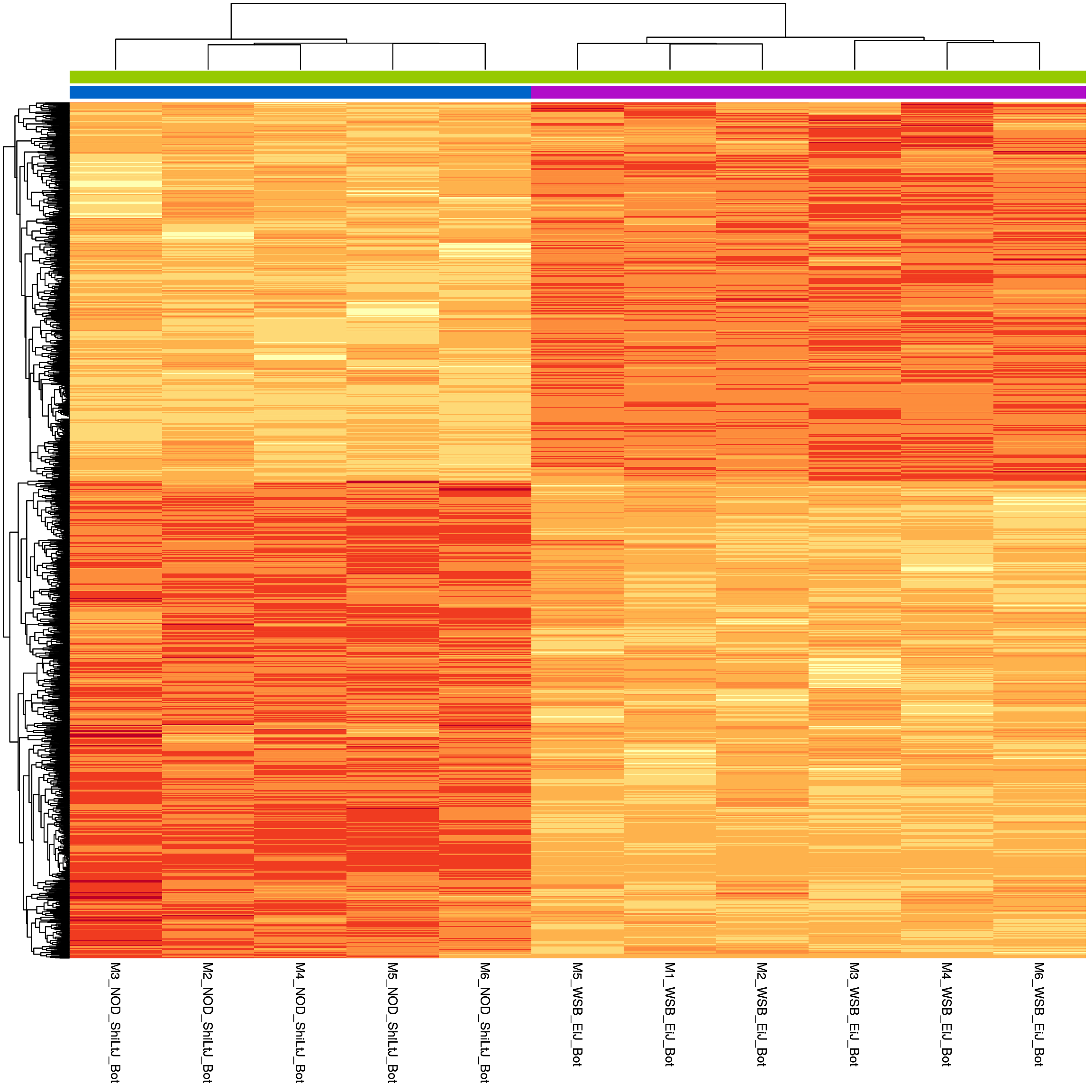
| Version | Author | Date |
|---|---|---|
| f6ccb3e | xhyuo | 2021-07-01 |
#enrichment analysis for res.tab.strain.in.Bot-------
dbs <- c("WikiPathways_2019_Mouse",
         "GO_Biological_Process_2021",
         "GO_Cellular_Component_2021",
         "GO_Molecular_Function_2021",
         "KEGG_2019_Mouse",
         "Mouse_Gene_Atlas",
         "MGI_Mammalian_Phenotype_Level_4_2019")

#results (fdr < 0.05)------
resSig.strain.in.Bot.tab <- resSig.strain.in.Bot %>%
  data.frame() %>%
  rownames_to_column(var="ENSEMBL") %>%
  as_tibble() %>%
  left_join(genes)
Joining, by = "ENSEMBL"#up-regulated genes WSB_EiJ vs NOD_ShiLtJ in Bot ---------------------------
up.genes <- resSig.strain.in.Bot.tab %>%
filter(log2FoldChange > 0) %>%
pull(SYMBOL)
#up-regulated genes enrichment
up.genes.enriched <- enrichr(as.character(na.omit(up.genes)), dbs)Uploading data to Enrichr... Done.
Querying WikiPathways_2019_Mouse... Done.
Querying GO_Biological_Process_2021... Done.
Querying GO_Cellular_Component_2021... Done.
Querying GO_Molecular_Function_2021... Done.
Querying KEGG_2019_Mouse... Done.
Querying Mouse_Gene_Atlas... Done.
Querying MGI_Mammalian_Phenotype_Level_4_2019... Done.
Parsing results... Done.for (j in 1:length(up.genes.enriched)){
up.genes.enriched[[j]] <- cbind(data.frame(Library = names(up.genes.enriched)[j]),up.genes.enriched[[j]])
}
up.genes.enriched <- do.call(rbind.data.frame, up.genes.enriched) %>%
filter(Adjusted.P.value <= 0.05) %>%
mutate(logpvalue = -log10(P.value)) %>%
arrange(desc(logpvalue))
#display up.genes.enriched
DT::datatable(up.genes.enriched,
filter = list(position = 'top', clear = FALSE),
extensions = 'Buttons',
options = list(dom = 'Blfrtip',
buttons = c('csv', 'excel'),
lengthMenu = list(c(10,25,50,-1),c(10,25,50,"All")),
pageLength = 40,
scrollY = "300px",
scrollX = "40px")
)#barpot
up.genes.enriched.plot.in.Bot <- up.genes.enriched %>%
filter(Adjusted.P.value <= 0.01) %>%
mutate(Term = fct_reorder(Term, -logpvalue)) %>%
ggplot(data = ., aes(x = Term, y = logpvalue, fill = Library, label = Overlap)) +
geom_bar(stat = "identity") +
geom_text(position = position_dodge(width = 0.9),
hjust = 0) +
theme_bw() +
ylab("-log(p.value)") +
xlab("") +
ggtitle("Enrichment of up-regulated genes for WSB_EiJ vs NOD_ShiLtJ \nin Bot (Adjusted.P.value <= 0.01)") +
theme(plot.background = element_blank() ,
panel.border = element_blank(),
panel.background = element_blank(),
#legend.position = "none",
plot.title = element_text(hjust = 0),
panel.grid.major = element_blank(),
panel.grid.minor = element_blank()) +
theme(axis.line = element_line(color = 'black')) +
theme(axis.title.x = element_text(size = 12, vjust=-0.5)) +
theme(axis.title.y = element_text(size = 12, vjust= 1.0)) +
theme(axis.text = element_text(size = 12)) +
theme(plot.title = element_text(size = 12)) +
coord_flip()
up.genes.enriched.plot.in.Bot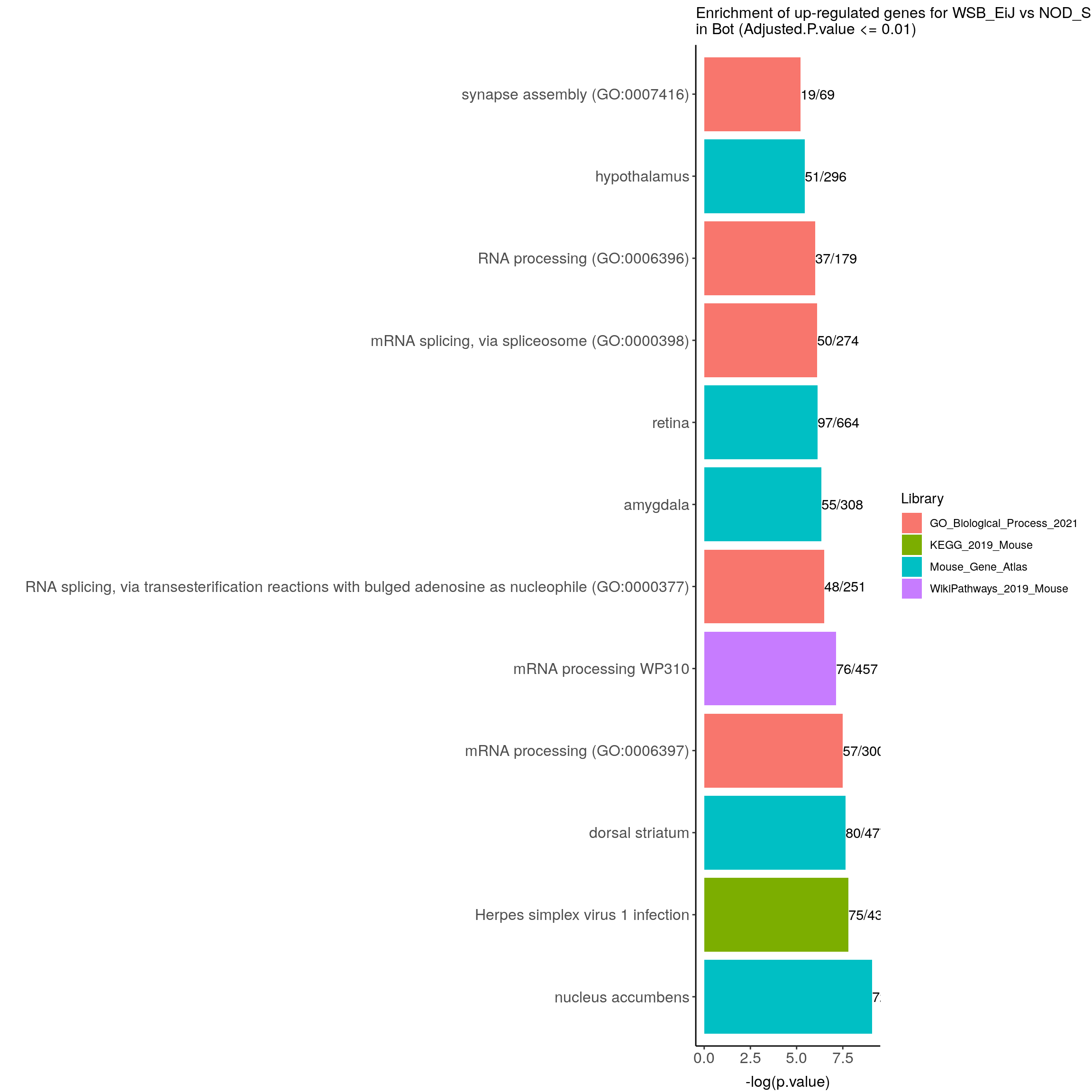
| Version | Author | Date |
|---|---|---|
| f6ccb3e | xhyuo | 2021-07-01 |
#down-regulated genes WSB_EiJ vs NOD_ShiLtJ in Bot---------------------------
down.genes <- resSig.strain.in.Bot.tab %>%
  filter(log2FoldChange < 0) %>%
  pull(SYMBOL)
#down-regulated genes enrichment
down.genes.enriched <- enrichr(as.character(na.omit(down.genes)), dbs)
Uploading data to Enrichr... Done.
Querying WikiPathways_2019_Mouse... Done.
Querying GO_Biological_Process_2021... Done.
Querying GO_Cellular_Component_2021... Done.
Querying GO_Molecular_Function_2021... Done.
Querying KEGG_2019_Mouse... Done.
Querying Mouse_Gene_Atlas... Done.
Querying MGI_Mammalian_Phenotype_Level_4_2019... Done.
Parsing results... Done.for (j in 1:length(down.genes.enriched)){
down.genes.enriched[[j]] <- cbind(data.frame(Library = names(down.genes.enriched)[j]),down.genes.enriched[[j]])
}
down.genes.enriched <- do.call(rbind.data.frame, down.genes.enriched) %>%
filter(Adjusted.P.value <= 0.05) %>%
mutate(logpvalue = -log10(P.value)) %>%
arrange(desc(logpvalue))
#display down.genes.enriched
DT::datatable(down.genes.enriched,
filter = list(position = 'top', clear = FALSE),
extensions = 'Buttons',
options = list(dom = 'Blfrtip',
buttons = c('csv', 'excel'),
lengthMenu = list(c(10,25,50,-1),c(10,25,50,"All")),
pageLength = 40,
scrollY = "300px",
scrollX = "40px")
)#barpot
down.genes.enriched.plot.in.Bot <- down.genes.enriched %>%
filter(Adjusted.P.value <= 0.001) %>%
mutate(Term = fct_reorder(Term, -logpvalue)) %>%
ggplot(data = ., aes(x = Term, y = logpvalue, fill = Library, label = Overlap)) +
geom_bar(stat = "identity") +
geom_text(position = position_dodge(width = 0.9),
hjust = 0) +
theme_bw() +
ylab("-log(p.value)") +
xlab("") +
ggtitle("Enrichment of down-regulated genes for WSB_EiJ vs NOD_ShiLtJ \nin Bot (Adjusted.P.value <= 0.001)") +
theme(plot.background = element_blank() ,
panel.border = element_blank(),
panel.background = element_blank(),
#legend.position = "none",
plot.title = element_text(hjust = 0),
panel.grid.major = element_blank(),
panel.grid.minor = element_blank()) +
theme(axis.line = element_line(color = 'black')) +
theme(axis.title.x = element_text(size = 12, vjust=-0.5)) +
theme(axis.title.y = element_text(size = 12, vjust= 1.0)) +
theme(axis.text = element_text(size = 12)) +
theme(plot.title = element_text(size = 12)) +
coord_flip()
down.genes.enriched.plot.in.Bot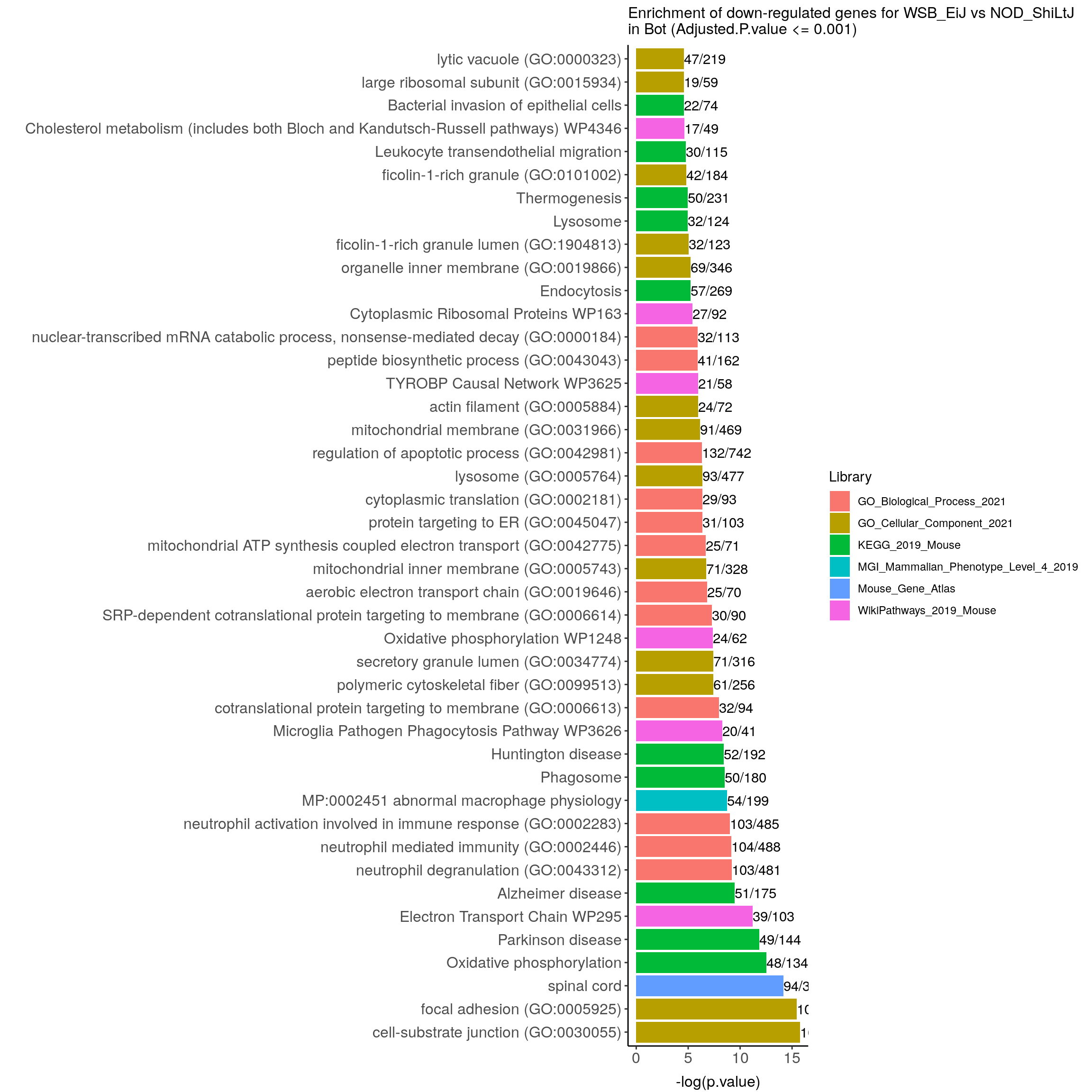
| Version | Author | Date |
|---|---|---|
| f6ccb3e | xhyuo | 2021-07-01 |
The effect of Strain in NTS with one outlier removed
#This is, by definition, the main effect plus the interaction term
#Building the results table
res.tab.strain.in.NTS <- results(res, list(c("Strain_WSB_EiJ_vs_NOD_ShiLtJ",
                                             "TissueNTS.StrainWSB_EiJ")), alpha = 0.05)
summary(res.tab.strain.in.NTS)
out of 27093 with nonzero total read count
adjusted p-value < 0.05
LFC > 0 (up) : 1713, 6.3%
LFC < 0 (down) : 2329, 8.6%
outliers [1] : 40, 0.15%
low counts [2] : 2620, 9.7%
(mean count < 1)
[1] see 'cooksCutoff' argument of ?results
[2] see 'independentFiltering' argument of ?resultstable(res.tab.strain.in.NTS$padj < 0.05)
FALSE TRUE
20391 4042 #We subset the results table to these genes and then sort it by the log2 fold change estimate to get the significant genes with the strongest down-regulation:
resSig.strain.in.NTS <- subset(res.tab.strain.in.NTS, padj < 0.05)
head(resSig.strain.in.NTS[order(resSig.strain.in.NTS$log2FoldChange), ])log2 fold change (MLE): Strain_WSB_EiJ_vs_NOD_ShiLtJ+TissueNTS.StrainWSB_EiJ effect
Wald test p-value: Strain_WSB_EiJ_vs_NOD_ShiLtJ+TissueNTS.StrainWSB_EiJ effect
DataFrame with 6 rows and 6 columns
baseMean log2FoldChange lfcSE stat pvalue
<numeric> <numeric> <numeric> <numeric> <numeric>
ENSMUSG00000020713 68.5623 -25.1959 3.445525 -7.31266 2.61914e-13
ENSMUSG00000092365 377.0809 -12.0428 0.921024 -13.07548 4.54714e-39
ENSMUSG00000053038 482.1118 -11.5790 0.933262 -12.40703 2.39367e-35
ENSMUSG00000079018 268.8942 -10.8340 0.928606 -11.66694 1.88061e-31
ENSMUSG00000066553 180.7374 -10.3833 0.921320 -11.27000 1.84564e-29
ENSMUSG00000101878 103.8932 -10.2895 0.936747 -10.98426 4.54952e-28
padj
<numeric>
ENSMUSG00000020713 1.67962e-11
ENSMUSG00000092365 1.27701e-36
ENSMUSG00000053038 5.90752e-33
ENSMUSG00000079018 3.82907e-29
ENSMUSG00000066553 3.31577e-27
ENSMUSG00000101878 7.77332e-26# with the strongest up-regulation:
head(resSig.strain.in.NTS[order(resSig.strain.in.NTS$log2FoldChange, decreasing = TRUE), ])log2 fold change (MLE): Strain_WSB_EiJ_vs_NOD_ShiLtJ+TissueNTS.StrainWSB_EiJ effect
Wald test p-value: Strain_WSB_EiJ_vs_NOD_ShiLtJ+TissueNTS.StrainWSB_EiJ effect
DataFrame with 6 rows and 6 columns
baseMean log2FoldChange lfcSE stat pvalue
<numeric> <numeric> <numeric> <numeric> <numeric>
ENSMUSG00000094306 2169.6074 13.17114 0.822877 16.0062 1.15649e-57
ENSMUSG00000094518 128.3642 10.52479 0.873274 12.0521 1.89040e-33
ENSMUSG00000103706 101.2714 10.13095 0.857331 11.8168 3.19445e-32
ENSMUSG00000096039 105.1752 10.08152 0.856462 11.7711 5.49909e-32
ENSMUSG00000021908 1516.5166 9.78597 0.325128 30.0988 5.02247e-199
ENSMUSG00000083773 39.8434 8.91494 0.876863 10.1669 2.78755e-24
padj
<numeric>
ENSMUSG00000094306 4.78925e-55
ENSMUSG00000094518 4.35737e-31
ENSMUSG00000103706 6.72844e-30
ENSMUSG00000096039 1.14837e-29
ENSMUSG00000021908 9.43955e-196
ENSMUSG00000083773 4.05406e-22#Visualization for res.tab.strain.in.NTS------
#Volcano plot
## Obtain logical vector regarding whether padj values are less than 0.05
threshold_OE <- (res.tab.strain.in.NTS$padj < 0.05 & !is.na(res.tab.strain.in.NTS$padj) & abs(res.tab.strain.in.NTS$log2FoldChange) >= 1)
## Determine the number of TRUE values
length(which(threshold_OE))[1] 1422## Add logical vector as a column (threshold) to the res.tab.strain.in.NTS
res.tab.strain.in.NTS$threshold <- threshold_OE
## Sort by ordered padj
res.tab.strain.in.NTS_ordered <- res.tab.strain.in.NTS %>%
data.frame() %>%
rownames_to_column(var="ENSEMBL") %>%
arrange(padj) %>%
mutate(genelabels = "") %>%
as_tibble() %>%
left_join(genes)Joining, by = "ENSEMBL"## Create a column to indicate which genes to label
res.tab.strain.in.NTS_ordered$genelabels[1:10] <- res.tab.strain.in.NTS_ordered$SYMBOL[1:10]
#display res.tab.strain.in.NTS_ordered
DT::datatable(res.tab.strain.in.NTS_ordered[(res.tab.strain.in.NTS_ordered$padj < 0.05 & !is.na(res.tab.strain.in.NTS_ordered$padj)), ],
filter = list(position = 'top', clear = FALSE),
extensions = 'Buttons',
options = list(dom = 'Blfrtip',
buttons = c('csv', 'excel'),
lengthMenu = list(c(10,25,50,-1),c(10,25,50,"All")),
pageLength = 40,
scrollY = "300px",
scrollX = "40px"),
caption = htmltools::tags$caption(style = 'caption-side: top; text-align: left; color:black; font-size:200% ;','DEG for WSB_EiJ vs NOD_ShiLtJ in NTS (fdr < 0.05)'))write.csv(res.tab.strain.in.NTS_ordered[(res.tab.strain.in.NTS_ordered$padj < 0.05 & !is.na(res.tab.strain.in.NTS_ordered$padj)), ],
file = "data/rnaseq/DEG_WSB_vs_NOD_in_NTS_fdr_0.05_with_one_outlier_removed.csv",
row.names = F, quote = F)
#Volcano plot
volcano.plot.strain.in.NTS <- ggplot(res.tab.strain.in.NTS_ordered) +
  geom_point(aes(x = log2FoldChange, y = -log10(padj), colour = threshold)) +
  scale_color_manual(values=c("blue", "red")) +
  geom_text_repel(aes(x = log2FoldChange, y = -log10(padj),
                      label = genelabels,
                      size = 3.5)) +
  ggtitle("DEG for WSB_EiJ vs NOD_ShiLtJ in NTS") +
  xlab("log2 fold change") +
  ylab("-log10 adjusted p-value") +
  theme(legend.position = "none",
        plot.title = element_text(size = rel(1.5), hjust = 0.5),
        axis.title = element_text(size = rel(1.25)))
print(volcano.plot.strain.in.NTS)
Warning: Removed 2662 rows containing missing values (geom_point).Warning: Removed 2665 rows containing missing values (geom_text_repel).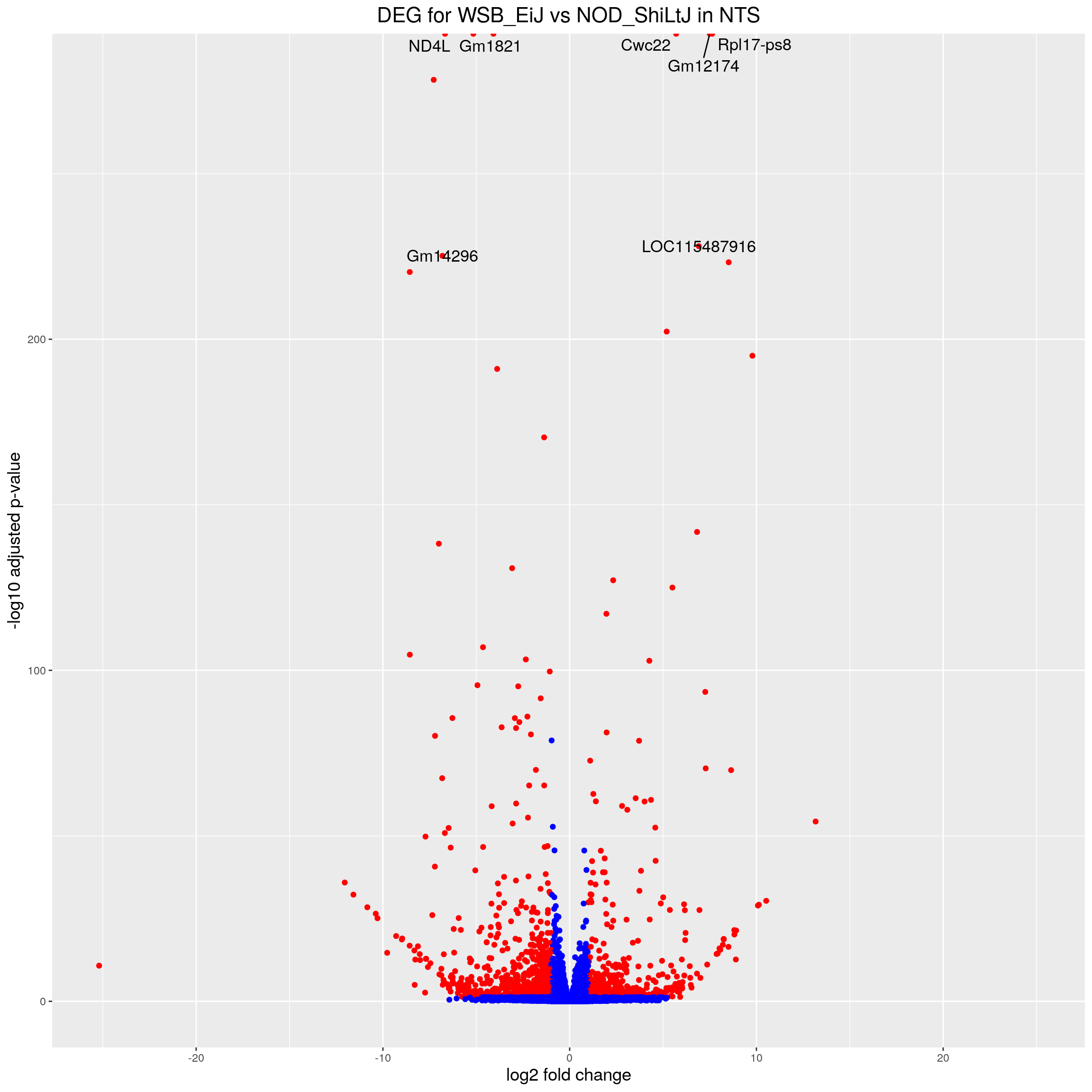
| Version | Author | Date |
|---|---|---|
| f6ccb3e | xhyuo | 2021-07-01 |
#heatmap
# Extract normalized expression for significant genes fdr < 0.05 & abs(log2FoldChange) >= 1)
normalized_counts_sig.strain.in.NTS <- normalized_counts %>%
filter(gene %in% rownames(subset(resSig.strain.in.NTS, padj < 0.05 & abs(log2FoldChange) >= 1))) %>%
dplyr::select(-1) %>%
dplyr::select(contains("NTS")) %>%
dplyr::select(-M6_WSB_EiJ_NTS)
### Set a color palette
heat_colors <- brewer.pal(6, "YlOrRd")
#annotation
df <- as.data.frame(colData(ddsMat)[,c("Strain","Tissue")]) %>%
filter(Tissue == "NTS") %>%
filter(rownames(.) != "M6_WSB_EiJ_NTS")
### Run pheatmap using the metadata data frame for the annotation
sig.strain.in.NTS.plot <- pheatmap(as.matrix(normalized_counts_sig.strain.in.NTS),
color = heat_colors,
cluster_rows = T,
show_rownames = F,
annotation_col = df,
annotation_colors = list(Strain = c(NOD_ShiLtJ = "#0064C9",
WSB_EiJ ="#B10DC9"),
Tissue = c(Bot = "#96ca00",
NTS = "#ff9289")),
border_color = NA,
fontsize = 10,
scale = "row",
fontsize_row = 10,
height = 20 #legend = FALSE, annotation_legend = FALSE, annotation_names_col = FALSE,
#main = "Heatmap of the top DEGs in WSB_EiJ vs NOD_ShiLtJ in NTS (fdr < 0.05 & abs(log2FoldChange) >= 1)"
)
sig.strain.in.NTS.plot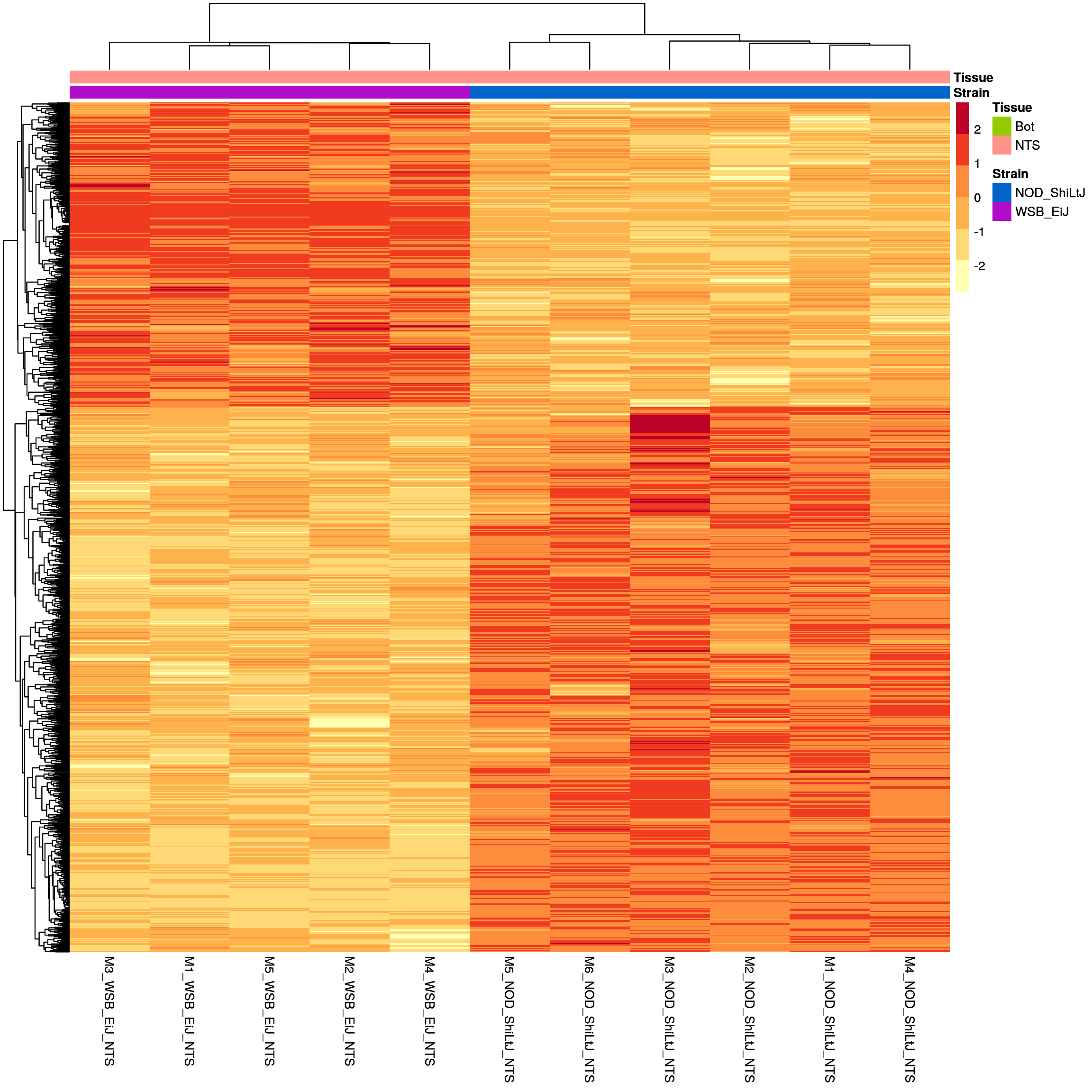
| Version | Author | Date |
|---|---|---|
| f6ccb3e | xhyuo | 2021-07-01 |
#plot sig.strain.in.Bot.plot and sig.strain.in.NTS.plot together-------
ht.map2.plot = plot_grid(as.grob(sig.strain.in.Bot.plot),
          as.grob(sig.strain.in.NTS.plot),
          align = "h", rel_widths = c(1, 1.3),
          labels = c('A', 'B'))
#add title
# now add the title
title <- ggdraw() +
  draw_label(
    "Heatmap of the top DEGs in WSB_EiJ vs NOD_ShiLtJ in Bot and NTS, respectively (fdr < 0.05 & abs(log2FoldChange) >= 1)",
    fontface = 'bold',
    x = 0,
    hjust = 0
  )
plot_grid(
  title,
  ht.map2.plot,
  ncol = 1,
  # rel_heights values control vertical title margins
  rel_heights = c(0.1, 1)
)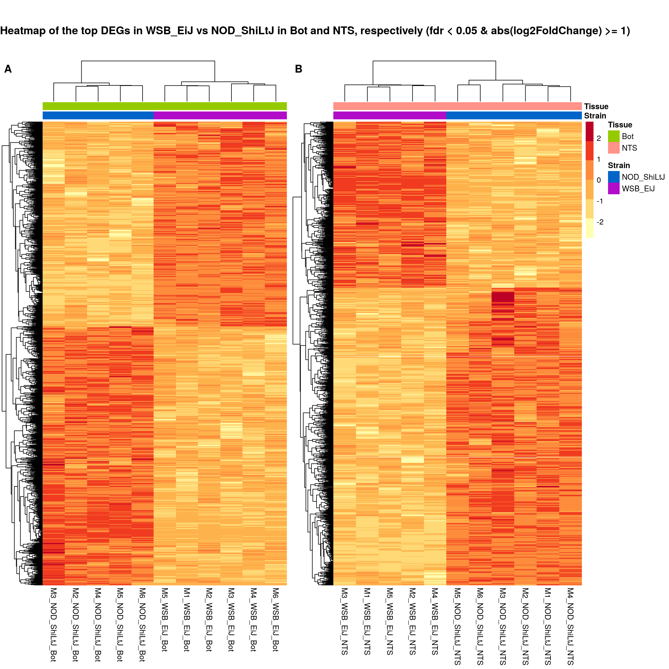
| Version | Author | Date |
|---|---|---|
| f6ccb3e | xhyuo | 2021-07-01 |
#logFC heatmap on both Bot and NTS top DEGs-----
restop.tab.in.Bot.NTS <- full_join(res.tab.strain.in.Bot_ordered,
                                   res.tab.strain.in.NTS_ordered,
                                   by = c("ENSEMBL", "SYMBOL")) %>%
  filter((ENSEMBL %in% res.tab.strain.in.Bot_ordered$ENSEMBL[1:30]) | (ENSEMBL %in% res.tab.strain.in.NTS_ordered$ENSEMBL[1:30]))

restop.tab.in.Bot.NTS.mat <- as.matrix(restop.tab.in.Bot.NTS[, c("log2FoldChange.x", "log2FoldChange.y")])
rownames(restop.tab.in.Bot.NTS.mat) <-
  ifelse(is.na(restop.tab.in.Bot.NTS$SYMBOL),
         restop.tab.in.Bot.NTS$ENSEMBL,
         paste0(restop.tab.in.Bot.NTS$SYMBOL,":", restop.tab.in.Bot.NTS$ENSEMBL))
colnames(restop.tab.in.Bot.NTS.mat) <- c("Bot", "NTS")

#heatmap
### Run pheatmap using the metadata data frame for the annotation
pheatmap(restop.tab.in.Bot.NTS.mat,
         color = colorpanel(1000, "blue", "white", "red"),
         cluster_rows  = T,
         show_rownames = T,
         border_color  = NA,
         fontsize = 10,
         fontsize_row = 8,
         height = 25,
         main = "Heatmap of log2FoldChange for the top 30 DEGs in Bot and NTS")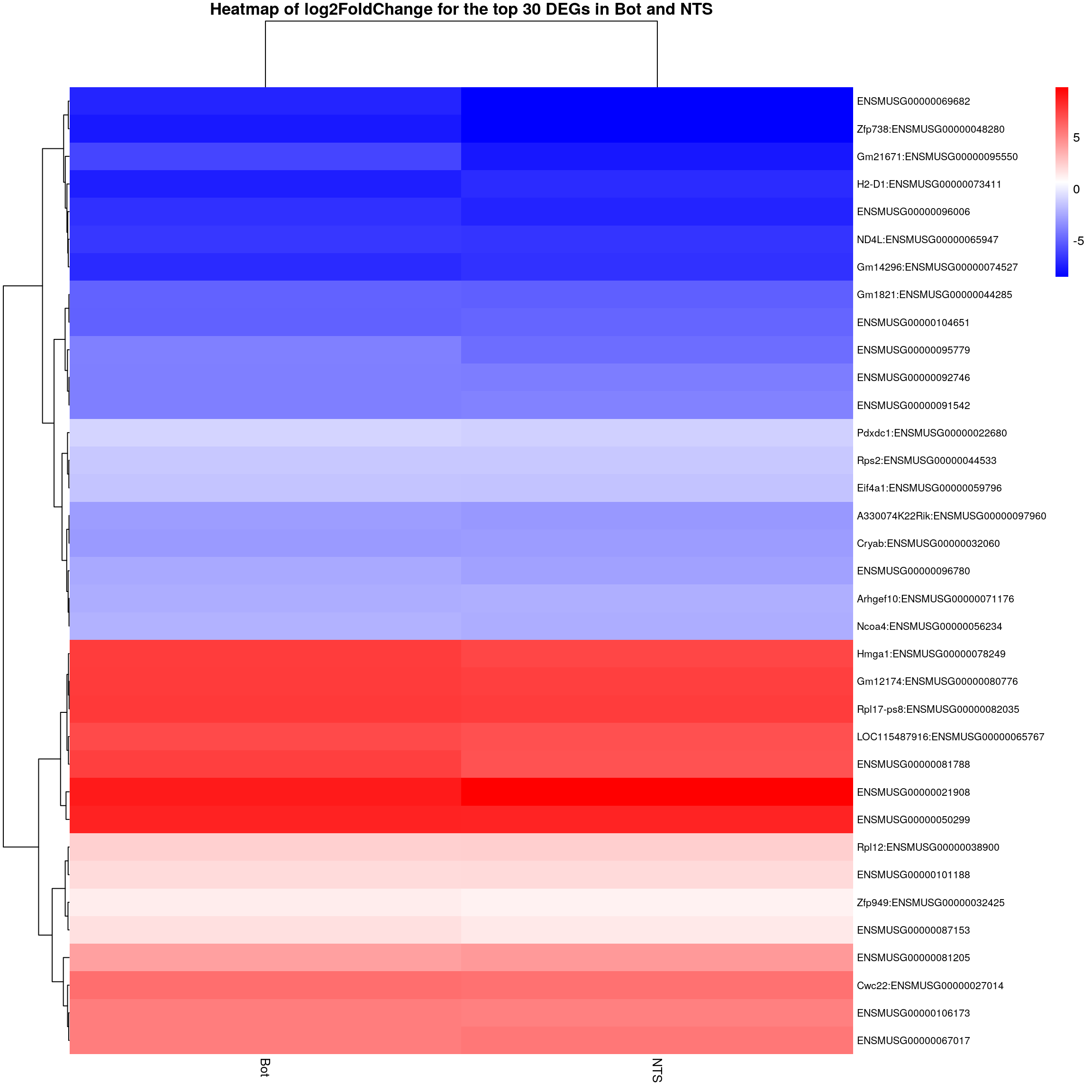
| Version | Author | Date |
|---|---|---|
| f6ccb3e | xhyuo | 2021-07-01 |
#enrichment analysis for res.tab.strain.in.NTS-------
dbs <- c("WikiPathways_2019_Mouse",
         "GO_Biological_Process_2021",
         "GO_Cellular_Component_2021",
         "GO_Molecular_Function_2021",
         "KEGG_2019_Mouse",
         "Mouse_Gene_Atlas",
         "MGI_Mammalian_Phenotype_Level_4_2019")

#results (fdr < 0.05)------
resSig.strain.in.NTS.tab <- resSig.strain.in.NTS %>%
  data.frame() %>%
  rownames_to_column(var="ENSEMBL") %>%
  as_tibble() %>%
  left_join(genes)
Joining, by = "ENSEMBL"#up-regulated genes WSB_EiJ vs NOD_ShiLtJ in NTS ---------------------------
up.genes <- resSig.strain.in.NTS.tab %>%
filter(log2FoldChange > 0) %>%
pull(SYMBOL)
#up-regulated genes enrichment
up.genes.enriched <- enrichr(as.character(na.omit(up.genes)), dbs)Uploading data to Enrichr... Done.
Querying WikiPathways_2019_Mouse... Done.
Querying GO_Biological_Process_2021... Done.
Querying GO_Cellular_Component_2021... Done.
Querying GO_Molecular_Function_2021... Done.
Querying KEGG_2019_Mouse... Done.
Querying Mouse_Gene_Atlas... Done.
Querying MGI_Mammalian_Phenotype_Level_4_2019... Done.
Parsing results... Done.for (j in 1:length(up.genes.enriched)){
up.genes.enriched[[j]] <- cbind(data.frame(Library = names(up.genes.enriched)[j]),up.genes.enriched[[j]])
}
up.genes.enriched <- do.call(rbind.data.frame, up.genes.enriched) %>%
filter(Adjusted.P.value <= 0.2) %>%
mutate(logpvalue = -log10(P.value)) %>%
arrange(desc(logpvalue))
#display up.genes.enriched
DT::datatable(up.genes.enriched,
filter = list(position = 'top', clear = FALSE),
extensions = 'Buttons',
options = list(dom = 'Blfrtip',
buttons = c('csv', 'excel'),
lengthMenu = list(c(10,25,50,-1),c(10,25,50,"All")),
pageLength = 40,
scrollY = "300px",
scrollX = "40px")
)#barpot
up.genes.enriched.plot.in.NTS <- up.genes.enriched %>%
filter(Adjusted.P.value <= 0.2) %>%
mutate(Term = fct_reorder(Term, -logpvalue)) %>%
ggplot(data = ., aes(x = Term, y = logpvalue, fill = Library, label = Overlap)) +
geom_bar(stat = "identity") +
geom_text(position = position_dodge(width = 0.9),
hjust = 0) +
theme_bw() +
ylab("-log(p.value)") +
xlab("") +
ggtitle("Enrichment of up-regulated genes for WSB_EiJ vs NOD_ShiLtJ \nin NTS (Adjusted.P.value <= 0.2)") +
theme(plot.background = element_blank() ,
panel.border = element_blank(),
panel.background = element_blank(),
#legend.position = "none",
plot.title = element_text(hjust = 0),
panel.grid.major = element_blank(),
panel.grid.minor = element_blank()) +
theme(axis.line = element_line(color = 'black')) +
theme(axis.title.x = element_text(size = 12, vjust=-0.5)) +
theme(axis.title.y = element_text(size = 12, vjust= 1.0)) +
theme(axis.text = element_text(size = 12)) +
theme(plot.title = element_text(size = 12)) +
coord_flip()
up.genes.enriched.plot.in.NTS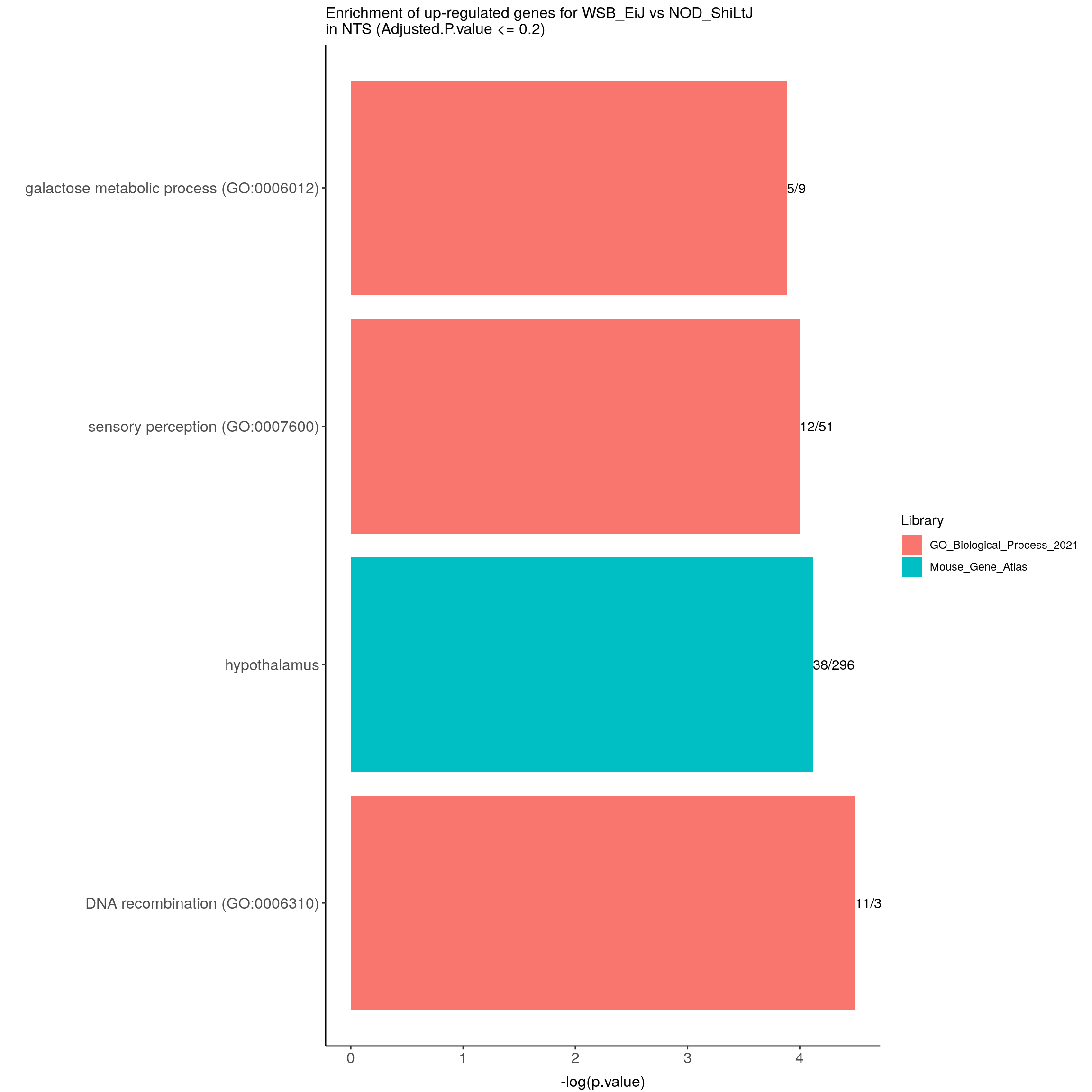
| Version | Author | Date |
|---|---|---|
| f6ccb3e | xhyuo | 2021-07-01 |
#down-regulated genes WSB_EiJ vs NOD_ShiLtJ in NTS---------------------------
down.genes <- resSig.strain.in.NTS.tab %>%
  filter(log2FoldChange < 0) %>%
  pull(SYMBOL)
#down-regulated genes enrichment
down.genes.enriched <- enrichr(as.character(na.omit(down.genes)), dbs)
Uploading data to Enrichr... Done.
Querying WikiPathways_2019_Mouse... Done.
Querying GO_Biological_Process_2021... Done.
Querying GO_Cellular_Component_2021... Done.
Querying GO_Molecular_Function_2021... Done.
Querying KEGG_2019_Mouse... Done.
Querying Mouse_Gene_Atlas... Done.
Querying MGI_Mammalian_Phenotype_Level_4_2019... Done.
Parsing results... Done.for (j in 1:length(down.genes.enriched)){
down.genes.enriched[[j]] <- cbind(data.frame(Library = names(down.genes.enriched)[j]),down.genes.enriched[[j]])
}
down.genes.enriched <- do.call(rbind.data.frame, down.genes.enriched) %>%
filter(Adjusted.P.value <= 0.05) %>%
mutate(logpvalue = -log10(P.value)) %>%
arrange(desc(logpvalue))
#display down.genes.enriched
DT::datatable(down.genes.enriched,
filter = list(position = 'top', clear = FALSE),
extensions = 'Buttons',
options = list(dom = 'Blfrtip',
buttons = c('csv', 'excel'),
lengthMenu = list(c(10,25,50,-1),c(10,25,50,"All")),
pageLength = 40,
scrollY = "300px",
scrollX = "40px")
)#barpot
down.genes.enriched.plot.in.NTS <- down.genes.enriched %>%
filter(Adjusted.P.value <= 0.001) %>%
mutate(Term = fct_reorder(Term, -logpvalue)) %>%
ggplot(data = ., aes(x = Term, y = logpvalue, fill = Library, label = Overlap)) +
geom_bar(stat = "identity") +
geom_text(position = position_dodge(width = 0.9),
hjust = 0) +
theme_bw() +
ylab("-log(p.value)") +
xlab("") +
ggtitle("Enrichment of down-regulated genes for WSB_EiJ vs NOD_ShiLtJ \nin NTS (Adjusted.P.value <= 0.001)") +
theme(plot.background = element_blank() ,
panel.border = element_blank(),
panel.background = element_blank(),
#legend.position = "none",
plot.title = element_text(hjust = 0),
panel.grid.major = element_blank(),
panel.grid.minor = element_blank()) +
theme(axis.line = element_line(color = 'black')) +
theme(axis.title.x = element_text(size = 12, vjust=-0.5)) +
theme(axis.title.y = element_text(size = 12, vjust= 1.0)) +
theme(axis.text = element_text(size = 12)) +
theme(plot.title = element_text(size = 12)) +
coord_flip()
down.genes.enriched.plot.in.NTS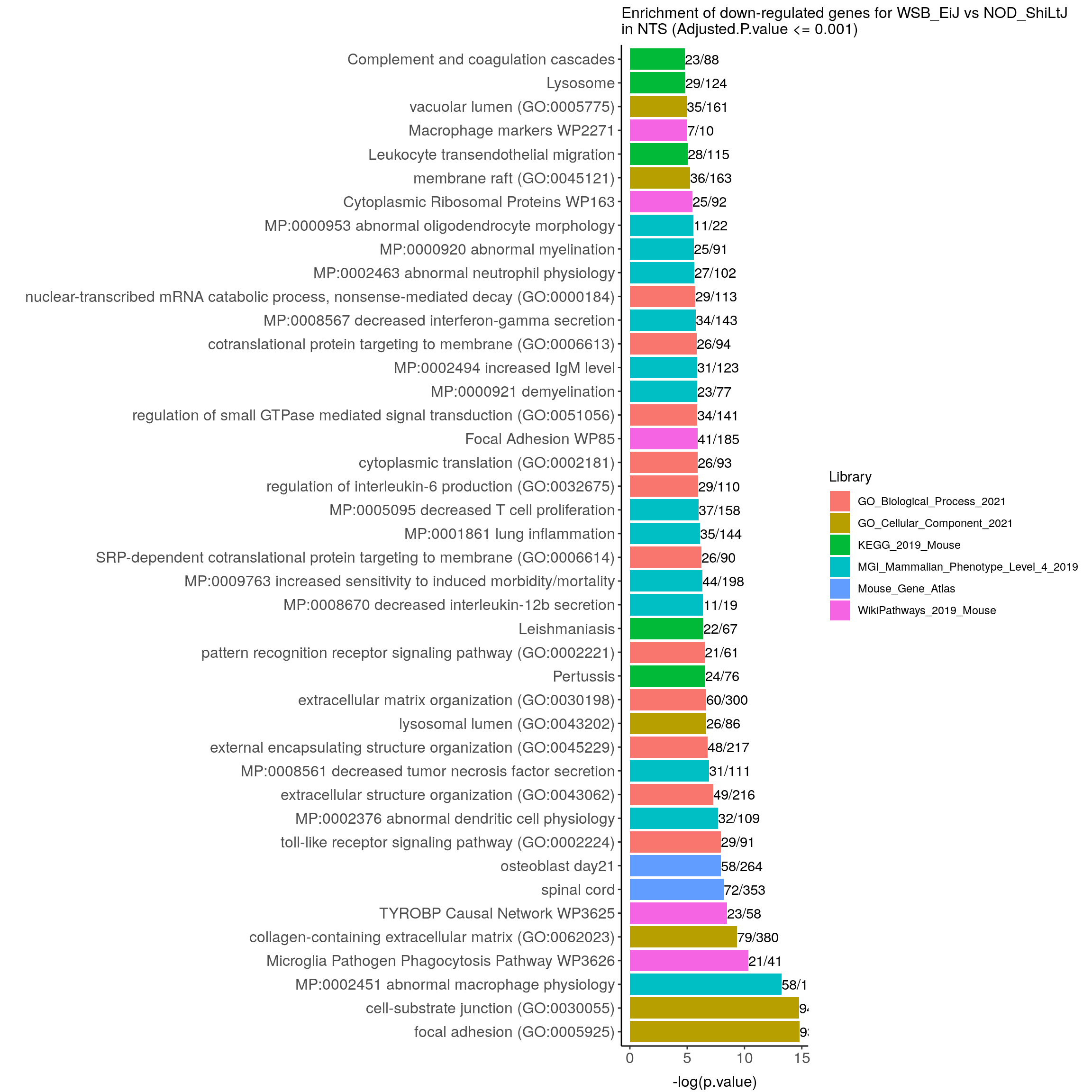
| Version | Author | Date |
|---|---|---|
| f6ccb3e | xhyuo | 2021-07-01 |
sessionInfo()R version 4.0.3 (2020-10-10)
Platform: x86_64-pc-linux-gnu (64-bit)
Running under: Ubuntu 20.04.1 LTS
Matrix products: default
BLAS/LAPACK: /usr/lib/x86_64-linux-gnu/openblas-pthread/libopenblasp-r0.3.8.so
locale:
[1] LC_CTYPE=en_US.UTF-8 LC_NUMERIC=C
[3] LC_TIME=en_US.UTF-8 LC_COLLATE=en_US.UTF-8
[5] LC_MONETARY=en_US.UTF-8 LC_MESSAGES=C
[7] LC_PAPER=en_US.UTF-8 LC_NAME=C
[9] LC_ADDRESS=C LC_TELEPHONE=C
[11] LC_MEASUREMENT=en_US.UTF-8 LC_IDENTIFICATION=C
attached base packages:
[1] parallel stats4 stats graphics grDevices utils datasets
[8] methods base
other attached packages:
[1] ggplotify_0.0.7 cowplot_1.1.1
[3] enrichR_3.0 DT_0.17
[5] ggrepel_0.9.0 pheatmap_1.0.12
[7] DESeq2_1.30.1 SummarizedExperiment_1.18.2
[9] DelayedArray_0.14.1 matrixStats_0.57.0
[11] GenomicRanges_1.40.0 GenomeInfoDb_1.26.2
[13] RColorBrewer_1.1-2 org.Mm.eg.db_3.11.4
[15] AnnotationDbi_1.52.0 IRanges_2.22.2
[17] S4Vectors_0.26.1 Biobase_2.48.0
[19] BiocGenerics_0.36.0 gplots_3.1.1
[21] Glimma_2.0.0 edgeR_3.32.1
[23] limma_3.46.0 forcats_0.5.0
[25] dplyr_1.0.2 purrr_0.3.4
[27] readr_1.4.0 tidyr_1.1.2
[29] tibble_3.0.4 ggplot2_3.3.3
[31] tidyverse_1.3.0 stringr_1.4.0
[33] workflowr_1.6.2
loaded via a namespace (and not attached):
[1] colorspace_2.0-0 rjson_0.2.20 ellipsis_0.3.1
[4] rprojroot_2.0.2 XVector_0.28.0 fs_1.5.0
[7] rstudioapi_0.13 farver_2.0.3 bit64_4.0.5
[10] fansi_0.4.1 lubridate_1.7.9.2 xml2_1.3.2
[13] splines_4.0.3 geneplotter_1.66.0 knitr_1.30
[16] jsonlite_1.7.2 broom_0.7.3 annotate_1.66.0
[19] dbplyr_2.0.0 BiocManager_1.30.10 compiler_4.0.3
[22] httr_1.4.2 rvcheck_0.1.8 backports_1.2.1
[25] assertthat_0.2.1 Matrix_1.3-2 cli_2.2.0
[28] later_1.1.0.1 htmltools_0.5.1 tools_4.0.3
[31] gtable_0.3.0 glue_1.4.2 GenomeInfoDbData_1.2.4
[34] Rcpp_1.0.5 cellranger_1.1.0 vctrs_0.3.6
[37] crosstalk_1.1.1 xfun_0.20 rvest_0.3.6
[40] lifecycle_0.2.0 gtools_3.8.2 XML_3.99-0.5
[43] zlibbioc_1.36.0 scales_1.1.1 hms_1.0.0
[46] promises_1.1.1 curl_4.3 yaml_2.2.1
[49] memoise_1.1.0 stringi_1.5.3 RSQLite_2.2.2
[52] genefilter_1.70.0 caTools_1.18.1 BiocParallel_1.22.0
[55] rlang_0.4.10 pkgconfig_2.0.3 bitops_1.0-6
[58] evaluate_0.14 lattice_0.20-41 labeling_0.4.2
[61] htmlwidgets_1.5.3 bit_4.0.4 tidyselect_1.1.0
[64] magrittr_2.0.1 R6_2.5.0 generics_0.1.0
[67] DBI_1.1.0 pillar_1.4.7 haven_2.3.1
[70] whisker_0.4 withr_2.3.0 survival_3.2-7
[73] RCurl_1.98-1.2 modelr_0.1.8 crayon_1.3.4
[76] KernSmooth_2.23-18 rmarkdown_2.6 locfit_1.5-9.4
[79] grid_4.0.3 readxl_1.3.1 blob_1.2.1
[82] git2r_0.28.0 reprex_0.3.0 digest_0.6.27
[85] xtable_1.8-4 httpuv_1.5.5 gridGraphics_0.5-1
[88] munsell_0.5.0 This R Markdown site was created with workflowr