DEG_analysis_on_ transcript
Last updated: 2021-08-10
Checks: 6 1
Knit directory: DO_Opioid/
This reproducible R Markdown analysis was created with workflowr (version 1.6.2). The Checks tab describes the reproducibility checks that were applied when the results were created. The Past versions tab lists the development history.
Great! Since the R Markdown file has been committed to the Git repository, you know the exact version of the code that produced these results.
Great job! The global environment was empty. Objects defined in the global environment can affect the analysis in your R Markdown file in unknown ways. For reproduciblity it’s best to always run the code in an empty environment.
The command set.seed(20200504) was run prior to running the code in the R Markdown file. Setting a seed ensures that any results that rely on randomness, e.g. subsampling or permutations, are reproducible.
Great job! Recording the operating system, R version, and package versions is critical for reproducibility.
Nice! There were no cached chunks for this analysis, so you can be confident that you successfully produced the results during this run.
Using absolute paths to the files within your workflowr project makes it difficult for you and others to run your code on a different machine. Change the absolute path(s) below to the suggested relative path(s) to make your code more reproducible.
| absolute | relative |
|---|---|
| /projects/compsci/USERS/heh/DO_Opioid/data/rnaseq/merged.dgerc.isoforms.csv | data/rnaseq/merged.dgerc.isoforms.csv |
| /projects/compsci/USERS/heh/DO_Opioid/data/rnaseq/merged.dgerc.isoforms.RData | data/rnaseq/merged.dgerc.isoforms.RData |
Great! You are using Git for version control. Tracking code development and connecting the code version to the results is critical for reproducibility.
The results in this page were generated with repository version a242947. See the Past versions tab to see a history of the changes made to the R Markdown and HTML files.
Note that you need to be careful to ensure that all relevant files for the analysis have been committed to Git prior to generating the results (you can use wflow_publish or wflow_git_commit). workflowr only checks the R Markdown file, but you know if there are other scripts or data files that it depends on. Below is the status of the Git repository when the results were generated:
Ignored files:
    Ignored:    .RData
    Ignored:    .Rhistory
    Ignored:    .Rproj.user/
    Ignored:    analysis/Picture1.png
    Ignored:    data/output/

Untracked files:
    Untracked:  analysis/DDO_morphine1_second_set_69k.stdout
    Untracked:  analysis/DO_morphine1.R
    Untracked:  analysis/DO_morphine1.Rout
    Untracked:  analysis/DO_morphine1.sh
    Untracked:  analysis/DO_morphine1.stderr
    Untracked:  analysis/DO_morphine1.stdout
    Untracked:  analysis/DO_morphine1_SNP.R
    Untracked:  analysis/DO_morphine1_SNP.Rout
    Untracked:  analysis/DO_morphine1_SNP.sh
    Untracked:  analysis/DO_morphine1_SNP.stderr
    Untracked:  analysis/DO_morphine1_SNP.stdout
    Untracked:  analysis/DO_morphine1_combined.R
    Untracked:  analysis/DO_morphine1_combined.Rout
    Untracked:  analysis/DO_morphine1_combined.sh
    Untracked:  analysis/DO_morphine1_combined.stderr
    Untracked:  analysis/DO_morphine1_combined.stdout
    Untracked:  analysis/DO_morphine1_combined_69k.R
    Untracked:  analysis/DO_morphine1_combined_69k.Rout
    Untracked:  analysis/DO_morphine1_combined_69k.sh
    Untracked:  analysis/DO_morphine1_combined_69k.stderr
    Untracked:  analysis/DO_morphine1_combined_69k.stdout
    Untracked:  analysis/DO_morphine1_combined_69k_m2.R
    Untracked:  analysis/DO_morphine1_combined_69k_m2.Rout
    Untracked:  analysis/DO_morphine1_combined_69k_m2.sh
    Untracked:  analysis/DO_morphine1_combined_69k_m2.stderr
    Untracked:  analysis/DO_morphine1_combined_69k_m2.stdout
    Untracked:  analysis/DO_morphine1_combined_weight_DOB.R
    Untracked:  analysis/DO_morphine1_combined_weight_DOB.Rout
    Untracked:  analysis/DO_morphine1_combined_weight_DOB.err
    Untracked:  analysis/DO_morphine1_combined_weight_DOB.out
    Untracked:  analysis/DO_morphine1_combined_weight_DOB.sh
    Untracked:  analysis/DO_morphine1_combined_weight_DOB.stderr
    Untracked:  analysis/DO_morphine1_combined_weight_DOB.stdout
    Untracked:  analysis/DO_morphine1_combined_weight_age.R
    Untracked:  analysis/DO_morphine1_combined_weight_age.err
    Untracked:  analysis/DO_morphine1_combined_weight_age.out
    Untracked:  analysis/DO_morphine1_combined_weight_age.sh
    Untracked:  analysis/DO_morphine1_combined_weight_age_GAMMT.R
    Untracked:  analysis/DO_morphine1_combined_weight_age_GAMMT.err
    Untracked:  analysis/DO_morphine1_combined_weight_age_GAMMT.out
    Untracked:  analysis/DO_morphine1_combined_weight_age_GAMMT.sh
    Untracked:  analysis/DO_morphine1_combined_weight_age_GAMMT_chr19.R
    Untracked:  analysis/DO_morphine1_combined_weight_age_GAMMT_chr19.err
    Untracked:  analysis/DO_morphine1_combined_weight_age_GAMMT_chr19.out
    Untracked:  analysis/DO_morphine1_combined_weight_age_GAMMT_chr19.sh
    Untracked:  analysis/DO_morphine1_cph.R
    Untracked:  analysis/DO_morphine1_cph.Rout
    Untracked:  analysis/DO_morphine1_cph.sh
    Untracked:  analysis/DO_morphine1_second_set.R
    Untracked:  analysis/DO_morphine1_second_set.Rout
    Untracked:  analysis/DO_morphine1_second_set.sh
    Untracked:  analysis/DO_morphine1_second_set.stderr
    Untracked:  analysis/DO_morphine1_second_set.stdout
    Untracked:  analysis/DO_morphine1_second_set_69k.R
    Untracked:  analysis/DO_morphine1_second_set_69k.Rout
    Untracked:  analysis/DO_morphine1_second_set_69k.sh
    Untracked:  analysis/DO_morphine1_second_set_69k.stderr
    Untracked:  analysis/DO_morphine1_second_set_SNP.R
    Untracked:  analysis/DO_morphine1_second_set_SNP.Rout
    Untracked:  analysis/DO_morphine1_second_set_SNP.sh
    Untracked:  analysis/DO_morphine1_second_set_SNP.stderr
    Untracked:  analysis/DO_morphine1_second_set_SNP.stdout
    Untracked:  analysis/DO_morphine1_second_set_weight_DOB.R
    Untracked:  analysis/DO_morphine1_second_set_weight_DOB.Rout
    Untracked:  analysis/DO_morphine1_second_set_weight_DOB.err
    Untracked:  analysis/DO_morphine1_second_set_weight_DOB.out
    Untracked:  analysis/DO_morphine1_second_set_weight_DOB.sh
    Untracked:  analysis/DO_morphine1_second_set_weight_DOB.stderr
    Untracked:  analysis/DO_morphine1_second_set_weight_DOB.stdout
    Untracked:  analysis/DO_morphine1_second_set_weight_age.R
    Untracked:  analysis/DO_morphine1_second_set_weight_age.Rout
    Untracked:  analysis/DO_morphine1_second_set_weight_age.err
    Untracked:  analysis/DO_morphine1_second_set_weight_age.out
    Untracked:  analysis/DO_morphine1_second_set_weight_age.sh
    Untracked:  analysis/DO_morphine1_second_set_weight_age.stderr
    Untracked:  analysis/DO_morphine1_second_set_weight_age.stdout
    Untracked:  analysis/DO_morphine1_weight_DOB.R
    Untracked:  analysis/DO_morphine1_weight_DOB.sh
    Untracked:  analysis/DO_morphine1_weight_age.R
    Untracked:  analysis/DO_morphine1_weight_age.sh
    Untracked:  analysis/DO_morphine_gemma.R
    Untracked:  analysis/DO_morphine_gemma.err
    Untracked:  analysis/DO_morphine_gemma.out
    Untracked:  analysis/DO_morphine_gemma.sh
    Untracked:  analysis/DO_morphine_gemma_firstmin.R
    Untracked:  analysis/DO_morphine_gemma_firstmin.err
    Untracked:  analysis/DO_morphine_gemma_firstmin.out
    Untracked:  analysis/DO_morphine_gemma_firstmin.sh
    Untracked:  analysis/DO_morphine_gemma_withpermu.R
    Untracked:  analysis/DO_morphine_gemma_withpermu.err
    Untracked:  analysis/DO_morphine_gemma_withpermu.out
    Untracked:  analysis/DO_morphine_gemma_withpermu.sh
    Untracked:  analysis/DO_morphine_gemma_withpermu_firstbatch_min.depression.R
    Untracked:  analysis/DO_morphine_gemma_withpermu_firstbatch_min.depression.err
    Untracked:  analysis/DO_morphine_gemma_withpermu_firstbatch_min.depression.out
    Untracked:  analysis/DO_morphine_gemma_withpermu_firstbatch_min.depression.sh
    Untracked:  analysis/Plot_DO_morphine1_SNP.R
    Untracked:  analysis/Plot_DO_morphine1_SNP.Rout
    Untracked:  analysis/Plot_DO_morphine1_SNP.sh
    Untracked:  analysis/Plot_DO_morphine1_SNP.stderr
    Untracked:  analysis/Plot_DO_morphine1_SNP.stdout
    Untracked:  analysis/Plot_DO_morphine1_second_set_SNP.R
    Untracked:  analysis/Plot_DO_morphine1_second_set_SNP.Rout
    Untracked:  analysis/Plot_DO_morphine1_second_set_SNP.sh
    Untracked:  analysis/Plot_DO_morphine1_second_set_SNP.stderr
    Untracked:  analysis/Plot_DO_morphine1_second_set_SNP.stdout
    Untracked:  analysis/scripts/
    Untracked:  analysis/workflow_proc.R
    Untracked:  analysis/workflow_proc.sh
    Untracked:  analysis/workflow_proc.stderr
    Untracked:  analysis/workflow_proc.stdout
    Untracked:  analysis/x.R
    Untracked:  code/cfw/
    Untracked:  code/gemma_plot.R
    Untracked:  code/reconst_utils.R
    Untracked:  data/69k_grid_pgmap.RData
    Untracked:  data/FinalReport/
    Untracked:  data/GM/
    Untracked:  data/GM_covar.csv
    Untracked:  data/GM_covar_07092018_morphine.csv
    Untracked:  data/Jackson_Lab_Bubier_MURGIGV01/
    Untracked:  data/MasterMorphine Second Set DO w DOB2.xlsx
    Untracked:  data/MasterMorphine Second Set DO.xlsx
    Untracked:  data/cc_variants.sqlite
    Untracked:  data/combined/
    Untracked:  data/first/
    Untracked:  data/founder_geno.csv
    Untracked:  data/genetic_map.csv
    Untracked:  data/gm.json
    Untracked:  data/gwas.sh
    Untracked:  data/marker_grid_0.02cM_plus.txt
    Untracked:  data/mouse_genes_mgi.sqlite
    Untracked:  data/pheno.csv
    Untracked:  data/pheno_qtl2.csv
    Untracked:  data/pheno_qtl2_07092018_morphine.csv
    Untracked:  data/pheno_qtl2_w_dob.csv
    Untracked:  data/physical_map.csv
    Untracked:  data/rnaseq/
    Untracked:  data/sample_geno.csv
    Untracked:  data/second/
    Untracked:  figure/
    Untracked:  glimma-plots/
    Untracked:  output/DO_morphine_Min.depression.png
    Untracked:  output/DO_morphine_Min.depression22222_violin_chr5.pdf
    Untracked:  output/DO_morphine_Min.depression_coefplot.pdf
    Untracked:  output/DO_morphine_Min.depression_coefplot_blup.pdf
    Untracked:  output/DO_morphine_Min.depression_coefplot_blup_chr5.png
    Untracked:  output/DO_morphine_Min.depression_coefplot_blup_chrX.png
    Untracked:  output/DO_morphine_Min.depression_coefplot_chr5.png
    Untracked:  output/DO_morphine_Min.depression_coefplot_chrX.png
    Untracked:  output/DO_morphine_Min.depression_peak_genes_chr5.png
    Untracked:  output/DO_morphine_Min.depression_violin_chr5.png
    Untracked:  output/DO_morphine_Recovery.Time.png
    Untracked:  output/DO_morphine_Recovery.Time_coefplot.pdf
    Untracked:  output/DO_morphine_Recovery.Time_coefplot_blup.pdf
    Untracked:  output/DO_morphine_Recovery.Time_coefplot_blup_chr11.png
    Untracked:  output/DO_morphine_Recovery.Time_coefplot_blup_chr4.png
    Untracked:  output/DO_morphine_Recovery.Time_coefplot_blup_chr7.png
    Untracked:  output/DO_morphine_Recovery.Time_coefplot_blup_chr9.png
    Untracked:  output/DO_morphine_Recovery.Time_coefplot_chr11.png
    Untracked:  output/DO_morphine_Recovery.Time_coefplot_chr4.png
    Untracked:  output/DO_morphine_Recovery.Time_coefplot_chr7.png
    Untracked:  output/DO_morphine_Recovery.Time_coefplot_chr9.png
    Untracked:  output/DO_morphine_Status_bin.png
    Untracked:  output/DO_morphine_Status_bin_coefplot.pdf
    Untracked:  output/DO_morphine_Status_bin_coefplot_blup.pdf
    Untracked:  output/DO_morphine_Survival.Time.png
    Untracked:  output/DO_morphine_Survival.Time_coefplot.pdf
    Untracked:  output/DO_morphine_Survival.Time_coefplot_blup.pdf
    Untracked:  output/DO_morphine_Survival.Time_coefplot_blup_chr17.png
    Untracked:  output/DO_morphine_Survival.Time_coefplot_blup_chr8.png
    Untracked:  output/DO_morphine_Survival.Time_coefplot_chr17.png
    Untracked:  output/DO_morphine_Survival.Time_coefplot_chr8.png
    Untracked:  output/DO_morphine_combine_batch_peak_violin.pdf
    Untracked:  output/DO_morphine_combined_69k_m2_Min.depression.png
    Untracked:  output/DO_morphine_combined_69k_m2_Min.depression_coefplot.pdf
    Untracked:  output/DO_morphine_combined_69k_m2_Min.depression_coefplot_blup.pdf
    Untracked:  output/DO_morphine_combined_69k_m2_Recovery.Time.png
    Untracked:  output/DO_morphine_combined_69k_m2_Recovery.Time_coefplot.pdf
    Untracked:  output/DO_morphine_combined_69k_m2_Recovery.Time_coefplot_blup.pdf
    Untracked:  output/DO_morphine_combined_69k_m2_Status_bin.png
    Untracked:  output/DO_morphine_combined_69k_m2_Status_bin_coefplot.pdf
    Untracked:  output/DO_morphine_combined_69k_m2_Status_bin_coefplot_blup.pdf
    Untracked:  output/DO_morphine_combined_69k_m2_Survival.Time.png
    Untracked:  output/DO_morphine_combined_69k_m2_Survival.Time_coefplot.pdf
    Untracked:  output/DO_morphine_combined_69k_m2_Survival.Time_coefplot_blup.pdf
    Untracked:  output/DO_morphine_coxph_24hrs_kinship_QTL.png
    Untracked:  output/DO_morphine_cphout.RData
    Untracked:  output/DO_morphine_first_batch_peak_in_second_batch_violin.pdf
    Untracked:  output/DO_morphine_first_batch_peak_in_second_batch_violin_sidebyside.pdf
    Untracked:  output/DO_morphine_first_batch_peak_violin.pdf
    Untracked:  output/DO_morphine_operm.cph.RData
    Untracked:  output/DO_morphine_second_batch_on_first_batch_peak_violin.pdf
    Untracked:  output/DO_morphine_second_batch_peak_ch6surv_on_first_batchviolin.pdf
    Untracked:  output/DO_morphine_second_batch_peak_ch6surv_on_first_batchviolin2.pdf
    Untracked:  output/DO_morphine_second_batch_peak_in_first_batch_violin.pdf
    Untracked:  output/DO_morphine_second_batch_peak_in_first_batch_violin_sidebyside.pdf
    Untracked:  output/DO_morphine_second_batch_peak_violin.pdf
    Untracked:  output/DO_morphine_secondbatch_69k_Min.depression.png
    Untracked:  output/DO_morphine_secondbatch_69k_Min.depression_coefplot.pdf
    Untracked:  output/DO_morphine_secondbatch_69k_Min.depression_coefplot_blup.pdf
    Untracked:  output/DO_morphine_secondbatch_69k_Recovery.Time.png
    Untracked:  output/DO_morphine_secondbatch_69k_Recovery.Time_coefplot.pdf
    Untracked:  output/DO_morphine_secondbatch_69k_Recovery.Time_coefplot_blup.pdf
    Untracked:  output/DO_morphine_secondbatch_69k_Status_bin.png
    Untracked:  output/DO_morphine_secondbatch_69k_Status_bin_coefplot.pdf
    Untracked:  output/DO_morphine_secondbatch_69k_Status_bin_coefplot_blup.pdf
    Untracked:  output/DO_morphine_secondbatch_69k_Survival.Time.png
    Untracked:  output/DO_morphine_secondbatch_69k_Survival.Time_coefplot.pdf
    Untracked:  output/DO_morphine_secondbatch_69k_Survival.Time_coefplot_blup.pdf
    Untracked:  output/DO_morphine_secondbatch_Min.depression.png
    Untracked:  output/DO_morphine_secondbatch_Min.depression_coefplot.pdf
    Untracked:  output/DO_morphine_secondbatch_Min.depression_coefplot_blup.pdf
    Untracked:  output/DO_morphine_secondbatch_Recovery.Time.png
    Untracked:  output/DO_morphine_secondbatch_Recovery.Time_coefplot.pdf
    Untracked:  output/DO_morphine_secondbatch_Recovery.Time_coefplot_blup.pdf
    Untracked:  output/DO_morphine_secondbatch_Status_bin.png
    Untracked:  output/DO_morphine_secondbatch_Status_bin_coefplot.pdf
    Untracked:  output/DO_morphine_secondbatch_Status_bin_coefplot_blup.pdf
    Untracked:  output/DO_morphine_secondbatch_Survival.Time.png
    Untracked:  output/DO_morphine_secondbatch_Survival.Time_coefplot.pdf
    Untracked:  output/DO_morphine_secondbatch_Survival.Time_coefplot_blup.pdf
    Untracked:  output/apr_69kchr_combined.RData
    Untracked:  output/apr_69kchr_k_loco_combined.rds
    Untracked:  output/apr_69kchr_second_set.RData
    Untracked:  output/combine_batch_variation.RData
    Untracked:  output/combined_gm.RData
    Untracked:  output/combined_gm.k_loco.rds
    Untracked:  output/combined_gm.k_overall.rds
    Untracked:  output/combined_gm.probs_36state.rds
    Untracked:  output/combined_gm.probs_8state.rds
    Untracked:  output/coxph/
    Untracked:  output/do.morphine.RData
    Untracked:  output/do.morphine.k_loco.rds
    Untracked:  output/do.morphine.probs_36state.rds
    Untracked:  output/do.morphine.probs_8state.rds
    Untracked:  output/first_batch_variation.RData
    Untracked:  output/old_temp/
    Untracked:  output/pr_69k_combined.RData
    Untracked:  output/pr_69kchr_combined.RData
    Untracked:  output/pr_69kchr_second_set.RData
    Untracked:  output/qtl.morphine.69k.out.combined.RData
    Untracked:  output/qtl.morphine.69k.out.combined_m2.RData
    Untracked:  output/qtl.morphine.69k.out.second_set.RData
    Untracked:  output/qtl.morphine.operm.RData
    Untracked:  output/qtl.morphine.out.RData
    Untracked:  output/qtl.morphine.out.combined_gm.RData
    Untracked:  output/qtl.morphine.out.combined_weight_DOB.RData
    Untracked:  output/qtl.morphine.out.combined_weight_age.RData
    Untracked:  output/qtl.morphine.out.second_set.RData
    Untracked:  output/qtl.morphine.out.second_set.weight_DOB.RData
    Untracked:  output/qtl.morphine.out.second_set.weight_age.RData
    Untracked:  output/qtl.morphine.out.weight_DOB.RData
    Untracked:  output/qtl.morphine.out.weight_age.RData
    Untracked:  output/qtl.morphine1.snpout.RData
    Untracked:  output/qtl.morphine2.snpout.RData
    Untracked:  output/second_batch_variation.RData
    Untracked:  output/second_set_apr_69kchr_k_loco.rds
    Untracked:  output/second_set_gm.RData
    Untracked:  output/second_set_gm.k_loco.rds
    Untracked:  output/second_set_gm.probs_36state.rds
    Untracked:  output/second_set_gm.probs_8state.rds
    Untracked:  output/topSNP_chr5_mindepression.csv
    Untracked:  output/zoompeak_Min.depression_9.pdf
    Untracked:  output/zoompeak_Recovery.Time_16.pdf
    Untracked:  output/zoompeak_Status_bin_11.pdf
    Untracked:  output/zoompeak_Survival.Time_1.pdf

Unstaged changes:
    Modified:   _workflowr.yml
    Modified:   analysis/batches_3_do_diversity_report.Rmd
    Modified:   analysis/diagnosis_qc_gigamuga_3_batches_Jackson_Lab_Bubier.Rmd
Note that any generated files, e.g. HTML, png, CSS, etc., are not included in this status report because it is ok for generated content to have uncommitted changes.
These are the previous versions of the repository in which changes were made to the R Markdown (analysis/DEG_analysis_on_transcript.Rmd) and HTML (docs/DEG_analysis_on_transcript.html) files. If you’ve configured a remote Git repository (see ?wflow_git_remote), click on the hyperlinks in the table below to view the files as they were in that past version.
| File | Version | Author | Date | Message |
|---|---|---|---|---|
| Rmd | a242947 | xhyuo | 2021-08-10 | write csv |
| html | 414688f | xhyuo | 2021-08-09 | Build site. |
| Rmd | be29dd6 | xhyuo | 2021-08-09 | DEG_analysis_on_transcript |
workflow for rna-seq samples
library
library(stringr)
library(tidyverse)
library(edgeR)
library(limma)
library(Glimma)
Warning: multiple methods tables found for 'which'
Warning: multiple methods tables found for 'which'library(gplots)
library(org.Mm.eg.db)
library(RColorBrewer)
library(DESeq2)
library(pheatmap)
library(ggrepel)
library(DT)
library(enrichR)
library(cowplot)
library(ggplotify)Warning: package 'ggplotify' was built under R version 4.0.4library(annotables)
set.seed(123)Collect RNA-seq emase out on gene level abundances.
#define the output directory
setwd("/projects/csna/rnaseq/bubier_inbred_rnaseq/emase_out")

####merge all the genes.expected_read_counts####
all.dgerc.file <- list.files(path    = "/projects/csna/rnaseq/bubier_inbred_rnaseq/emase_out",
                             pattern = "\\.multiway.isoforms.expected_read_counts$",
                             full.names = FALSE,
                             all.files  = TRUE,
                             recursive  = TRUE)
#get the sample id
sampleid <- gsub(".*/", "", all.dgerc.file)
sampleid <- gsub("\\_GT20.*","",sampleid)

sampleid[[12]] <- "M4Bot_R1145"

#data.frame
all.dgerc <- data.frame(file = all.dgerc.file, id = sampleid)
#merge
command.merge.dgerc <- paste0("bash -c 'paste ", paste(paste0("<(cut -f 3 ", all.dgerc.file,")"), collapse = " "), " > merged.dgerc.isoforms'")
system(command.merge.dgerc)

#read into R
merged.dgerc <- read.table("merged.dgerc.isoforms",header=T,sep="\t")
colnames(merged.dgerc) <- sampleid
expgene <- read.table(file = as.character(all.dgerc$file[1]),header=F,sep="\t")
rownames(merged.dgerc) <- expgene[,1]
write.csv(merged.dgerc,file="/projects/compsci/USERS/heh/DO_Opioid/data/rnaseq/merged.dgerc.isoforms.csv",quote=F,row.names=T)
save(merged.dgerc, file="/projects/compsci/USERS/heh/DO_Opioid/data/rnaseq/merged.dgerc.isoforms.RData")
transcript matrix and design matrix
#RNA seq transcript data
countdata <- get(load("data/rnaseq/merged.dgerc.isoforms.RData"))
#floor countdata
countdata <- floor(countdata)
#Removing transcript that are lowly expressed as 0
countdata <- countdata[rowSums(countdata) != 0,]

#gene annotation
# Inner join the tx2gene so we get gene symbols
genes <- grcm38 %>%
  dplyr::select(symbol, ensgene) %>%
  dplyr::inner_join(grcm38_tx2gene) %>%
  dplyr::rename(target_id = enstxp,
         ENSEMBL = ensgene,
         SYMBOL = symbol)
Joining, by = "ensgene"#design matrix
design.matrix <- read.csv(file = "data/rnaseq/bubier_inbred_rnaseq_design_matrix.csv", header = TRUE, stringsAsFactors = F)
design.matrix <- design.matrix %>%
mutate(id = colnames(countdata), .after = Mouse)
rownames(design.matrix) <- paste(design.matrix$Mouse, design.matrix$Strain, design.matrix$Tissue, sep = "_")
design.matrix$Strain <- as.factor(design.matrix$Strain)
design.matrix$Tissue <- as.factor(design.matrix$Tissue)
#order
all.equal(design.matrix$id, colnames(countdata))[1] TRUE#new colname of countdata
colnames(countdata) = rownames(design.matrix)
#To now construct the DESeqDataSet object from the matrix of counts and the sample information table, we use:
ddsMat <- DESeqDataSetFromMatrix(countData = countdata,
colData = design.matrix,
design = ~Strain + Tissue)converting counts to integer modeQC process
#Pre-filtering the dataset
#perform a minimal pre-filtering to keep only rows that have at least 10 reads total.
keep <- rowSums(counts(ddsMat)) >= 10
ddsMat <- ddsMat[keep,]
ddsMat
class: DESeqDataSet
dim: 78620 23
metadata(1): version
assays(1): counts
rownames(78620): ENSMUST00000192671 ENSMUST00000110582 ...
ENSMUST00000156039 ENSMUST00000022064
rowData names(0):
colnames(23): M1_WSB_EiJ_Bot M1_NOD_ShiLtJ_NTS ... M6_WSB_EiJ_NTS
M6_NOD_ShiLtJ_NTS
colData names(6): Mouse id ... Strain Tissuenrow(ddsMat)[1] 78620## [1] 78620
# DESeq2 creates a matrix when you use the counts() function
## First convert normalized_counts to a data frame and transfer the row names to a new column called "gene"
# this gives log2(n + 1)
ntd <- normTransform(ddsMat)
normalized_counts <- assay(ntd) %>%
data.frame() %>%
rownames_to_column(var="gene") %>%
as_tibble()
#The variance stabilizing transformation and the rlog
#The rlog tends to work well on small datasets (n < 30), potentially outperforming the VST when there is a wide range of sequencing depth across samples (an order of magnitude difference).
rld <- rlog(ddsMat, blind = FALSE)
head(assay(rld), 3) M1_WSB_EiJ_Bot M1_NOD_ShiLtJ_NTS M1_WSB_EiJ_NTS
ENSMUST00000192671 -1.112253 -1.112602 -1.112144
ENSMUST00000110582 8.938587 8.950575 8.886160
ENSMUST00000110583 9.863114 9.697013 9.699274
M2_NOD_ShiLtJ_Bot M2_WSB_EiJ_Bot M2_NOD_ShiLtJ_NTS
ENSMUST00000192671 -1.112500 -1.112613 -1.112279
ENSMUST00000110582 9.144118 9.041365 9.070159
ENSMUST00000110583 9.795616 9.782738 9.674027
M2_WSB_EiJ_NTS M3_NOD_ShiLtJ_Bot M3_WSB_EiJ_Bot
ENSMUST00000192671 -1.112595 -1.112517 -1.112608
ENSMUST00000110582 9.032528 8.852922 9.122197
ENSMUST00000110583 9.745938 9.409849 10.119147
M3_NOD_ShiLtJ_NTS M3_WSB_EiJ_NTS M4_WSB_EiJ_Bot
ENSMUST00000192671 -1.111951 -1.111629 -1.111769
ENSMUST00000110582 9.040976 9.113762 9.217366
ENSMUST00000110583 9.615121 9.975951 10.212342
M4_NOD_ShiLtJ_Bot M4_WSB_EiJ_NTS M4_NOD_ShiLtJ_NTS
ENSMUST00000192671 -1.112598 -1.112594 -1.046590
ENSMUST00000110582 8.839572 9.049942 9.099664
ENSMUST00000110583 9.739841 9.843933 9.911393
M5_WSB_EiJ_Bot M5_NOD_ShiLtJ_Bot M5_WSB_EiJ_NTS
ENSMUST00000192671 -1.112096 -1.112235 -1.111949
ENSMUST00000110582 9.120547 9.179880 9.001254
ENSMUST00000110583 9.886042 9.667211 9.585239
M5_NOD_ShiLtJ_NTS M6_NOD_ShiLtJ_Bot M6_WSB_EiJ_Bot
ENSMUST00000192671 -1.112603 -1.097719 -1.111804
ENSMUST00000110582 9.051454 9.201463 9.118861
ENSMUST00000110583 9.977014 9.502243 10.195005
M6_WSB_EiJ_NTS M6_NOD_ShiLtJ_NTS
ENSMUST00000192671 -1.112601 -1.111456
ENSMUST00000110582 8.966954 9.068698
ENSMUST00000110583 9.726066 9.903346#sample distance
sampleDists <- dist(t(assay(rld)))
sampleDistMatrix <- as.matrix( sampleDists )
colors <- colorRampPalette( rev(brewer.pal(9, "Blues")) )(255)
#annotation
df <- as.data.frame(colData(ddsMat)[,c("Strain","Tissue")])
#heatmap on sample distance
pheatmap(sampleDistMatrix,
clustering_distance_rows = sampleDists,
clustering_distance_cols = sampleDists,
col = colors,
annotation_col = df,
annotation_colors = list(Strain = c(NOD_ShiLtJ = "#0064C9",
WSB_EiJ ="#B10DC9"),
Tissue = c(Bot = "#96ca00",
NTS = "#ff9289")),
border_color = NA)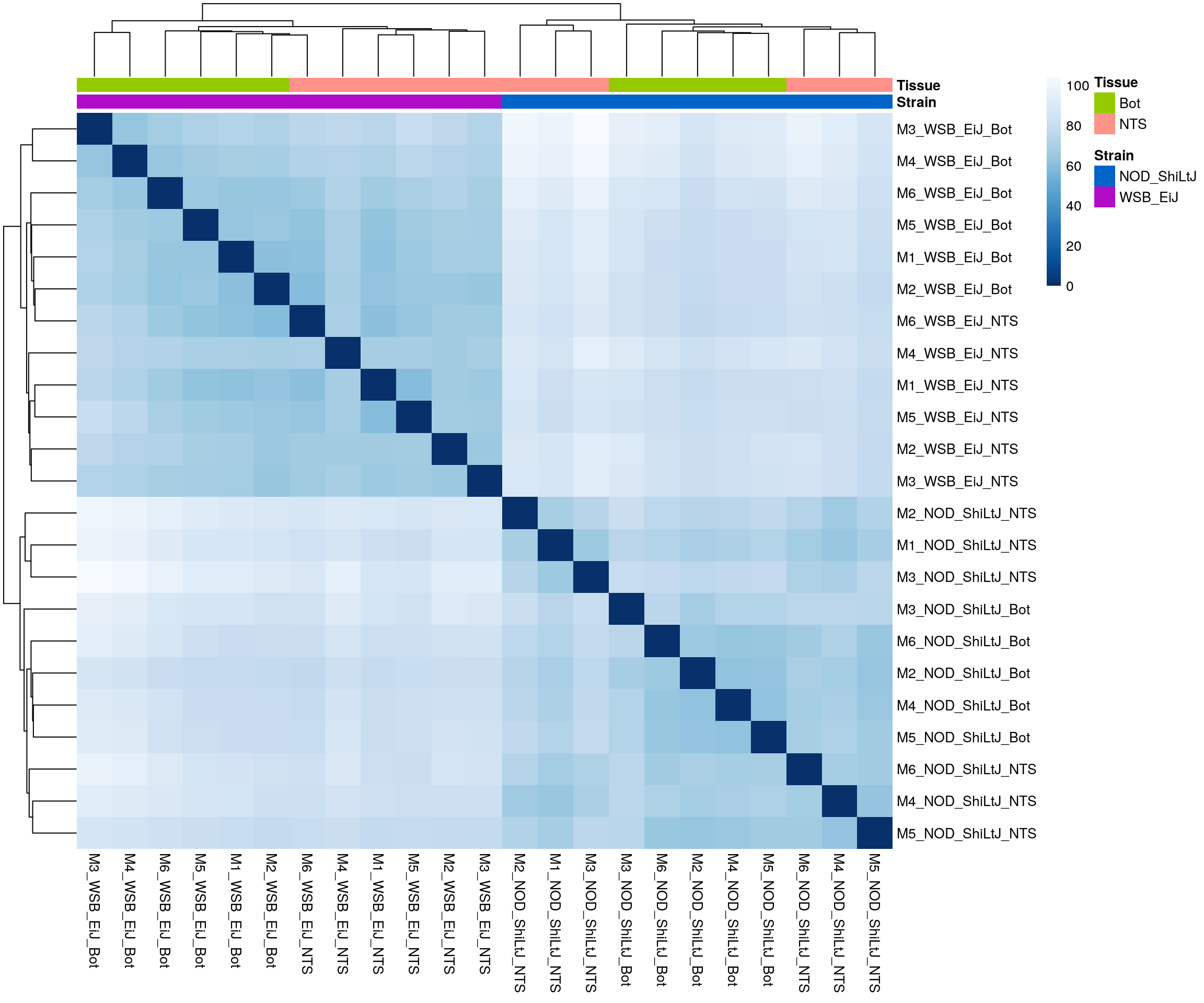
| Version | Author | Date |
|---|---|---|
| 414688f | xhyuo | 2021-08-09 |
#heatmap on correlation matrix
rld_cor <- cor(assay(rld))
pheatmap(rld_cor,
         annotation_col  = df,
         clustering_distance_rows = "correlation",
         clustering_distance_cols = "correlation",
         annotation_colors = list(Strain = c(NOD_ShiLtJ = "#0064C9",
                                             WSB_EiJ    ="#B10DC9"),
                                  Tissue = c(Bot = "#96ca00",
                                             NTS = "#ff9289")),
         border_color = NA)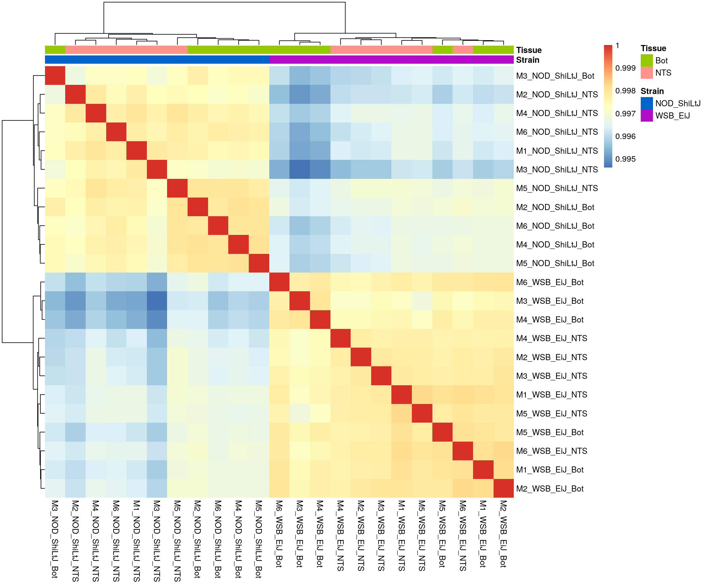
| Version | Author | Date |
|---|---|---|
| 414688f | xhyuo | 2021-08-09 |
#PCA plot
#Another way to visualize sample-to-sample distances is a principal components analysis (PCA).
pca.plot <- plotPCA(rld, intgroup = c("Strain", "Tissue"), returnData = FALSE)
pca.plot$data$name[!pca.plot$data$name %in% c("M6_WSB_EiJ_NTS", "M5_NOD_ShiLtJ_NTS")] = ""
pca.plot + geom_text(aes(label=name))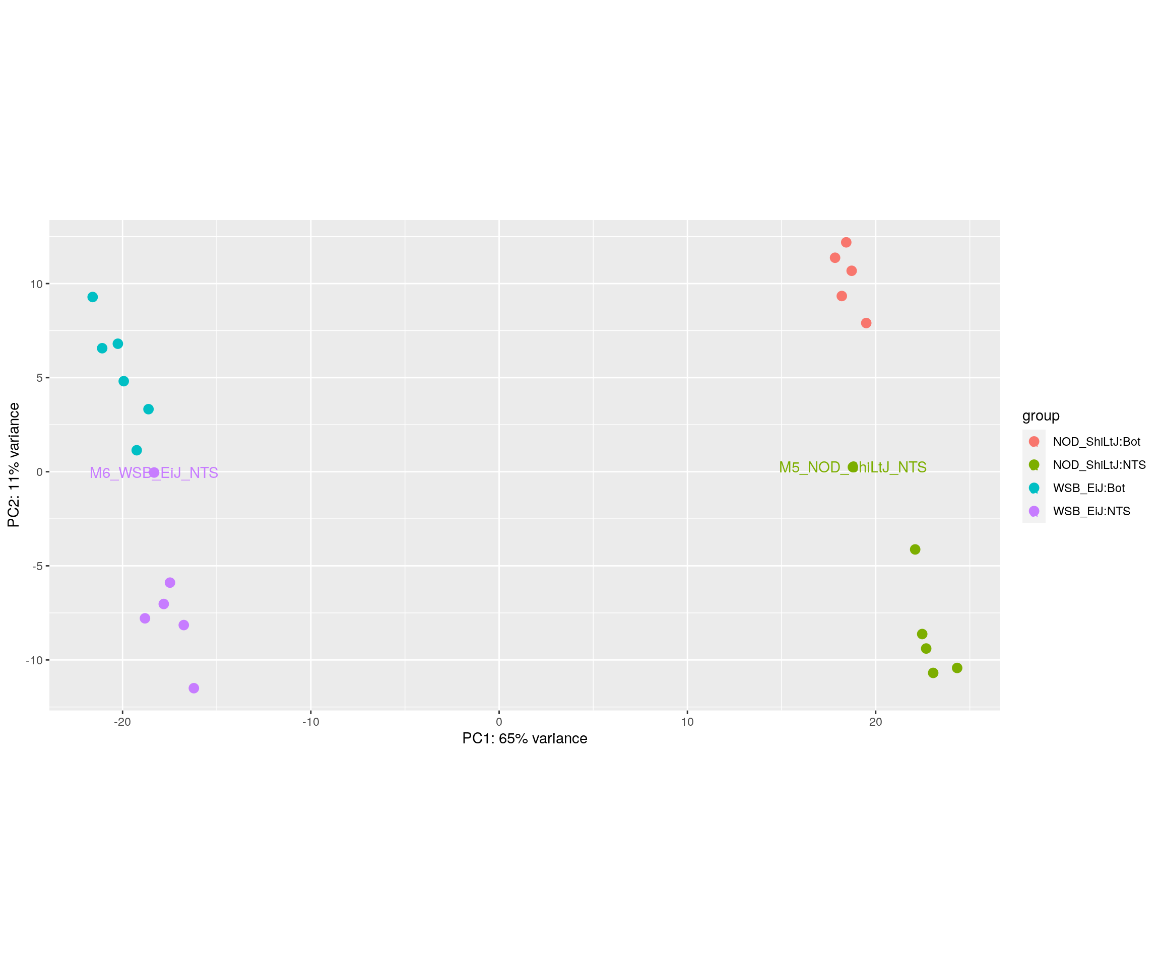
| Version | Author | Date |
|---|---|---|
| 414688f | xhyuo | 2021-08-09 |
Differential expression analysis with interaction term
design(ddsMat) <- ~Tissue + Strain + Tissue:Strain
#Running the differential expression pipeline
res <- DESeq(ddsMat)
estimating size factorsestimating dispersionsgene-wise dispersion estimatesmean-dispersion relationshipfinal dispersion estimatesfitting model and testingresultsNames(res)[1] "Intercept" "Tissue_NTS_vs_Bot"
[3] "Strain_WSB_EiJ_vs_NOD_ShiLtJ" "TissueNTS.StrainWSB_EiJ" The effect of Strain in Bot
#in Bot, WSB_EiJ compared with NOD_ShiLtJ
#Building the results table
res.tab.strain.in.Bot <- results(res, contrast=c("Strain","WSB_EiJ","NOD_ShiLtJ"), alpha = 0.05)
res.tab.strain.in.Bot
log2 fold change (MLE): Strain WSB_EiJ vs NOD_ShiLtJ
Wald test p-value: Strain WSB EiJ vs NOD ShiLtJ
DataFrame with 78620 rows and 6 columns
baseMean log2FoldChange lfcSE stat pvalue
<numeric> <numeric> <numeric> <numeric> <numeric>
ENSMUST00000192671 0.441721 -1.080778 4.367760 -0.247444 8.04564e-01
ENSMUST00000110582 531.841093 0.058942 0.100978 0.583711 5.59415e-01
ENSMUST00000110583 908.807431 0.508108 0.129210 3.932432 8.40907e-05
ENSMUST00000192674 2.222793 -1.510351 1.092876 -1.381996 1.66973e-01
ENSMUST00000110586 153.201898 0.164242 0.680124 0.241489 8.09176e-01
... ... ... ... ... ...
ENSMUST00000039949 13.31613 0.198163 0.549398 0.360692 0.7183299
ENSMUST00000098602 1.21233 -1.615111 3.751679 -0.430503 0.6668295
ENSMUST00000098603 1601.55262 0.333296 0.164288 2.028722 0.0424866
ENSMUST00000156039 71.49969 0.253834 0.310224 0.818229 0.4132265
ENSMUST00000022064 2.06784 -0.739195 2.543280 -0.290646 0.7713218
padj
<numeric>
ENSMUST00000192671 NA
ENSMUST00000110582 0.84298541
ENSMUST00000110583 0.00216242
ENSMUST00000192674 NA
ENSMUST00000110586 0.94664687
... ...
ENSMUST00000039949 0.914390
ENSMUST00000098602 NA
ENSMUST00000098603 0.221704
ENSMUST00000156039 0.752997
ENSMUST00000022064 NAsummary(res.tab.strain.in.Bot)
out of 78620 with nonzero total read count
adjusted p-value < 0.05
LFC > 0 (up)       : 2523, 3.2%
LFC < 0 (down)     : 3295, 4.2%
outliers [1]       : 469, 0.6%
low counts [2]     : 16430, 21%
(mean count < 3)
[1] see 'cooksCutoff' argument of ?results
[2] see 'independentFiltering' argument of ?results
table(res.tab.strain.in.Bot$padj < 0.05)
FALSE  TRUE
55903  5818
#We subset the results table to these genes and then sort it by the log2 fold change estimate to get the significant genes with the strongest down-regulation:
resSig.strain.in.Bot <- subset(res.tab.strain.in.Bot, padj < 0.05)
head(resSig.strain.in.Bot[order(resSig.strain.in.Bot$log2FoldChange), ])log2 fold change (MLE): Strain WSB_EiJ vs NOD_ShiLtJ
Wald test p-value: Strain WSB EiJ vs NOD ShiLtJ
DataFrame with 6 rows and 6 columns
baseMean log2FoldChange lfcSE stat pvalue
<numeric> <numeric> <numeric> <numeric> <numeric>
ENSMUST00000165515 4.98482 -21.7559 4.273955 -5.09035 3.57409e-07
ENSMUST00000134089 7.49242 -20.5268 2.633395 -7.79480 6.45091e-15
ENSMUST00000164868 4.52682 -20.4588 4.081304 -5.01280 5.36431e-07
ENSMUST00000065243 461.07625 -12.0506 0.862919 -13.96492 2.55202e-44
ENSMUST00000174728 361.13657 -11.9025 0.843932 -14.10358 3.60993e-45
ENSMUST00000065408 224.77361 -11.3820 0.867053 -13.12726 2.29810e-39
padj
<numeric>
ENSMUST00000165515 1.92829e-05
ENSMUST00000134089 1.07031e-12
ENSMUST00000164868 2.75450e-05
ENSMUST00000065243 1.96891e-41
ENSMUST00000174728 2.93169e-42
ENSMUST00000065408 1.49306e-36# with the strongest up-regulation:
head(resSig.strain.in.Bot[order(resSig.strain.in.Bot$log2FoldChange, decreasing = TRUE), ])log2 fold change (MLE): Strain WSB_EiJ vs NOD_ShiLtJ
Wald test p-value: Strain WSB EiJ vs NOD ShiLtJ
DataFrame with 6 rows and 6 columns
baseMean log2FoldChange lfcSE stat pvalue
<numeric> <numeric> <numeric> <numeric> <numeric>
ENSMUST00000028003 10.54097 21.2522 4.289327 4.95467 7.24541e-07
ENSMUST00000161573 11.31792 20.4717 2.849574 7.18412 6.76405e-13
ENSMUST00000112502 8.21463 19.1495 3.209191 5.96709 2.41523e-09
ENSMUST00000153532 7.87190 16.1163 3.687907 4.37005 1.24217e-05
ENSMUST00000084007 2183.04059 14.5223 0.927069 15.66474 2.63486e-55
ENSMUST00000111824 4140.20657 12.3019 0.489296 25.14196 1.73055e-139
padj
<numeric>
ENSMUST00000028003 3.59458e-05
ENSMUST00000161573 9.36062e-11
ENSMUST00000112502 2.06183e-07
ENSMUST00000153532 4.23975e-04
ENSMUST00000084007 2.85309e-52
ENSMUST00000111824 4.85505e-136#Visualization for res.tab.strain.in.Bot------
#Volcano plot
## Obtain logical vector regarding whether padj values are less than 0.05
threshold_OE <- (res.tab.strain.in.Bot$padj < 0.05 & !is.na(res.tab.strain.in.Bot$padj) & abs(res.tab.strain.in.Bot$log2FoldChange) >= 1)
## Determine the number of TRUE values
length(which(threshold_OE))[1] 2341## Add logical vector as a column (threshold) to the res.tab.strain.in.Bot
res.tab.strain.in.Bot$threshold <- threshold_OE
## Sort by ordered padj
res.tab.strain.in.Bot_ordered <- res.tab.strain.in.Bot %>%
data.frame() %>%
rownames_to_column(var="target_id") %>%
arrange(padj) %>%
mutate(genelabels = "") %>%
as_tibble() %>%
left_join(genes)Joining, by = "target_id"## Create a column to indicate which genes to label
res.tab.strain.in.Bot_ordered$genelabels[1:10] <- res.tab.strain.in.Bot_ordered$SYMBOL[1:10]
#display res.tab.strain.in.Bot_ordered
DT::datatable(res.tab.strain.in.Bot_ordered[res.tab.strain.in.Bot_ordered$threshold,],
filter = list(position = 'top', clear = FALSE),
options = list(pageLength = 40, scrollY = "300px", scrollX = "40px"),
caption = htmltools::tags$caption(style = 'caption-side: top; text-align: left; color:black; font-size:200% ;','DEG for WSB_EiJ vs NOD_ShiLtJ in Bot (fdr < 0.05)'))#Volcano plot
volcano.plot.strain.in.Bot <- ggplot(res.tab.strain.in.Bot_ordered) +
geom_point(aes(x = log2FoldChange, y = -log10(padj), colour = threshold)) +
scale_color_manual(values=c("blue", "red")) +
geom_text_repel(aes(x = log2FoldChange, y = -log10(padj),
label = genelabels,
size = 3.5)) +
ggtitle("DEG for WSB_EiJ vs NOD_ShiLtJ in Bot") +
xlab("log2 fold change") +
ylab("-log10 adjusted p-value") +
theme(legend.position = "none",
plot.title = element_text(size = rel(1.5), hjust = 0.5),
axis.title = element_text(size = rel(1.25)))
print(volcano.plot.strain.in.Bot)Warning: Removed 17026 rows containing missing values (geom_point).Warning: Removed 17026 rows containing missing values (geom_text_repel).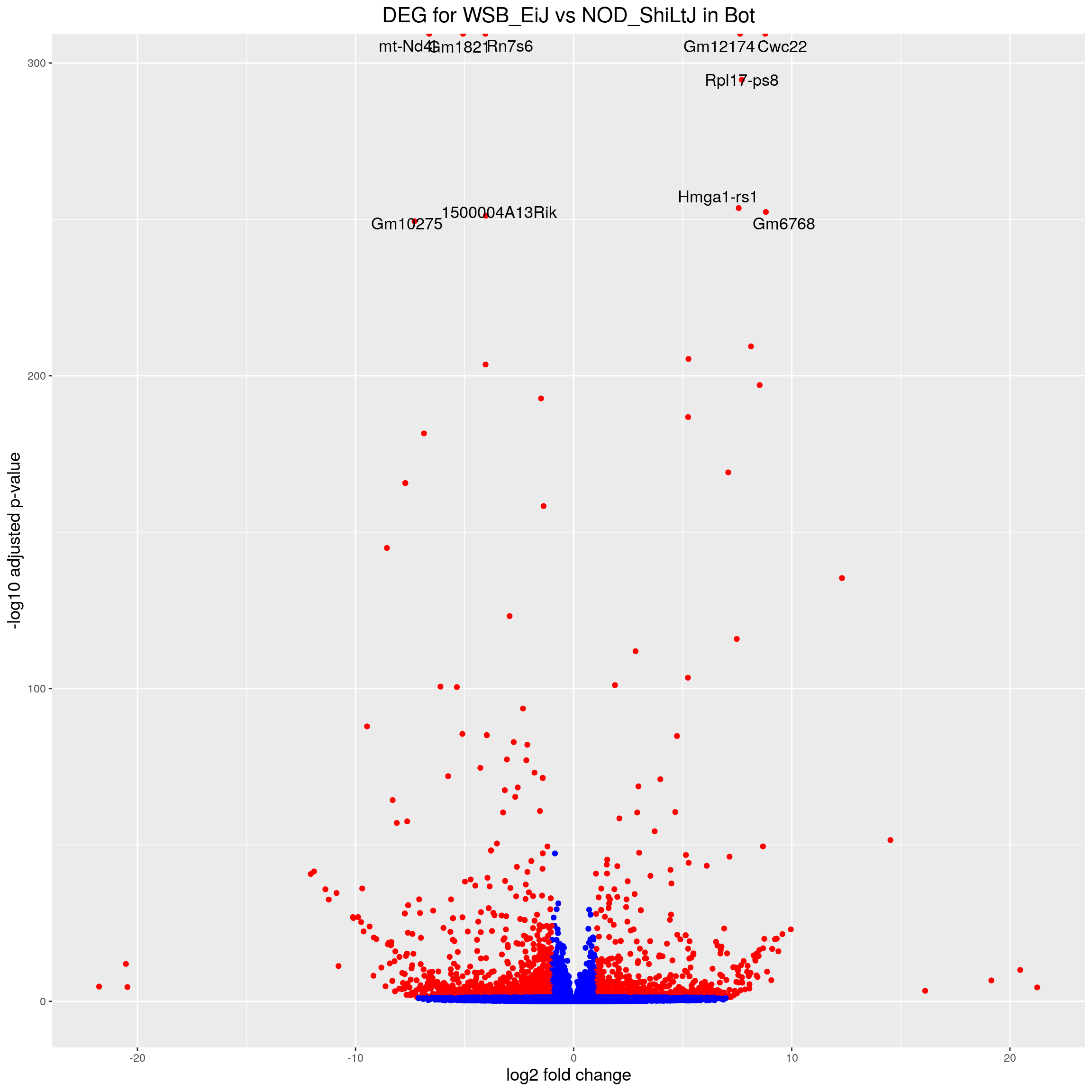
| Version | Author | Date |
|---|---|---|
| 414688f | xhyuo | 2021-08-09 |
#heatmap
# Extract normalized expression for significant genes fdr < 0.05 & abs(log2FoldChange) >= 1)
normalized_counts_sig.strain.in.Bot <- normalized_counts %>%
filter(gene %in% rownames(subset(resSig.strain.in.Bot, padj < 0.05 & abs(log2FoldChange) >= 1))) %>%
dplyr::select(-1) %>%
dplyr::select(contains("Bot"))
### Set a color palette
heat_colors <- brewer.pal(6, "YlOrRd")
#annotation
df <- as.data.frame(colData(ddsMat)[,c("Strain","Tissue")]) %>%
filter(Tissue == "Bot")
### Run pheatmap using the metadata data frame for the annotation
sig.strain.in.Bot.plot <- pheatmap(as.matrix(normalized_counts_sig.strain.in.Bot),
color = heat_colors,
cluster_rows = T,
show_rownames = F,
annotation_col = df,
annotation_colors = list(Strain = c(NOD_ShiLtJ = "#0064C9",
WSB_EiJ ="#B10DC9"),
Tissue = c(Bot = "#96ca00",
NTS = "#ff9289")),
border_color = NA,
fontsize = 10,
scale = "row",
fontsize_row = 10,
height = 20,
legend = FALSE,
annotation_legend = FALSE,
annotation_names_col = FALSE
#main = "Heatmap of the top DEGs in WSB_EiJ vs NOD_ShiLtJ
#in Bot (fdr < 0.05 & abs(log2FoldChange) >= 1)"
)
sig.strain.in.Bot.plot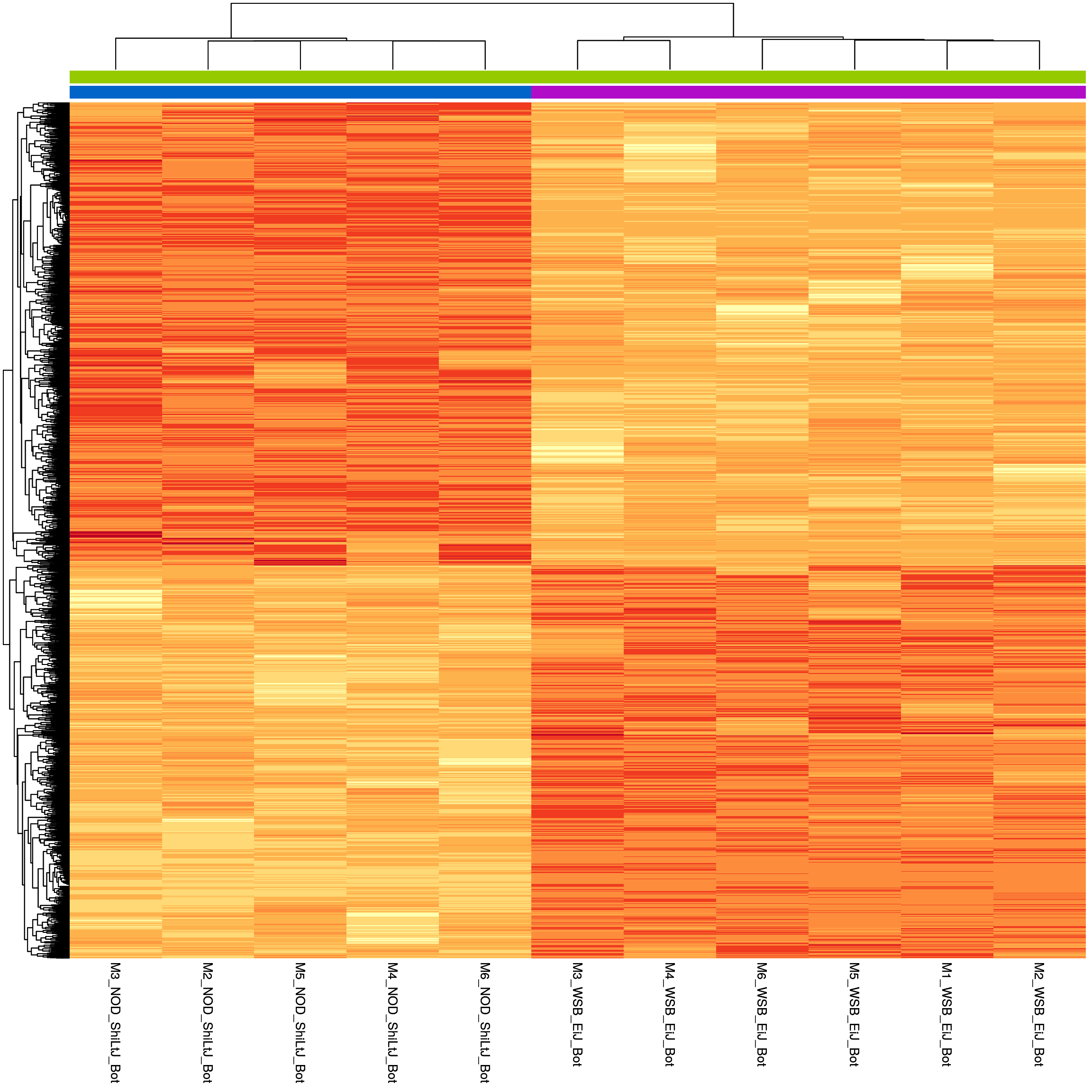
| Version | Author | Date |
|---|---|---|
| 414688f | xhyuo | 2021-08-09 |
#enrichment analysis for res.tab.strain.in.Bot-------
dbs <- c("WikiPathways_2019_Mouse",
"GO_Biological_Process_2021",
"GO_Cellular_Component_2021",
"GO_Molecular_Function_2021",
"KEGG_2019_Mouse",
"Mouse_Gene_Atlas",
"MGI_Mammalian_Phenotype_Level_4_2019")
#results (fdr < 0.05)------
resSig.strain.in.Bot.tab <- resSig.strain.in.Bot %>%
data.frame() %>%
rownames_to_column(var="target_id") %>%
as_tibble() %>%
left_join(genes)Joining, by = "target_id"#up-regulated genes WSB_EiJ vs NOD_ShiLtJ in Bot ---------------------------
up.genes <- resSig.strain.in.Bot.tab %>%
filter(log2FoldChange > 0) %>%
pull(SYMBOL)
#up-regulated genes enrichment
up.genes.enriched <- enrichr(as.character(na.omit(up.genes)), dbs)Uploading data to Enrichr... Done.
Querying WikiPathways_2019_Mouse... Done.
Querying GO_Biological_Process_2021... Done.
Querying GO_Cellular_Component_2021... Done.
Querying GO_Molecular_Function_2021... Done.
Querying KEGG_2019_Mouse... Done.
Querying Mouse_Gene_Atlas... Done.
Querying MGI_Mammalian_Phenotype_Level_4_2019... Done.
Parsing results... Done.for (j in 1:length(up.genes.enriched)){
up.genes.enriched[[j]] <- cbind(data.frame(Library = names(up.genes.enriched)[j]),up.genes.enriched[[j]])
}
up.genes.enriched <- do.call(rbind.data.frame, up.genes.enriched) %>%
filter(Adjusted.P.value <= 0.05) %>%
mutate(logpvalue = -log10(P.value)) %>%
arrange(desc(logpvalue))
#display up.genes.enriched
DT::datatable(up.genes.enriched,filter = list(position = 'top', clear = FALSE),
options = list(pageLength = 40, scrollY = "300px", scrollX = "40px"))#barpot
up.genes.enriched.plot.in.Bot <- up.genes.enriched %>%
filter(Adjusted.P.value <= 0.01) %>%
mutate(Term = fct_reorder(Term, -logpvalue)) %>%
ggplot(data = ., aes(x = Term, y = logpvalue, fill = Library, label = Overlap)) +
geom_bar(stat = "identity") +
geom_text(position = position_dodge(width = 0.9),
hjust = 0) +
theme_bw() +
ylab("-log(p.value)") +
xlab("") +
ggtitle("Enrichment of up-regulated genes for WSB_EiJ vs NOD_ShiLtJ \nin Bot (Adjusted.P.value <= 0.01)") +
theme(plot.background = element_blank() ,
panel.border = element_blank(),
panel.background = element_blank(),
#legend.position = "none",
plot.title = element_text(hjust = 0),
panel.grid.major = element_blank(),
panel.grid.minor = element_blank()) +
theme(axis.line = element_line(color = 'black')) +
theme(axis.title.x = element_text(size = 12, vjust=-0.5)) +
theme(axis.title.y = element_text(size = 12, vjust= 1.0)) +
theme(axis.text = element_text(size = 12)) +
theme(plot.title = element_text(size = 12)) +
coord_flip()
up.genes.enriched.plot.in.Bot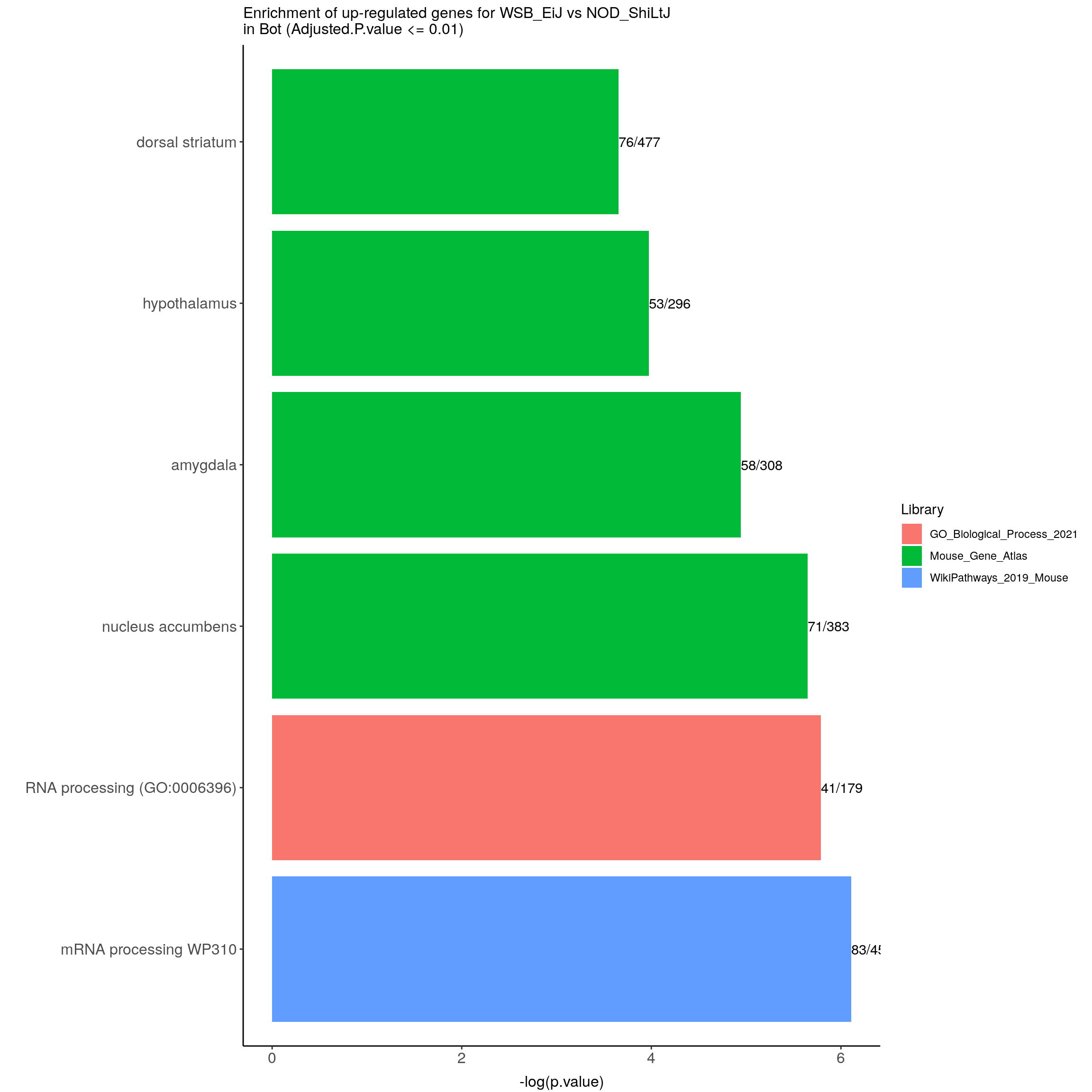
| Version | Author | Date |
|---|---|---|
| 414688f | xhyuo | 2021-08-09 |
#down-regulated genes WSB_EiJ vs NOD_ShiLtJ in Bot---------------------------
down.genes <- resSig.strain.in.Bot.tab %>%
filter(log2FoldChange < 0) %>%
pull(SYMBOL)
#down-regulated genes enrichment
down.genes.enriched <- enrichr(as.character(na.omit(down.genes)), dbs)Uploading data to Enrichr... Done.
Querying WikiPathways_2019_Mouse... Done.
Querying GO_Biological_Process_2021... Done.
Querying GO_Cellular_Component_2021... Done.
Querying GO_Molecular_Function_2021... Done.
Querying KEGG_2019_Mouse... Done.
Querying Mouse_Gene_Atlas... Done.
Querying MGI_Mammalian_Phenotype_Level_4_2019... Done.
Parsing results... Done.for (j in 1:length(down.genes.enriched)){
down.genes.enriched[[j]] <- cbind(data.frame(Library = names(down.genes.enriched)[j]),down.genes.enriched[[j]])
}
down.genes.enriched <- do.call(rbind.data.frame, down.genes.enriched) %>%
filter(Adjusted.P.value <= 0.05) %>%
mutate(logpvalue = -log10(P.value)) %>%
arrange(desc(logpvalue))
#display down.genes.enriched
DT::datatable(down.genes.enriched,filter = list(position = 'top', clear = FALSE),
options = list(pageLength = 40, scrollY = "300px", scrollX = "40px"))#barpot
down.genes.enriched.plot.in.Bot <- down.genes.enriched %>%
filter(Adjusted.P.value <= 0.001) %>%
mutate(Term = fct_reorder(Term, -logpvalue)) %>%
ggplot(data = ., aes(x = Term, y = logpvalue, fill = Library, label = Overlap)) +
geom_bar(stat = "identity") +
geom_text(position = position_dodge(width = 0.9),
hjust = 0) +
theme_bw() +
ylab("-log(p.value)") +
xlab("") +
ggtitle("Enrichment of down-regulated genes for WSB_EiJ vs NOD_ShiLtJ \nin Bot (Adjusted.P.value <= 0.001)") +
theme(plot.background = element_blank() ,
panel.border = element_blank(),
panel.background = element_blank(),
#legend.position = "none",
plot.title = element_text(hjust = 0),
panel.grid.major = element_blank(),
panel.grid.minor = element_blank()) +
theme(axis.line = element_line(color = 'black')) +
theme(axis.title.x = element_text(size = 12, vjust=-0.5)) +
theme(axis.title.y = element_text(size = 12, vjust= 1.0)) +
theme(axis.text = element_text(size = 12)) +
theme(plot.title = element_text(size = 12)) +
coord_flip()
down.genes.enriched.plot.in.Bot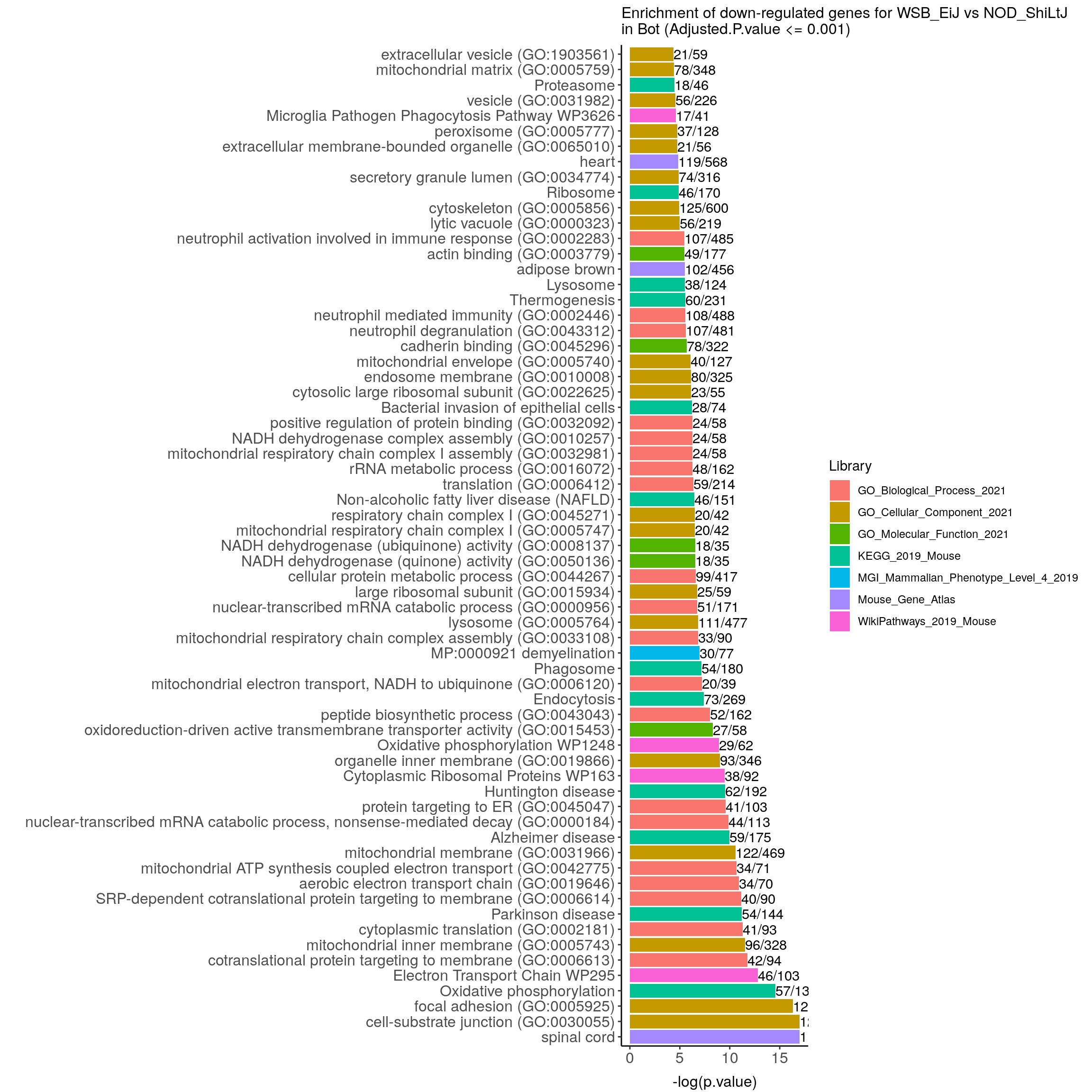
| Version | Author | Date |
|---|---|---|
| 414688f | xhyuo | 2021-08-09 |
The effect of Strain in NTS
#This is, by definition, the main effect plus the interaction term
#Building the results table
res.tab.strain.in.NTS <- results(res, list(c("Strain_WSB_EiJ_vs_NOD_ShiLtJ",
"TissueNTS.StrainWSB_EiJ")), alpha = 0.05)
summary(res.tab.strain.in.NTS)
out of 78620 with nonzero total read count
adjusted p-value < 0.05
LFC > 0 (up) : 2011, 2.6%
LFC < 0 (down) : 2792, 3.6%
outliers [1] : 469, 0.6%
low counts [2] : 14944, 19%
(mean count < 3)
[1] see 'cooksCutoff' argument of ?results
[2] see 'independentFiltering' argument of ?resultstable(res.tab.strain.in.NTS$padj < 0.05)
FALSE TRUE
58404 4803 #We subset the results table to these genes and then sort it by the log2 fold change estimate to get the significant genes with the strongest down-regulation:
resSig.strain.in.NTS <- subset(res.tab.strain.in.NTS, padj < 0.05)
head(resSig.strain.in.NTS[order(resSig.strain.in.NTS$log2FoldChange), ])log2 fold change (MLE): Strain_WSB_EiJ_vs_NOD_ShiLtJ+TissueNTS.StrainWSB_EiJ effect
Wald test p-value: Strain_WSB_EiJ_vs_NOD_ShiLtJ+TissueNTS.StrainWSB_EiJ effect
DataFrame with 6 rows and 6 columns
baseMean log2FoldChange lfcSE stat pvalue
<numeric> <numeric> <numeric> <numeric> <numeric>
ENSMUST00000165515 4.98482 -26.4960 4.090742 -6.47707 9.35188e-11
ENSMUST00000174728 361.13657 -12.1041 0.842891 -14.36024 9.19055e-47
ENSMUST00000065243 461.07625 -11.7374 0.860276 -13.64372 2.20035e-42
ENSMUST00000198699 237.43543 -11.5486 0.890410 -12.96995 1.81150e-38
ENSMUST00000065408 224.77361 -11.2900 0.864021 -13.06686 5.09226e-39
ENSMUST00000140065 172.96767 -10.5396 0.840776 -12.53559 4.76826e-36
padj
<numeric>
ENSMUST00000165515 9.54934e-09
ENSMUST00000174728 7.26134e-44
ENSMUST00000065243 1.54531e-39
ENSMUST00000198699 1.12255e-35
ENSMUST00000065408 3.21867e-36
ENSMUST00000140065 2.71520e-33# with the strongest up-regulation:
head(resSig.strain.in.NTS[order(resSig.strain.in.NTS$log2FoldChange, decreasing = TRUE), ])log2 fold change (MLE): Strain_WSB_EiJ_vs_NOD_ShiLtJ+TissueNTS.StrainWSB_EiJ effect
Wald test p-value: Strain_WSB_EiJ_vs_NOD_ShiLtJ+TissueNTS.StrainWSB_EiJ effect
DataFrame with 6 rows and 6 columns
baseMean log2FoldChange lfcSE stat pvalue
<numeric> <numeric> <numeric> <numeric> <numeric>
ENSMUST00000028003 10.5410 24.1998 4.082988 5.92697 3.08570e-09
ENSMUST00000123819 33.9746 22.6318 1.722338 13.14014 1.93872e-39
ENSMUST00000111646 30.6297 20.7893 2.343371 8.87155 7.21357e-19
ENSMUST00000111824 4140.2066 15.3016 0.837386 18.27307 1.35613e-74
ENSMUST00000084007 2183.0406 13.0943 0.825261 15.86689 1.07440e-56
ENSMUST00000077016 134.9254 10.5674 0.876532 12.05596 1.80415e-33
padj
<numeric>
ENSMUST00000028003 2.41085e-07
ENSMUST00000123819 1.25041e-36
ENSMUST00000111646 1.50976e-16
ENSMUST00000111824 1.86341e-71
ENSMUST00000084007 1.11328e-53
ENSMUST00000077016 9.34712e-31#Visualization for res.tab.strain.in.NTS------
#Volcano plot
## Obtain logical vector regarding whether padj values are less than 0.05
threshold_OE <- (res.tab.strain.in.NTS$padj < 0.05 & !is.na(res.tab.strain.in.NTS$padj) & abs(res.tab.strain.in.NTS$log2FoldChange) >= 1)
## Determine the number of TRUE values
length(which(threshold_OE))[1] 2281## Add logical vector as a column (threshold) to the res.tab.strain.in.NTS
res.tab.strain.in.NTS$threshold <- threshold_OE
## Sort by ordered padj
res.tab.strain.in.NTS_ordered <- res.tab.strain.in.NTS %>%
data.frame() %>%
rownames_to_column(var="target_id") %>%
arrange(padj) %>%
mutate(genelabels = "") %>%
as_tibble() %>%
left_join(genes)Joining, by = "target_id"## Create a column to indicate which genes to label
res.tab.strain.in.NTS_ordered$genelabels[1:10] <- res.tab.strain.in.NTS_ordered$SYMBOL[1:10]
#display res.tab.strain.in.NTS_ordered
DT::datatable(res.tab.strain.in.NTS_ordered[res.tab.strain.in.NTS_ordered$threshold,],
filter = list(position = 'top', clear = FALSE),
options = list(pageLength = 40, scrollY = "300px", scrollX = "40px"),
caption = htmltools::tags$caption(style = 'caption-side: top; text-align: left; color:black; font-size:200% ;','DEG for WSB_EiJ vs NOD_ShiLtJ in NTS (fdr < 0.05)'))#Volcano plot
volcano.plot.strain.in.NTS <- ggplot(res.tab.strain.in.NTS_ordered) +
geom_point(aes(x = log2FoldChange, y = -log10(padj), colour = threshold)) +
scale_color_manual(values=c("blue", "red")) +
geom_text_repel(aes(x = log2FoldChange, y = -log10(padj),
label = genelabels,
size = 3.5)) +
ggtitle("DEG for WSB_EiJ vs NOD_ShiLtJ in NTS") +
xlab("log2 fold change") +
ylab("-log10 adjusted p-value") +
theme(legend.position = "none",
plot.title = element_text(size = rel(1.5), hjust = 0.5),
axis.title = element_text(size = rel(1.25)))
print(volcano.plot.strain.in.NTS)Warning: Removed 15531 rows containing missing values (geom_point).Warning: Removed 15531 rows containing missing values (geom_text_repel).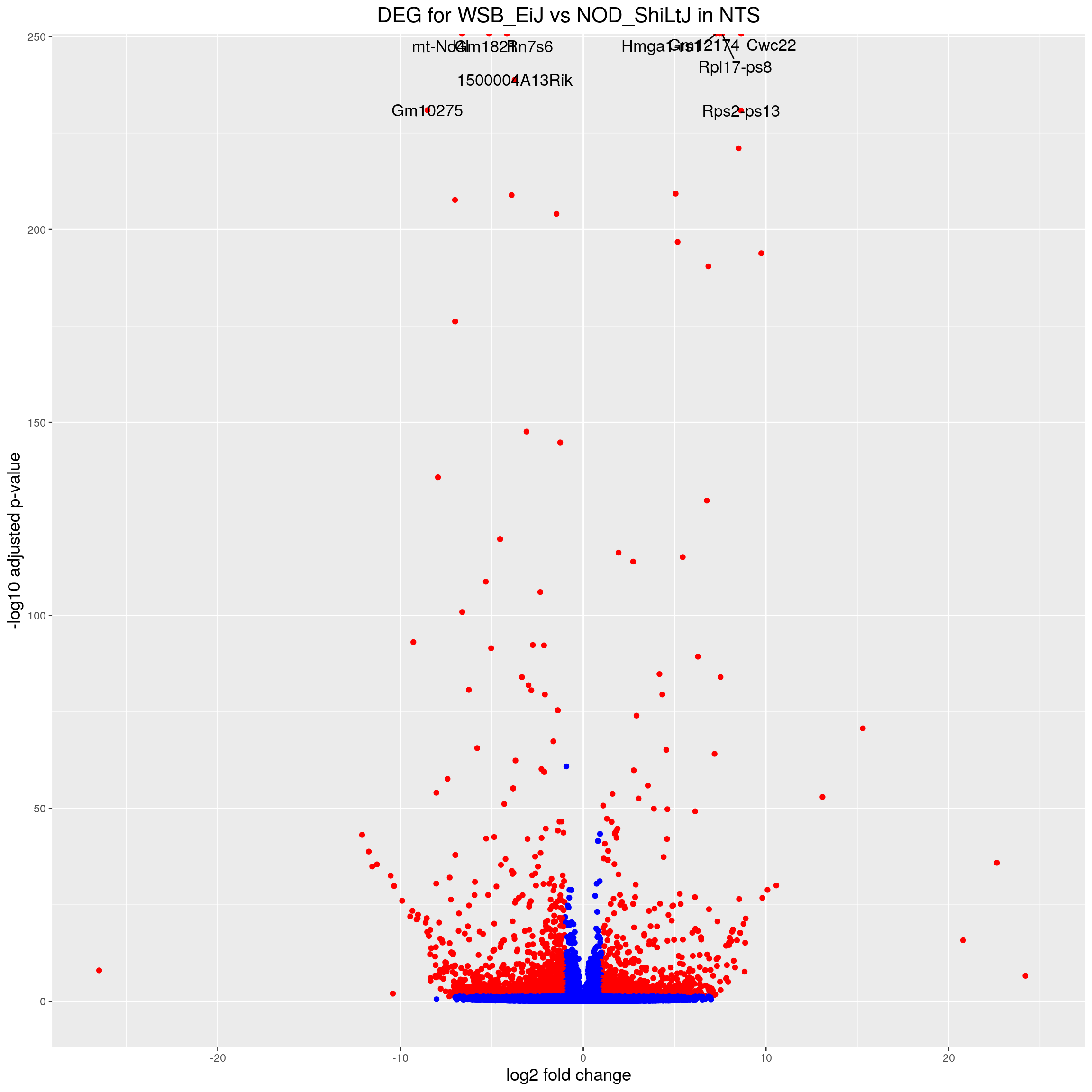
| Version | Author | Date |
|---|---|---|
| 414688f | xhyuo | 2021-08-09 |
#heatmap
# Extract normalized expression for significant genes fdr < 0.05 & abs(log2FoldChange) >= 1)
normalized_counts_sig.strain.in.NTS <- normalized_counts %>%
filter(gene %in% rownames(subset(resSig.strain.in.NTS, padj < 0.05 & abs(log2FoldChange) >= 1))) %>%
dplyr::select(-1) %>%
dplyr::select(contains("NTS"))
### Set a color palette
heat_colors <- brewer.pal(6, "YlOrRd")
#annotation
df <- as.data.frame(colData(ddsMat)[,c("Strain","Tissue")]) %>%
filter(Tissue == "NTS")
### Run pheatmap using the metadata data frame for the annotation
sig.strain.in.NTS.plot <- pheatmap(as.matrix(normalized_counts_sig.strain.in.NTS),
color = heat_colors,
cluster_rows = T,
show_rownames = F,
annotation_col = df,
annotation_colors = list(Strain = c(NOD_ShiLtJ = "#0064C9",
WSB_EiJ ="#B10DC9"),
Tissue = c(Bot = "#96ca00",
NTS = "#ff9289")),
border_color = NA,
fontsize = 10,
scale = "row",
fontsize_row = 10,
height = 20, #legend = FALSE, annotation_legend = FALSE, annotation_names_col = FALSE,
#main = "Heatmap of the top DEGs in WSB_EiJ vs NOD_ShiLtJ in NTS (fdr < 0.05 & abs(log2FoldChange) >= 1)"
)
sig.strain.in.NTS.plot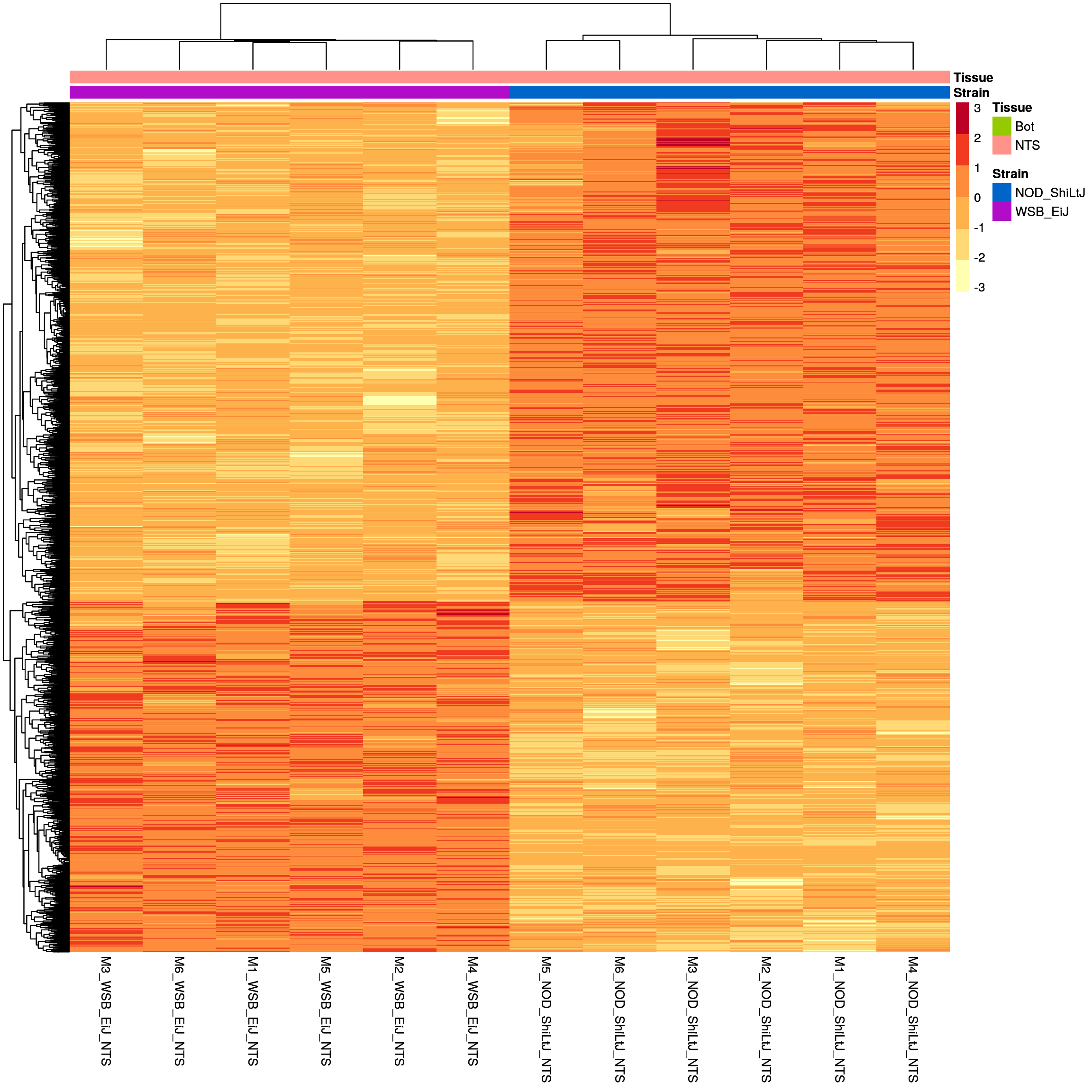
| Version | Author | Date |
|---|---|---|
| 414688f | xhyuo | 2021-08-09 |
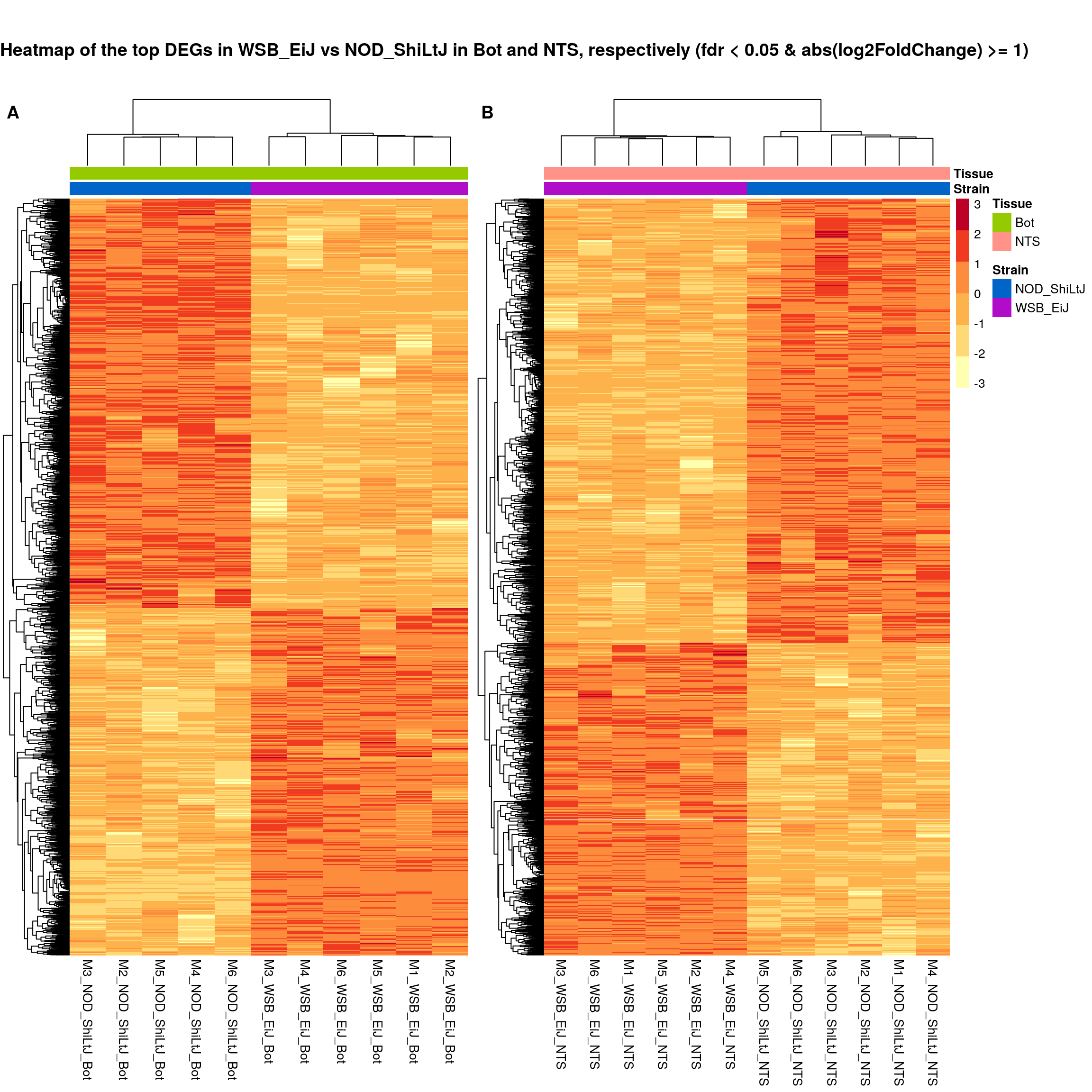
#plot sig.strain.in.Bot.plot and sig.strain.in.NTS.plot together-------
ht.map2.plot = plot_grid(as.grob(sig.strain.in.Bot.plot),
as.grob(sig.strain.in.NTS.plot),
align = "h", rel_widths = c(1, 1.3),
labels = c('A', 'B'))
#add title
# now add the title
title <- ggdraw() +
draw_label(
"Heatmap of the top DEGs in WSB_EiJ vs NOD_ShiLtJ in Bot and NTS, respectively (fdr < 0.05 & abs(log2FoldChange) >= 1)",
fontface = 'bold',
x = 0,
hjust = 0
)
plot_grid(
title,
ht.map2.plot,
ncol = 1,
# rel_heights values control vertical title margins
rel_heights = c(0.1, 1)
)
| Version | Author | Date |
|---|---|---|
| 414688f | xhyuo | 2021-08-09 |
#logFC heatmap on both Bot and NTS top DEGs-----
restop.tab.in.Bot.NTS <- full_join(res.tab.strain.in.Bot_ordered,
res.tab.strain.in.NTS_ordered,
by = c("ENSEMBL", "SYMBOL")) %>%
filter((ENSEMBL %in% res.tab.strain.in.Bot_ordered$ENSEMBL[1:30]) | (ENSEMBL %in% res.tab.strain.in.NTS_ordered$ENSEMBL[1:30]))
restop.tab.in.Bot.NTS.mat <- as.matrix(restop.tab.in.Bot.NTS[, c("log2FoldChange.x", "log2FoldChange.y")])
rownames(restop.tab.in.Bot.NTS.mat) <-
ifelse(is.na(restop.tab.in.Bot.NTS$SYMBOL),
restop.tab.in.Bot.NTS$ENSEMBL,
paste0(restop.tab.in.Bot.NTS$SYMBOL,":", restop.tab.in.Bot.NTS$ENSEMBL))
colnames(restop.tab.in.Bot.NTS.mat) <- c("Bot", "NTS")
#heatmap
### Run pheatmap using the metadata data frame for the annotation
pheatmap(restop.tab.in.Bot.NTS.mat,
color = colorpanel(1000, "blue", "white", "red"),
cluster_rows = T,
show_rownames = T,
border_color = NA,
fontsize = 10,
fontsize_row = 8,
height = 25,
main = "Heatmap of log2FoldChange for the top 30 DEGs in Bot and NTS")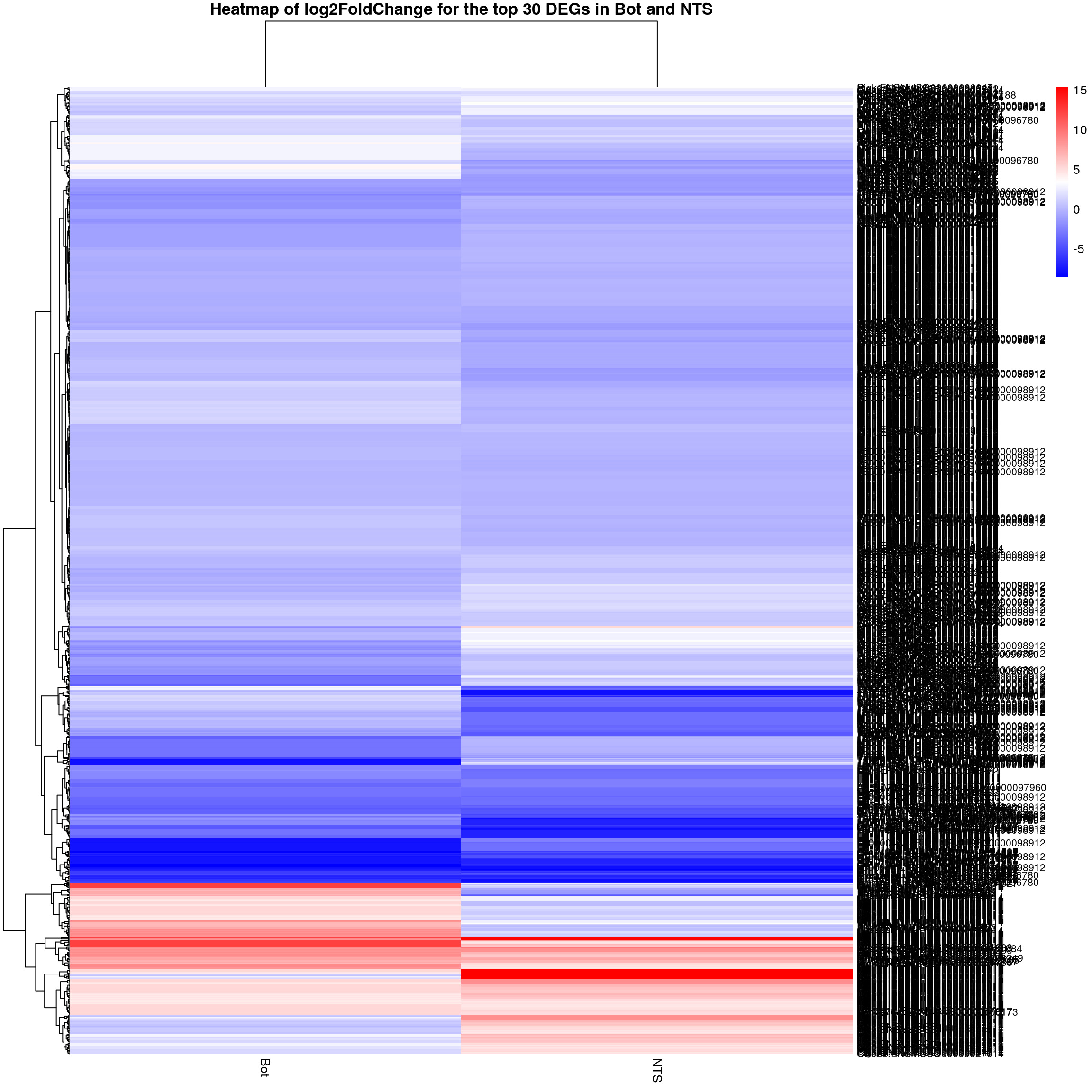
| Version | Author | Date |
|---|---|---|
| 414688f | xhyuo | 2021-08-09 |
#enrichment analysis for res.tab.strain.in.NTS-------
dbs <- c("WikiPathways_2019_Mouse",
"GO_Biological_Process_2021",
"GO_Cellular_Component_2021",
"GO_Molecular_Function_2021",
"KEGG_2019_Mouse",
"Mouse_Gene_Atlas",
"MGI_Mammalian_Phenotype_Level_4_2019")
#results (fdr < 0.05)------
resSig.strain.in.NTS.tab <- resSig.strain.in.NTS %>%
data.frame() %>%
rownames_to_column(var="target_id") %>%
as_tibble() %>%
left_join(genes)Joining, by = "target_id"#up-regulated genes WSB_EiJ vs NOD_ShiLtJ in NTS ---------------------------
up.genes <- resSig.strain.in.NTS.tab %>%
filter(log2FoldChange > 0) %>%
pull(SYMBOL)
#up-regulated genes enrichment
up.genes.enriched <- enrichr(as.character(na.omit(up.genes)), dbs)Uploading data to Enrichr... Done.
Querying WikiPathways_2019_Mouse... Done.
Querying GO_Biological_Process_2021... Done.
Querying GO_Cellular_Component_2021... Done.
Querying GO_Molecular_Function_2021... Done.
Querying KEGG_2019_Mouse... Done.
Querying Mouse_Gene_Atlas... Done.
Querying MGI_Mammalian_Phenotype_Level_4_2019... Done.
Parsing results... Done.for (j in 1:length(up.genes.enriched)){
up.genes.enriched[[j]] <- cbind(data.frame(Library = names(up.genes.enriched)[j]),up.genes.enriched[[j]])
}
up.genes.enriched <- do.call(rbind.data.frame, up.genes.enriched) %>%
filter(Adjusted.P.value <= 0.2) %>%
mutate(logpvalue = -log10(P.value)) %>%
arrange(desc(logpvalue))
#display up.genes.enriched
DT::datatable(up.genes.enriched,filter = list(position = 'top', clear = FALSE),
options = list(pageLength = 40, scrollY = "300px", scrollX = "40px"))#barpot
up.genes.enriched.plot.in.NTS <- up.genes.enriched %>%
filter(Adjusted.P.value <= 0.2) %>%
mutate(Term = fct_reorder(Term, -logpvalue)) %>%
ggplot(data = ., aes(x = Term, y = logpvalue, fill = Library, label = Overlap)) +
geom_bar(stat = "identity") +
geom_text(position = position_dodge(width = 0.9),
hjust = 0) +
theme_bw() +
ylab("-log(p.value)") +
xlab("") +
ggtitle("Enrichment of up-regulated genes for WSB_EiJ vs NOD_ShiLtJ \nin NTS (Adjusted.P.value <= 0.2)") +
theme(plot.background = element_blank() ,
panel.border = element_blank(),
panel.background = element_blank(),
#legend.position = "none",
plot.title = element_text(hjust = 0),
panel.grid.major = element_blank(),
panel.grid.minor = element_blank()) +
theme(axis.line = element_line(color = 'black')) +
theme(axis.title.x = element_text(size = 12, vjust=-0.5)) +
theme(axis.title.y = element_text(size = 12, vjust= 1.0)) +
theme(axis.text = element_text(size = 12)) +
theme(plot.title = element_text(size = 12)) +
coord_flip()
up.genes.enriched.plot.in.NTS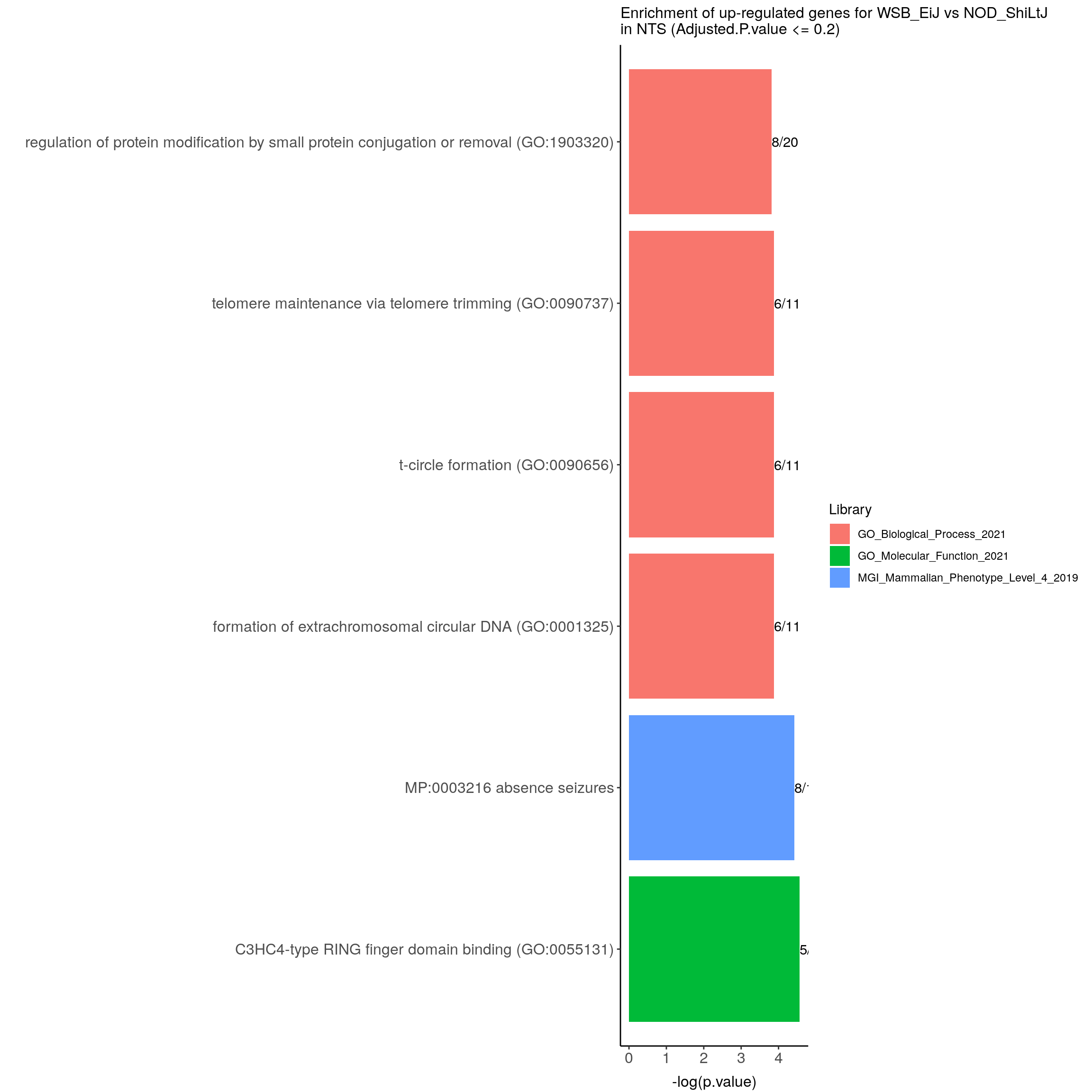
| Version | Author | Date |
|---|---|---|
| 414688f | xhyuo | 2021-08-09 |
#down-regulated genes WSB_EiJ vs NOD_ShiLtJ in NTS---------------------------
down.genes <- resSig.strain.in.NTS.tab %>%
filter(log2FoldChange < 0) %>%
pull(SYMBOL)
#down-regulated genes enrichment
down.genes.enriched <- enrichr(as.character(na.omit(down.genes)), dbs)Uploading data to Enrichr... Done.
Querying WikiPathways_2019_Mouse... Done.
Querying GO_Biological_Process_2021... Done.
Querying GO_Cellular_Component_2021... Done.
Querying GO_Molecular_Function_2021... Done.
Querying KEGG_2019_Mouse... Done.
Querying Mouse_Gene_Atlas... Done.
Querying MGI_Mammalian_Phenotype_Level_4_2019... Done.
Parsing results... Done.for (j in 1:length(down.genes.enriched)){
down.genes.enriched[[j]] <- cbind(data.frame(Library = names(down.genes.enriched)[j]),down.genes.enriched[[j]])
}
down.genes.enriched <- do.call(rbind.data.frame, down.genes.enriched) %>%
filter(Adjusted.P.value <= 0.05) %>%
mutate(logpvalue = -log10(P.value)) %>%
arrange(desc(logpvalue))
#display down.genes.enriched
DT::datatable(down.genes.enriched,filter = list(position = 'top', clear = FALSE),
options = list(pageLength = 40, scrollY = "300px", scrollX = "40px"))#barpot
down.genes.enriched.plot.in.NTS <- down.genes.enriched %>%
filter(Adjusted.P.value <= 0.001) %>%
mutate(Term = fct_reorder(Term, -logpvalue)) %>%
ggplot(data = ., aes(x = Term, y = logpvalue, fill = Library, label = Overlap)) +
geom_bar(stat = "identity") +
geom_text(position = position_dodge(width = 0.9),
hjust = 0) +
theme_bw() +
ylab("-log(p.value)") +
xlab("") +
ggtitle("Enrichment of down-regulated genes for WSB_EiJ vs NOD_ShiLtJ \nin NTS (Adjusted.P.value <= 0.001)") +
theme(plot.background = element_blank() ,
panel.border = element_blank(),
panel.background = element_blank(),
#legend.position = "none",
plot.title = element_text(hjust = 0),
panel.grid.major = element_blank(),
panel.grid.minor = element_blank()) +
theme(axis.line = element_line(color = 'black')) +
theme(axis.title.x = element_text(size = 12, vjust=-0.5)) +
theme(axis.title.y = element_text(size = 12, vjust= 1.0)) +
theme(axis.text = element_text(size = 12)) +
theme(plot.title = element_text(size = 12)) +
coord_flip()
down.genes.enriched.plot.in.NTS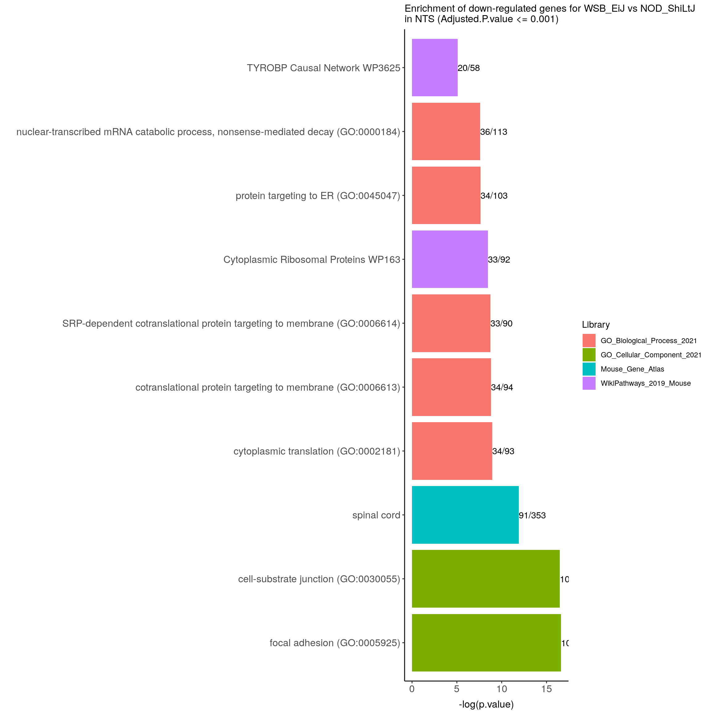
| Version | Author | Date |
|---|---|---|
| 414688f | xhyuo | 2021-08-09 |
Differential expression analysis with interaction term and one outlier removed
design(ddsMat) <- ~Tissue + Strain + Tissue:Strain
ddsMat <- ddsMat[,-which(colnames(ddsMat) == "M6_WSB_EiJ_NTS")] # remove outlier
#Running the differential expression pipeline
res <- DESeq(ddsMat)estimating size factorsestimating dispersionsgene-wise dispersion estimatesmean-dispersion relationshipfinal dispersion estimatesfitting model and testingresultsNames(res)[1] "Intercept" "Tissue_NTS_vs_Bot"
[3] "Strain_WSB_EiJ_vs_NOD_ShiLtJ" "TissueNTS.StrainWSB_EiJ" The effect of Strain in Bot with one outlier removed
#in Bot, WSB_EiJ compared with NOD_ShiLtJ
#Building the results table
res.tab.strain.in.Bot <- results(res, contrast=c("Strain","WSB_EiJ","NOD_ShiLtJ"), alpha = 0.05)
res.tab.strain.in.Botlog2 fold change (MLE): Strain WSB_EiJ vs NOD_ShiLtJ
Wald test p-value: Strain WSB EiJ vs NOD ShiLtJ
DataFrame with 78620 rows and 6 columns
baseMean log2FoldChange lfcSE stat pvalue
<numeric> <numeric> <numeric> <numeric> <numeric>
ENSMUST00000192671 0.459346 -1.0804316 4.279522 -0.252466 0.800681271
ENSMUST00000110582 530.746695 0.0592792 0.103421 0.573184 0.566520324
ENSMUST00000110583 907.010297 0.5084294 0.132319 3.842458 0.000121808
ENSMUST00000192674 2.113705 -1.5141230 1.150359 -1.316218 0.188100860
ENSMUST00000110586 151.330222 0.1648888 0.694086 0.237563 0.812220400
... ... ... ... ... ...
ENSMUST00000039949 13.09378 0.198402 0.566288 0.350355 0.7260721
ENSMUST00000098602 1.26018 -1.615787 3.679433 -0.439140 0.6605599
ENSMUST00000098603 1550.64239 0.333582 0.137660 2.423225 0.0153834
ENSMUST00000156039 70.62355 0.254057 0.318210 0.798395 0.4246412
ENSMUST00000022064 2.14923 -0.740364 2.449696 -0.302227 0.7624792
padj
<numeric>
ENSMUST00000192671 NA
ENSMUST00000110582 0.84836412
ENSMUST00000110583 0.00295977
ENSMUST00000192674 NA
ENSMUST00000110586 0.94802751
... ...
ENSMUST00000039949 0.918171
ENSMUST00000098602 NA
ENSMUST00000098603 0.114173
ENSMUST00000156039 0.763123
ENSMUST00000022064 NAsummary(res.tab.strain.in.Bot)
out of 78609 with nonzero total read count
adjusted p-value < 0.05
LFC > 0 (up) : 2471, 3.1%
LFC < 0 (down) : 3270, 4.2%
outliers [1] : 477, 0.61%
low counts [2] : 16438, 21%
(mean count < 3)
[1] see 'cooksCutoff' argument of ?results
[2] see 'independentFiltering' argument of ?resultstable(res.tab.strain.in.Bot$padj < 0.05)
FALSE TRUE
55953 5741 #We subset the results table to these genes and then sort it by the log2 fold change estimate to get the significant genes with the strongest down-regulation:
resSig.strain.in.Bot <- subset(res.tab.strain.in.Bot, padj < 0.05)
head(resSig.strain.in.Bot[order(resSig.strain.in.Bot$log2FoldChange), ])log2 fold change (MLE): Strain WSB_EiJ vs NOD_ShiLtJ
Wald test p-value: Strain WSB EiJ vs NOD ShiLtJ
DataFrame with 6 rows and 6 columns
baseMean log2FoldChange lfcSE stat pvalue
<numeric> <numeric> <numeric> <numeric> <numeric>
ENSMUST00000165515 5.18071 -21.7104 4.183738 -5.18923 2.11164e-07
ENSMUST00000134089 7.78752 -20.4870 2.527332 -8.10618 5.22368e-16
ENSMUST00000164868 4.70612 -20.4479 3.947905 -5.17942 2.22572e-07
ENSMUST00000065243 479.24157 -12.0503 0.862752 -13.96726 2.46932e-44
ENSMUST00000174728 375.36346 -11.9021 0.843884 -14.10398 3.58934e-45
ENSMUST00000065408 233.61815 -11.3817 0.866779 -13.13101 2.18728e-39
padj
<numeric>
ENSMUST00000165515 1.22299e-05
ENSMUST00000134089 9.50648e-14
ENSMUST00000164868 1.27734e-05
ENSMUST00000065243 2.03123e-41
ENSMUST00000174728 3.03343e-42
ENSMUST00000065408 1.48288e-36# with the strongest up-regulation:
head(resSig.strain.in.Bot[order(resSig.strain.in.Bot$log2FoldChange, decreasing = TRUE), ])log2 fold change (MLE): Strain WSB_EiJ vs NOD_ShiLtJ
Wald test p-value: Strain WSB EiJ vs NOD ShiLtJ
DataFrame with 6 rows and 6 columns
baseMean log2FoldChange lfcSE stat pvalue
<numeric> <numeric> <numeric> <numeric> <numeric>
ENSMUST00000161573 11.45103 20.48313 3.841147 5.33256 9.68403e-08
ENSMUST00000112502 8.53633 19.16929 3.141432 6.10209 1.04693e-09
ENSMUST00000084007 2114.29189 14.52262 0.926317 15.67780 2.14556e-55
ENSMUST00000111824 3977.38327 12.30222 0.490294 25.09150 6.15841e-139
ENSMUST00000112797 83.22858 9.95595 0.941922 10.56983 4.11251e-26
ENSMUST00000194648 98.48192 9.57026 0.934167 10.24471 1.25002e-24
padj
<numeric>
ENSMUST00000161573 6.12588e-06
ENSMUST00000112502 9.56882e-08
ENSMUST00000084007 2.32225e-52
ENSMUST00000111824 1.72699e-135
ENSMUST00000112797 1.52055e-23
ENSMUST00000194648 4.21413e-22#Visualization for res.tab.strain.in.Bot------
#Volcano plot
## Obtain logical vector regarding whether padj values are less than 0.05
threshold_OE <- (res.tab.strain.in.Bot$padj < 0.05 & !is.na(res.tab.strain.in.Bot$padj) & abs(res.tab.strain.in.Bot$log2FoldChange) >= 1)
## Determine the number of TRUE values
length(which(threshold_OE))[1] 2319## Add logical vector as a column (threshold) to the res.tab.strain.in.Bot
res.tab.strain.in.Bot$threshold <- threshold_OE
## Sort by ordered padj
res.tab.strain.in.Bot_ordered <- res.tab.strain.in.Bot %>%
data.frame() %>%
rownames_to_column(var="target_id") %>%
arrange(padj) %>%
mutate(genelabels = "") %>%
as_tibble() %>%
left_join(genes)Joining, by = "target_id"## Create a column to indicate which genes to label
res.tab.strain.in.Bot_ordered$genelabels[1:10] <- res.tab.strain.in.Bot_ordered$SYMBOL[1:10]
#display res.tab.strain.in.Bot_ordered
DT::datatable(res.tab.strain.in.Bot_ordered[(res.tab.strain.in.Bot_ordered$padj < 0.05 & !is.na(res.tab.strain.in.Bot_ordered$padj)), ],
filter = list(position = 'top', clear = FALSE),
extensions = 'Buttons',
options = list(dom = 'Blfrtip',
buttons = c('csv', 'excel'),
lengthMenu = list(c(10,25,50,-1),c(10,25,50,"All")),
pageLength = 40,
scrollY = "300px",
scrollX = "40px"),
caption = htmltools::tags$caption(style = 'caption-side: top; text-align: left; color:black; font-size:200% ;','DET for WSB_EiJ vs NOD_ShiLtJ in Bot (fdr < 0.05)'))Warning in instance$preRenderHook(instance): It seems your data is too big
for client-side DataTables. You may consider server-side processing: https://
rstudio.github.io/DT/server.htmlwrite.csv(res.tab.strain.in.Bot_ordered[(res.tab.strain.in.Bot_ordered$padj < 0.05 & !is.na(res.tab.strain.in.Bot_ordered$padj)), ],
file = "data/rnaseq/DET_WSB_vs_NOD_in_Bot_fdr_0.05_with_one_outlier_removed.csv",
row.names = F, quote = F)
#Volcano plot
volcano.plot.strain.in.Bot <- ggplot(res.tab.strain.in.Bot_ordered) +
  geom_point(aes(x = log2FoldChange, y = -log10(padj), colour = threshold)) +
  scale_color_manual(values=c("blue", "red")) +
  geom_text_repel(aes(x = log2FoldChange, y = -log10(padj),
                      label = genelabels,
                      size = 3.5)) +
  ggtitle("DEG for WSB_EiJ vs NOD_ShiLtJ in Bot") +
  xlab("log2 fold change") +
  ylab("-log10 adjusted p-value") +
  theme(legend.position = "none",
        plot.title = element_text(size = rel(1.5), hjust = 0.5),
        axis.title = element_text(size = rel(1.25)))
print(volcano.plot.strain.in.Bot)
Warning: Removed 17055 rows containing missing values (geom_point).Warning: Removed 17055 rows containing missing values (geom_text_repel).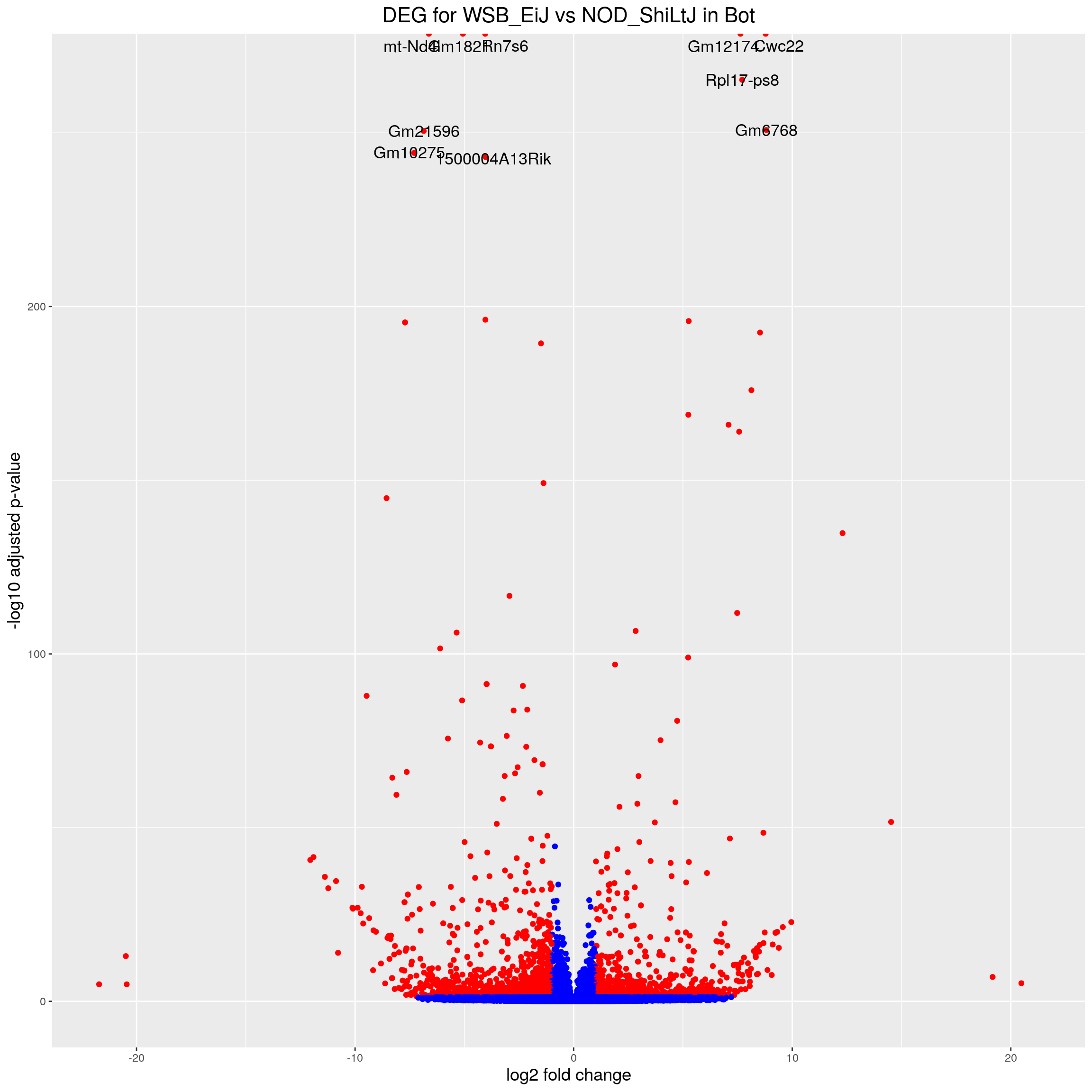
| Version | Author | Date |
|---|---|---|
| 414688f | xhyuo | 2021-08-09 |
#heatmap
# Extract normalized expression for significant genes fdr < 0.05 & abs(log2FoldChange) >= 1)
normalized_counts_sig.strain.in.Bot <- normalized_counts %>%
filter(gene %in% rownames(subset(resSig.strain.in.Bot, padj < 0.05 & abs(log2FoldChange) >= 1))) %>%
dplyr::select(-1) %>%
dplyr::select(contains("Bot"))
### Set a color palette
heat_colors <- brewer.pal(6, "YlOrRd")
#annotation
df <- as.data.frame(colData(ddsMat)[,c("Strain","Tissue")]) %>%
filter(Tissue == "Bot")
### Run pheatmap using the metadata data frame for the annotation
sig.strain.in.Bot.plot <- pheatmap(as.matrix(normalized_counts_sig.strain.in.Bot),
color = heat_colors,
cluster_rows = T,
show_rownames = F,
annotation_col = df,
annotation_colors = list(Strain = c(NOD_ShiLtJ = "#0064C9",
WSB_EiJ ="#B10DC9"),
Tissue = c(Bot = "#96ca00",
NTS = "#ff9289")),
border_color = NA,
fontsize = 10,
scale = "row",
fontsize_row = 10,
height = 20,
legend = FALSE,
annotation_legend = FALSE,
annotation_names_col = FALSE
#main = "Heatmap of the top DEGs in WSB_EiJ vs NOD_ShiLtJ in Bot (fdr < 0.05 & abs(log2FoldChange) >= 1)"
)
sig.strain.in.Bot.plot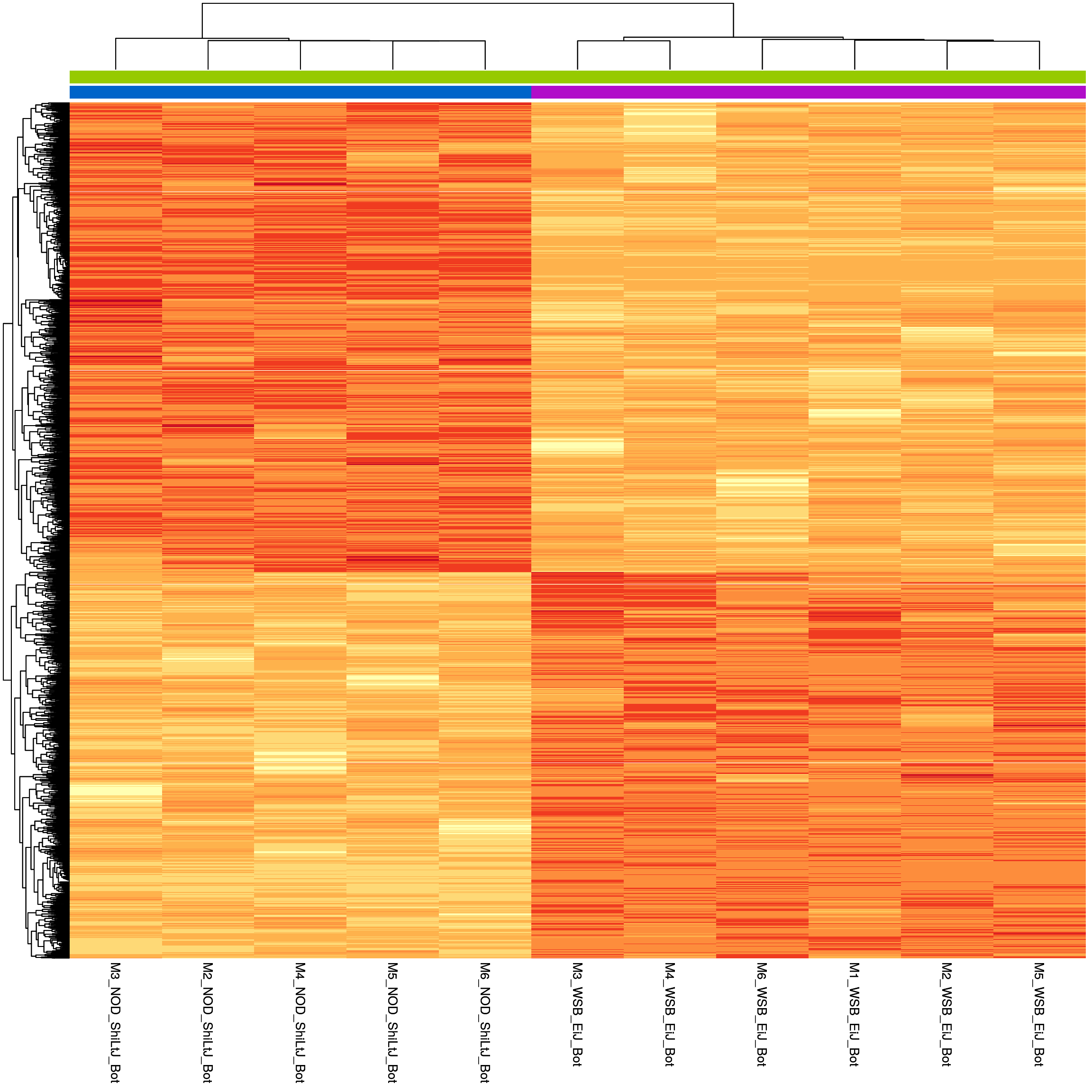
| Version | Author | Date |
|---|---|---|
| 414688f | xhyuo | 2021-08-09 |
#enrichment analysis for res.tab.strain.in.Bot-------
dbs <- c("WikiPathways_2019_Mouse",
         "GO_Biological_Process_2021",
         "GO_Cellular_Component_2021",
         "GO_Molecular_Function_2021",
         "KEGG_2019_Mouse",
         "Mouse_Gene_Atlas",
         "MGI_Mammalian_Phenotype_Level_4_2019")

#results (fdr < 0.05)------
resSig.strain.in.Bot.tab <- resSig.strain.in.Bot %>%
  data.frame() %>%
  rownames_to_column(var="target_id") %>%
  as_tibble() %>%
  left_join(genes)
Joining, by = "target_id"#up-regulated genes WSB_EiJ vs NOD_ShiLtJ in Bot ---------------------------
up.genes <- resSig.strain.in.Bot.tab %>%
filter(log2FoldChange > 0) %>%
pull(SYMBOL)
#up-regulated genes enrichment
up.genes.enriched <- enrichr(as.character(na.omit(up.genes)), dbs)Uploading data to Enrichr... Done.
Querying WikiPathways_2019_Mouse... Done.
Querying GO_Biological_Process_2021... Done.
Querying GO_Cellular_Component_2021... Done.
Querying GO_Molecular_Function_2021... Done.
Querying KEGG_2019_Mouse... Done.
Querying Mouse_Gene_Atlas... Done.
Querying MGI_Mammalian_Phenotype_Level_4_2019... Done.
Parsing results... Done.for (j in 1:length(up.genes.enriched)){
up.genes.enriched[[j]] <- cbind(data.frame(Library = names(up.genes.enriched)[j]),up.genes.enriched[[j]])
}
up.genes.enriched <- do.call(rbind.data.frame, up.genes.enriched) %>%
filter(Adjusted.P.value <= 0.05) %>%
mutate(logpvalue = -log10(P.value)) %>%
arrange(desc(logpvalue))
#display up.genes.enriched
DT::datatable(up.genes.enriched,
filter = list(position = 'top', clear = FALSE),
extensions = 'Buttons',
options = list(dom = 'Blfrtip',
buttons = c('csv', 'excel'),
lengthMenu = list(c(10,25,50,-1),c(10,25,50,"All")),
pageLength = 40,
scrollY = "300px",
scrollX = "40px")
)#barpot
up.genes.enriched.plot.in.Bot <- up.genes.enriched %>%
filter(Adjusted.P.value <= 0.01) %>%
mutate(Term = fct_reorder(Term, -logpvalue)) %>%
ggplot(data = ., aes(x = Term, y = logpvalue, fill = Library, label = Overlap)) +
geom_bar(stat = "identity") +
geom_text(position = position_dodge(width = 0.9),
hjust = 0) +
theme_bw() +
ylab("-log(p.value)") +
xlab("") +
ggtitle("Enrichment of up-regulated genes for WSB_EiJ vs NOD_ShiLtJ \nin Bot (Adjusted.P.value <= 0.01)") +
theme(plot.background = element_blank() ,
panel.border = element_blank(),
panel.background = element_blank(),
#legend.position = "none",
plot.title = element_text(hjust = 0),
panel.grid.major = element_blank(),
panel.grid.minor = element_blank()) +
theme(axis.line = element_line(color = 'black')) +
theme(axis.title.x = element_text(size = 12, vjust=-0.5)) +
theme(axis.title.y = element_text(size = 12, vjust= 1.0)) +
theme(axis.text = element_text(size = 12)) +
theme(plot.title = element_text(size = 12)) +
coord_flip()
up.genes.enriched.plot.in.Bot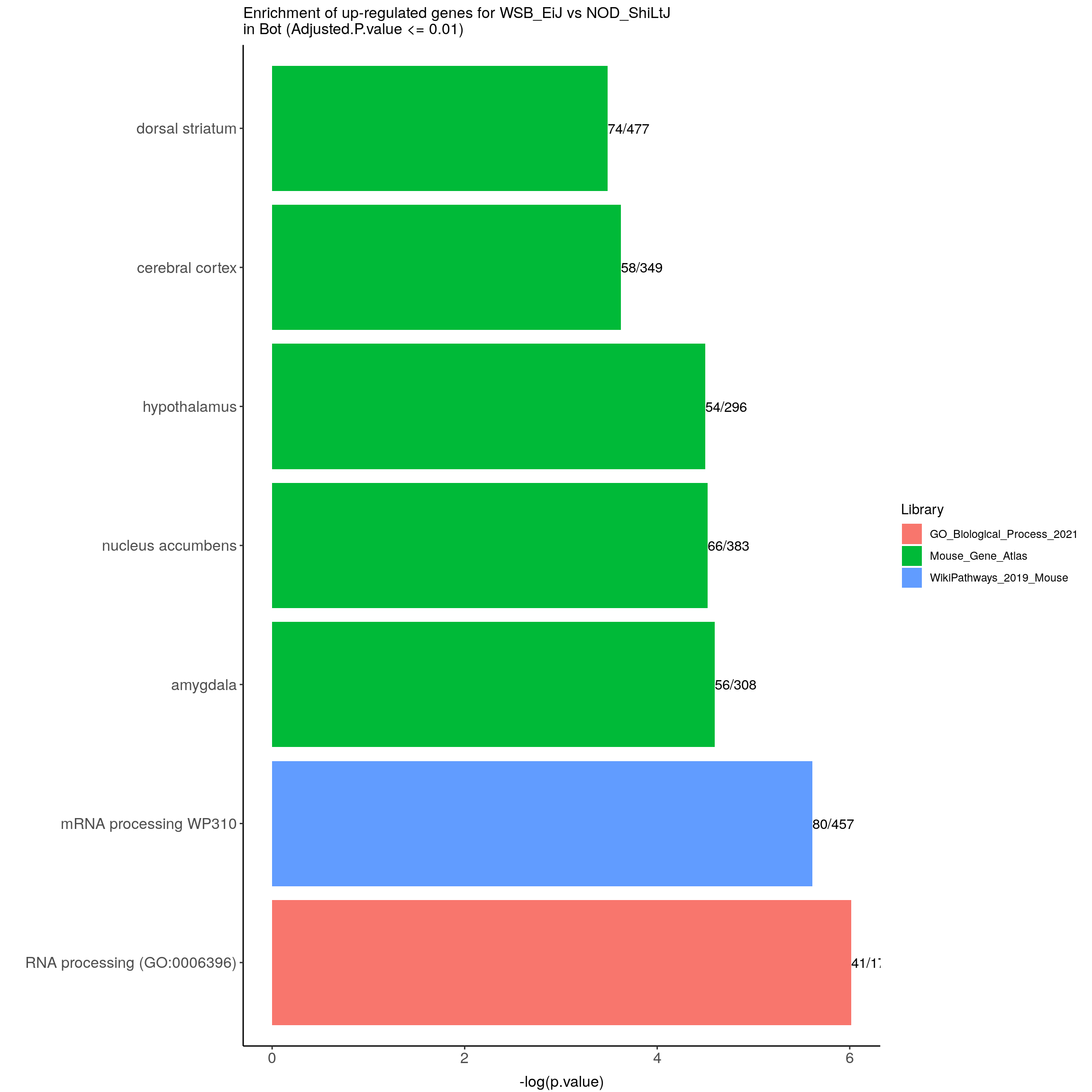
| Version | Author | Date |
|---|---|---|
| 414688f | xhyuo | 2021-08-09 |
#down-regulated genes WSB_EiJ vs NOD_ShiLtJ in Bot---------------------------
down.genes <- resSig.strain.in.Bot.tab %>%
  filter(log2FoldChange < 0) %>%
  pull(SYMBOL)
#down-regulated genes enrichment
down.genes.enriched <- enrichr(as.character(na.omit(down.genes)), dbs)
Uploading data to Enrichr... Done.
Querying WikiPathways_2019_Mouse... Done.
Querying GO_Biological_Process_2021... Done.
Querying GO_Cellular_Component_2021... Done.
Querying GO_Molecular_Function_2021... Done.
Querying KEGG_2019_Mouse... Done.
Querying Mouse_Gene_Atlas... Done.
Querying MGI_Mammalian_Phenotype_Level_4_2019... Done.
Parsing results... Done.for (j in 1:length(down.genes.enriched)){
down.genes.enriched[[j]] <- cbind(data.frame(Library = names(down.genes.enriched)[j]),down.genes.enriched[[j]])
}
down.genes.enriched <- do.call(rbind.data.frame, down.genes.enriched) %>%
filter(Adjusted.P.value <= 0.05) %>%
mutate(logpvalue = -log10(P.value)) %>%
arrange(desc(logpvalue))
#display down.genes.enriched
DT::datatable(down.genes.enriched,
filter = list(position = 'top', clear = FALSE),
extensions = 'Buttons',
options = list(dom = 'Blfrtip',
buttons = c('csv', 'excel'),
lengthMenu = list(c(10,25,50,-1),c(10,25,50,"All")),
pageLength = 40,
scrollY = "300px",
scrollX = "40px")
)#barpot
down.genes.enriched.plot.in.Bot <- down.genes.enriched %>%
filter(Adjusted.P.value <= 0.001) %>%
mutate(Term = fct_reorder(Term, -logpvalue)) %>%
ggplot(data = ., aes(x = Term, y = logpvalue, fill = Library, label = Overlap)) +
geom_bar(stat = "identity") +
geom_text(position = position_dodge(width = 0.9),
hjust = 0) +
theme_bw() +
ylab("-log(p.value)") +
xlab("") +
ggtitle("Enrichment of down-regulated genes for WSB_EiJ vs NOD_ShiLtJ \nin Bot (Adjusted.P.value <= 0.001)") +
theme(plot.background = element_blank() ,
panel.border = element_blank(),
panel.background = element_blank(),
#legend.position = "none",
plot.title = element_text(hjust = 0),
panel.grid.major = element_blank(),
panel.grid.minor = element_blank()) +
theme(axis.line = element_line(color = 'black')) +
theme(axis.title.x = element_text(size = 12, vjust=-0.5)) +
theme(axis.title.y = element_text(size = 12, vjust= 1.0)) +
theme(axis.text = element_text(size = 12)) +
theme(plot.title = element_text(size = 12)) +
coord_flip()
down.genes.enriched.plot.in.Bot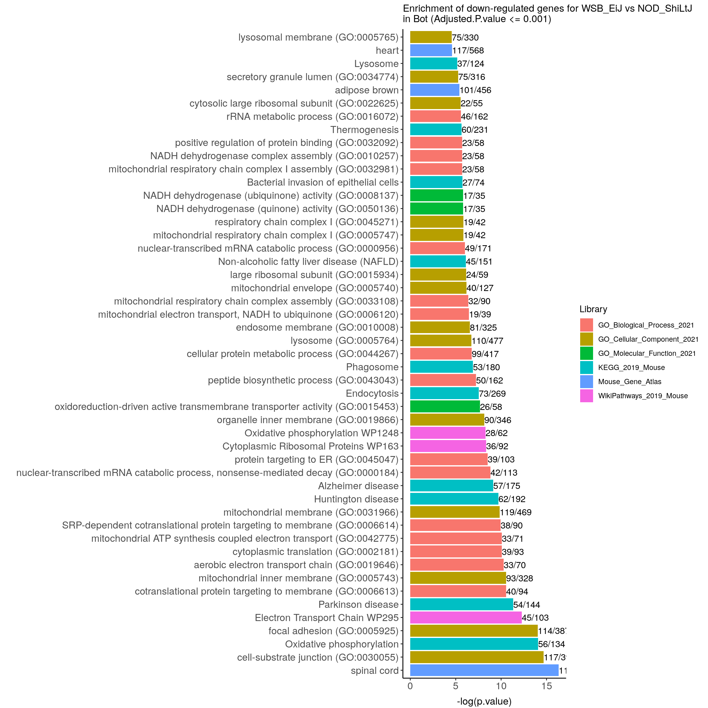
| Version | Author | Date |
|---|---|---|
| 414688f | xhyuo | 2021-08-09 |
The effect of Strain in NTS with one outlier removed
#This is, by definition, the main effect plus the interaction term
#Building the results table
res.tab.strain.in.NTS <- results(res, list(c("Strain_WSB_EiJ_vs_NOD_ShiLtJ",
                                             "TissueNTS.StrainWSB_EiJ")), alpha = 0.05)
summary(res.tab.strain.in.NTS)
out of 78609 with nonzero total read count
adjusted p-value < 0.05
LFC > 0 (up) : 1813, 2.3%
LFC < 0 (down) : 2638, 3.4%
outliers [1] : 477, 0.61%
low counts [2] : 16438, 21%
(mean count < 3)
[1] see 'cooksCutoff' argument of ?results
[2] see 'independentFiltering' argument of ?resultstable(res.tab.strain.in.NTS$padj < 0.05)
FALSE TRUE
57243 4451 #We subset the results table to these genes and then sort it by the log2 fold change estimate to get the significant genes with the strongest down-regulation:
resSig.strain.in.NTS <- subset(res.tab.strain.in.NTS, padj < 0.05)
head(resSig.strain.in.NTS[order(resSig.strain.in.NTS$log2FoldChange), ])log2 fold change (MLE): Strain_WSB_EiJ_vs_NOD_ShiLtJ+TissueNTS.StrainWSB_EiJ effect
Wald test p-value: Strain_WSB_EiJ_vs_NOD_ShiLtJ+TissueNTS.StrainWSB_EiJ effect
DataFrame with 6 rows and 6 columns
baseMean log2FoldChange lfcSE stat pvalue
<numeric> <numeric> <numeric> <numeric> <numeric>
ENSMUST00000165515 5.18071 -26.7060 4.20778 -6.34682 2.19810e-10
ENSMUST00000103071 67.73255 -25.2062 3.44219 -7.32273 2.42984e-13
ENSMUST00000147081 10.02322 -21.5648 2.83501 -7.60659 2.81423e-14
ENSMUST00000148624 6.41829 -21.2253 3.31507 -6.40266 1.52694e-10
ENSMUST00000176612 8.81584 -20.0153 2.50878 -7.97809 1.48615e-15
ENSMUST00000174728 375.36346 -12.0659 0.92237 -13.08138 4.20730e-39
padj
<numeric>
ENSMUST00000165515 2.30628e-08
ENSMUST00000103071 3.65626e-11
ENSMUST00000147081 4.53319e-12
ENSMUST00000148624 1.65559e-08
ENSMUST00000176612 2.66531e-13
ENSMUST00000174728 2.98351e-36# with the strongest up-regulation:
head(resSig.strain.in.NTS[order(resSig.strain.in.NTS$log2FoldChange, decreasing = TRUE), ])log2 fold change (MLE): Strain_WSB_EiJ_vs_NOD_ShiLtJ+TissueNTS.StrainWSB_EiJ effect
Wald test p-value: Strain_WSB_EiJ_vs_NOD_ShiLtJ+TissueNTS.StrainWSB_EiJ effect
DataFrame with 6 rows and 6 columns
baseMean log2FoldChange lfcSE stat pvalue
<numeric> <numeric> <numeric> <numeric> <numeric>
ENSMUST00000123819 28.8648 22.18995 1.843103 12.0395 2.20412e-33
ENSMUST00000111824 3977.3833 15.30673 0.838418 18.2567 1.83073e-74
ENSMUST00000084007 2114.2919 13.15201 0.825916 15.9242 4.30817e-57
ENSMUST00000077016 125.1810 10.50601 0.884441 11.8787 1.52733e-32
ENSMUST00000194648 98.4819 10.10871 0.856897 11.7969 4.05064e-32
ENSMUST00000112797 83.2286 9.80282 0.865490 11.3263 9.72026e-30
padj
<numeric>
ENSMUST00000123819 1.32020e-30
ENSMUST00000111824 2.82363e-71
ENSMUST00000084007 4.83251e-54
ENSMUST00000077016 8.80629e-30
ENSMUST00000194648 2.27182e-29
ENSMUST00000112797 4.87546e-27#Visualization for res.tab.strain.in.NTS------
#Volcano plot
## Obtain logical vector regarding whether padj values are less than 0.05
threshold_OE <- (res.tab.strain.in.NTS$padj < 0.05 & !is.na(res.tab.strain.in.NTS$padj) & abs(res.tab.strain.in.NTS$log2FoldChange) >= 1)
## Determine the number of TRUE values
length(which(threshold_OE))[1] 2167## Add logical vector as a column (threshold) to the res.tab.strain.in.NTS
res.tab.strain.in.NTS$threshold <- threshold_OE
## Sort by ordered padj
res.tab.strain.in.NTS_ordered <- res.tab.strain.in.NTS %>%
data.frame() %>%
rownames_to_column(var="target_id") %>%
arrange(padj) %>%
mutate(genelabels = "") %>%
as_tibble() %>%
left_join(genes)Joining, by = "target_id"## Create a column to indicate which genes to label
res.tab.strain.in.NTS_ordered$genelabels[1:10] <- res.tab.strain.in.NTS_ordered$SYMBOL[1:10]
#display res.tab.strain.in.NTS_ordered
DT::datatable(res.tab.strain.in.NTS_ordered[(res.tab.strain.in.NTS_ordered$padj < 0.05 & !is.na(res.tab.strain.in.NTS_ordered$padj)), ],
filter = list(position = 'top', clear = FALSE),
extensions = 'Buttons',
options = list(dom = 'Blfrtip',
buttons = c('csv', 'excel'),
lengthMenu = list(c(10,25,50,-1),c(10,25,50,"All")),
pageLength = 40,
scrollY = "300px",
scrollX = "40px"),
caption = htmltools::tags$caption(style = 'caption-side: top; text-align: left; color:black; font-size:200% ;','DET for WSB_EiJ vs NOD_ShiLtJ in NTS (fdr < 0.05)'))Warning in instance$preRenderHook(instance): It seems your data is too big
for client-side DataTables. You may consider server-side processing: https://
rstudio.github.io/DT/server.htmlwrite.csv(res.tab.strain.in.NTS_ordered[(res.tab.strain.in.NTS_ordered$padj < 0.05 & !is.na(res.tab.strain.in.NTS_ordered$padj)), ],
file = "data/rnaseq/DET_WSB_vs_NOD_in_NTS_fdr_0.05_with_one_outlier_removed.csv",
row.names = F, quote = F)
#Volcano plot
volcano.plot.strain.in.NTS <- ggplot(res.tab.strain.in.NTS_ordered) +
  geom_point(aes(x = log2FoldChange, y = -log10(padj), colour = threshold)) +
  scale_color_manual(values=c("blue", "red")) +
  geom_text_repel(aes(x = log2FoldChange, y = -log10(padj),
                      label = genelabels,
                      size = 3.5)) +
  ggtitle("DEG for WSB_EiJ vs NOD_ShiLtJ in NTS") +
  xlab("log2 fold change") +
  ylab("-log10 adjusted p-value") +
  theme(legend.position = "none",
        plot.title = element_text(size = rel(1.5), hjust = 0.5),
        axis.title = element_text(size = rel(1.25)))
print(volcano.plot.strain.in.NTS)
Warning: Removed 17055 rows containing missing values (geom_point).Warning: Removed 17055 rows containing missing values (geom_text_repel).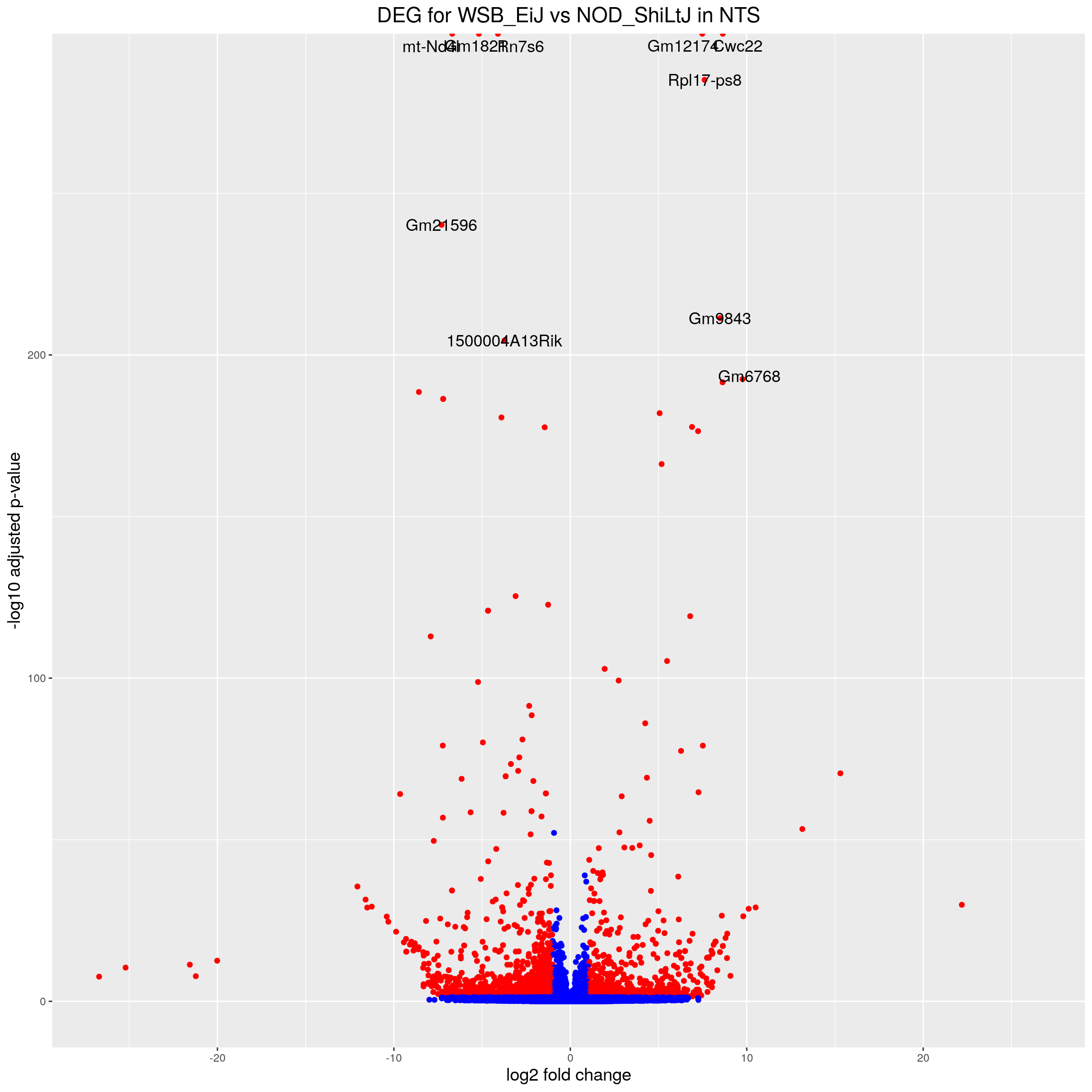
| Version | Author | Date |
|---|---|---|
| 414688f | xhyuo | 2021-08-09 |
#heatmap
# Extract normalized expression for significant genes fdr < 0.05 & abs(log2FoldChange) >= 1)
normalized_counts_sig.strain.in.NTS <- normalized_counts %>%
filter(gene %in% rownames(subset(resSig.strain.in.NTS, padj < 0.05 & abs(log2FoldChange) >= 1))) %>%
dplyr::select(-1) %>%
dplyr::select(contains("NTS")) %>%
dplyr::select(-M6_WSB_EiJ_NTS)
### Set a color palette
heat_colors <- brewer.pal(6, "YlOrRd")
#annotation
df <- as.data.frame(colData(ddsMat)[,c("Strain","Tissue")]) %>%
filter(Tissue == "NTS") %>%
filter(rownames(.) != "M6_WSB_EiJ_NTS")
### Run pheatmap using the metadata data frame for the annotation
sig.strain.in.NTS.plot <- pheatmap(as.matrix(normalized_counts_sig.strain.in.NTS),
color = heat_colors,
cluster_rows = T,
show_rownames = F,
annotation_col = df,
annotation_colors = list(Strain = c(NOD_ShiLtJ = "#0064C9",
WSB_EiJ ="#B10DC9"),
Tissue = c(Bot = "#96ca00",
NTS = "#ff9289")),
border_color = NA,
fontsize = 10,
scale = "row",
fontsize_row = 10,
height = 20
#legend = FALSE,
#annotation_legend = FALSE,
#annotation_names_col = FALSE,
#main = "Heatmap of the top DEGs in WSB_EiJ vs NOD_ShiLtJ in NTS (fdr < 0.05 & abs(log2FoldChange) >= 1)"
)
sig.strain.in.NTS.plot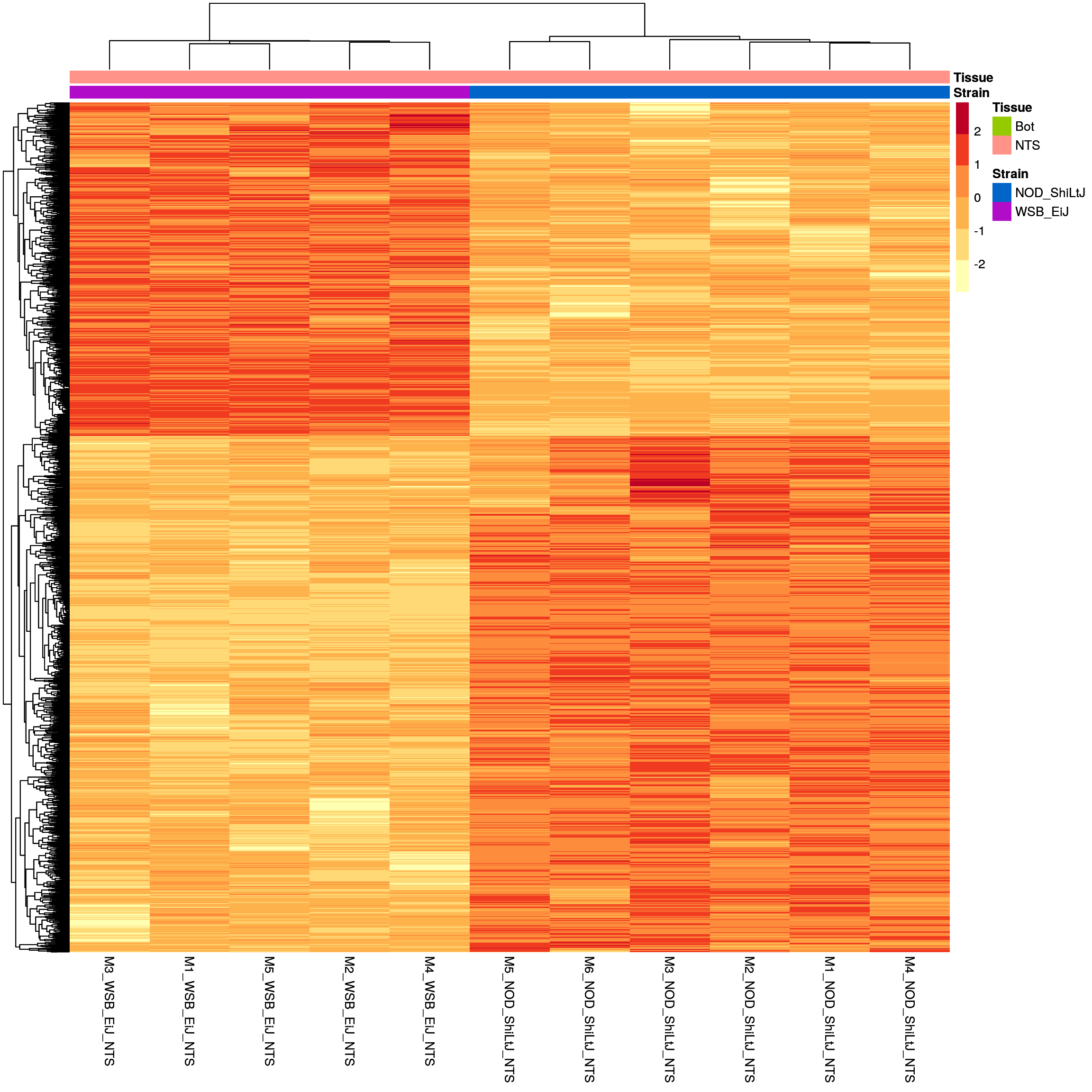
| Version | Author | Date |
|---|---|---|
| 414688f | xhyuo | 2021-08-09 |
#plot sig.strain.in.Bot.plot and sig.strain.in.NTS.plot together-------
ht.map2.plot = plot_grid(as.grob(sig.strain.in.Bot.plot),
          as.grob(sig.strain.in.NTS.plot),
          align = "h", rel_widths = c(1, 1.3),
          labels = c('A', 'B'))
#add title
# now add the title
title <- ggdraw() +
  draw_label(
    "Heatmap of the top DEGs in WSB_EiJ vs NOD_ShiLtJ in Bot and NTS, respectively (fdr < 0.05 & abs(log2FoldChange) >= 1)",
    fontface = 'bold',
    x = 0,
    hjust = 0
  )
plot_grid(
  title,
  ht.map2.plot,
  ncol = 1,
  # rel_heights values control vertical title margins
  rel_heights = c(0.1, 1)
)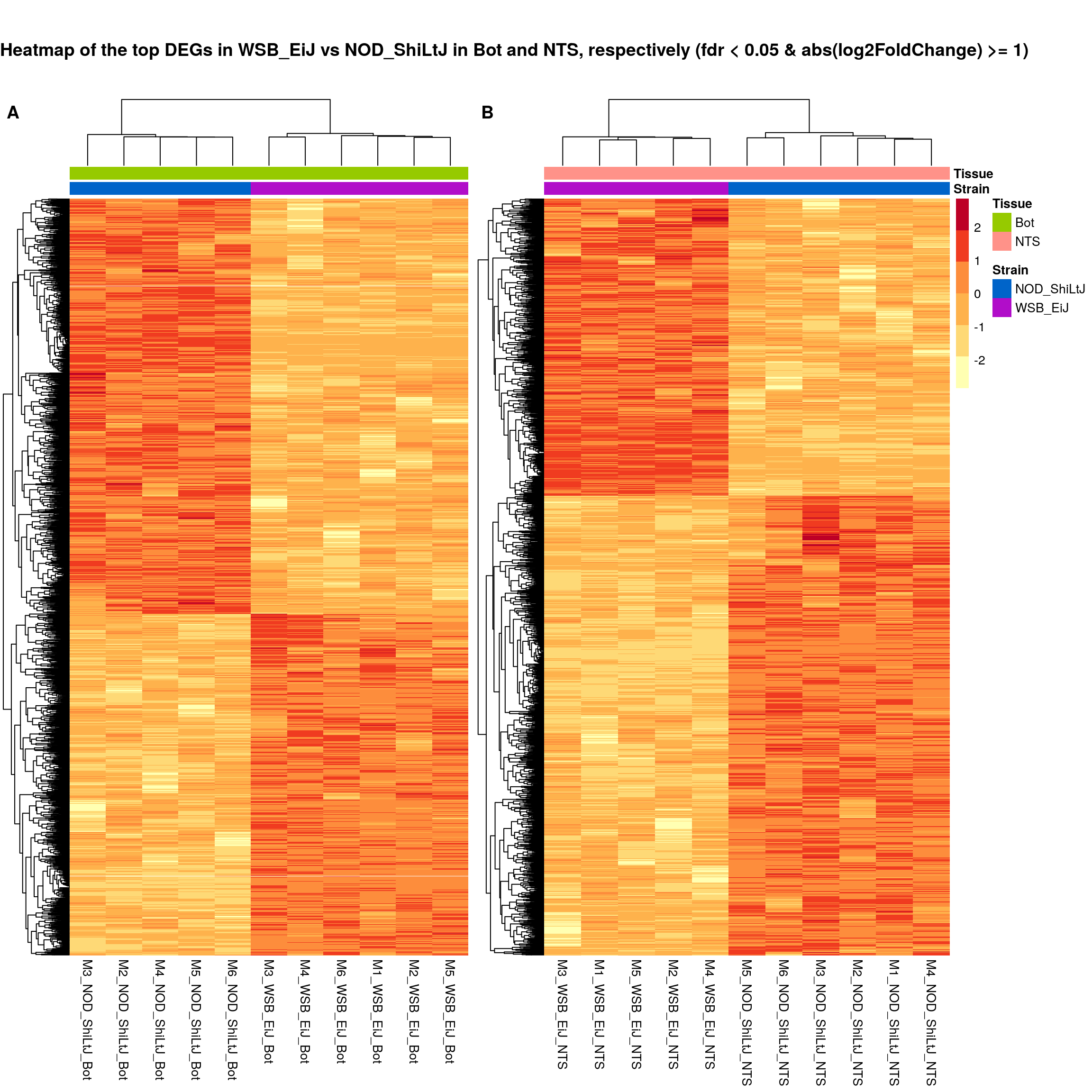
| Version | Author | Date |
|---|---|---|
| 414688f | xhyuo | 2021-08-09 |
#logFC heatmap on both Bot and NTS top DEGs-----
restop.tab.in.Bot.NTS <- full_join(res.tab.strain.in.Bot_ordered,
                                   res.tab.strain.in.NTS_ordered,
                                   by = c("ENSEMBL", "SYMBOL")) %>%
  filter((ENSEMBL %in% res.tab.strain.in.Bot_ordered$ENSEMBL[1:30]) | (ENSEMBL %in% res.tab.strain.in.NTS_ordered$ENSEMBL[1:30]))

restop.tab.in.Bot.NTS.mat <- as.matrix(restop.tab.in.Bot.NTS[, c("log2FoldChange.x", "log2FoldChange.y")])
rownames(restop.tab.in.Bot.NTS.mat) <-
  ifelse(is.na(restop.tab.in.Bot.NTS$SYMBOL),
         restop.tab.in.Bot.NTS$ENSEMBL,
         paste0(restop.tab.in.Bot.NTS$SYMBOL,":", restop.tab.in.Bot.NTS$ENSEMBL))
colnames(restop.tab.in.Bot.NTS.mat) <- c("Bot", "NTS")

#heatmap
### Run pheatmap using the metadata data frame for the annotation
pheatmap(restop.tab.in.Bot.NTS.mat,
         color = colorpanel(1000, "blue", "white", "red"),
         cluster_rows  = T,
         show_rownames = T,
         border_color  = NA,
         fontsize = 10,
         fontsize_row = 8,
         height = 25,
         main = "Heatmap of log2FoldChange for the top 30 DEGs in Bot and NTS")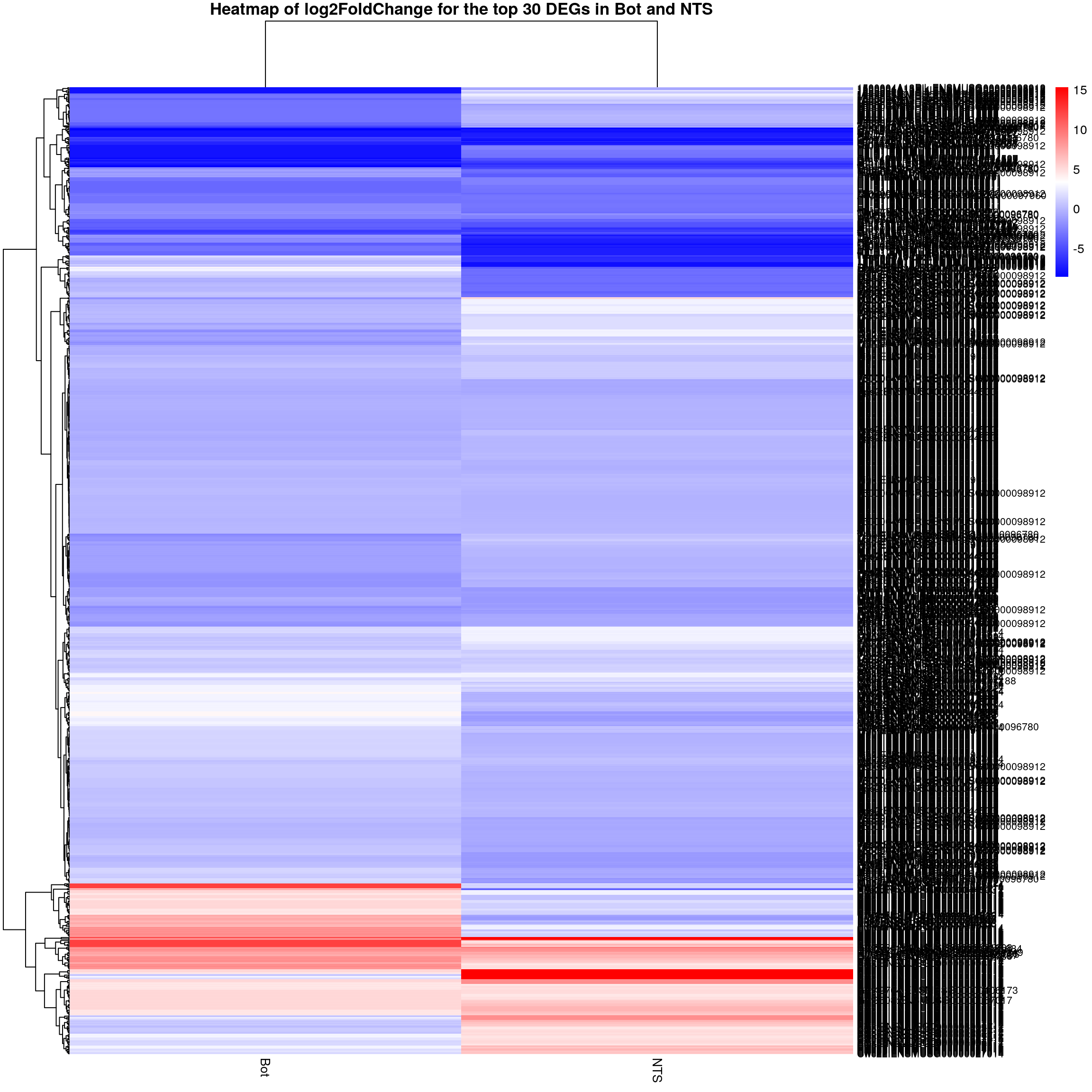
| Version | Author | Date |
|---|---|---|
| 414688f | xhyuo | 2021-08-09 |
#enrichment analysis for res.tab.strain.in.NTS-------
dbs <- c("WikiPathways_2019_Mouse",
         "GO_Biological_Process_2021",
         "GO_Cellular_Component_2021",
         "GO_Molecular_Function_2021",
         "KEGG_2019_Mouse",
         "Mouse_Gene_Atlas",
         "MGI_Mammalian_Phenotype_Level_4_2019")

#results (fdr < 0.05)------
resSig.strain.in.NTS.tab <- resSig.strain.in.NTS %>%
  data.frame() %>%
  rownames_to_column(var="target_id") %>%
  as_tibble() %>%
  left_join(genes)
Joining, by = "target_id"#up-regulated genes WSB_EiJ vs NOD_ShiLtJ in NTS ---------------------------
up.genes <- resSig.strain.in.NTS.tab %>%
filter(log2FoldChange > 0) %>%
pull(SYMBOL)
#up-regulated genes enrichment
up.genes.enriched <- enrichr(as.character(na.omit(up.genes)), dbs)Uploading data to Enrichr... Done.
Querying WikiPathways_2019_Mouse... Done.
Querying GO_Biological_Process_2021... Done.
Querying GO_Cellular_Component_2021... Done.
Querying GO_Molecular_Function_2021... Done.
Querying KEGG_2019_Mouse... Done.
Querying Mouse_Gene_Atlas... Done.
Querying MGI_Mammalian_Phenotype_Level_4_2019... Done.
Parsing results... Done.for (j in 1:length(up.genes.enriched)){
up.genes.enriched[[j]] <- cbind(data.frame(Library = names(up.genes.enriched)[j]),up.genes.enriched[[j]])
}
up.genes.enriched <- do.call(rbind.data.frame, up.genes.enriched) %>%
filter(Adjusted.P.value <= 0.5) %>%
mutate(logpvalue = -log10(P.value)) %>%
arrange(desc(logpvalue))
#display up.genes.enriched
DT::datatable(up.genes.enriched,
filter = list(position = 'top', clear = FALSE),
extensions = 'Buttons',
options = list(dom = 'Blfrtip',
buttons = c('csv', 'excel'),
lengthMenu = list(c(10,25,50,-1),c(10,25,50,"All")),
pageLength = 40,
scrollY = "300px",
scrollX = "40px")
)#barpot
up.genes.enriched.plot.in.NTS <- up.genes.enriched %>%
filter(Adjusted.P.value <= 0.5) %>%
mutate(Term = fct_reorder(Term, -logpvalue)) %>%
ggplot(data = ., aes(x = Term, y = logpvalue, fill = Library, label = Overlap)) +
geom_bar(stat = "identity") +
geom_text(position = position_dodge(width = 0.9),
hjust = 0) +
theme_bw() +
ylab("-log(p.value)") +
xlab("") +
ggtitle("Enrichment of up-regulated genes for WSB_EiJ vs NOD_ShiLtJ \nin NTS (Adjusted.P.value <= 0.5)") +
theme(plot.background = element_blank() ,
panel.border = element_blank(),
panel.background = element_blank(),
#legend.position = "none",
plot.title = element_text(hjust = 0),
panel.grid.major = element_blank(),
panel.grid.minor = element_blank()) +
theme(axis.line = element_line(color = 'black')) +
theme(axis.title.x = element_text(size = 12, vjust=-0.5)) +
theme(axis.title.y = element_text(size = 12, vjust= 1.0)) +
theme(axis.text = element_text(size = 12)) +
theme(plot.title = element_text(size = 12)) +
coord_flip()
up.genes.enriched.plot.in.NTS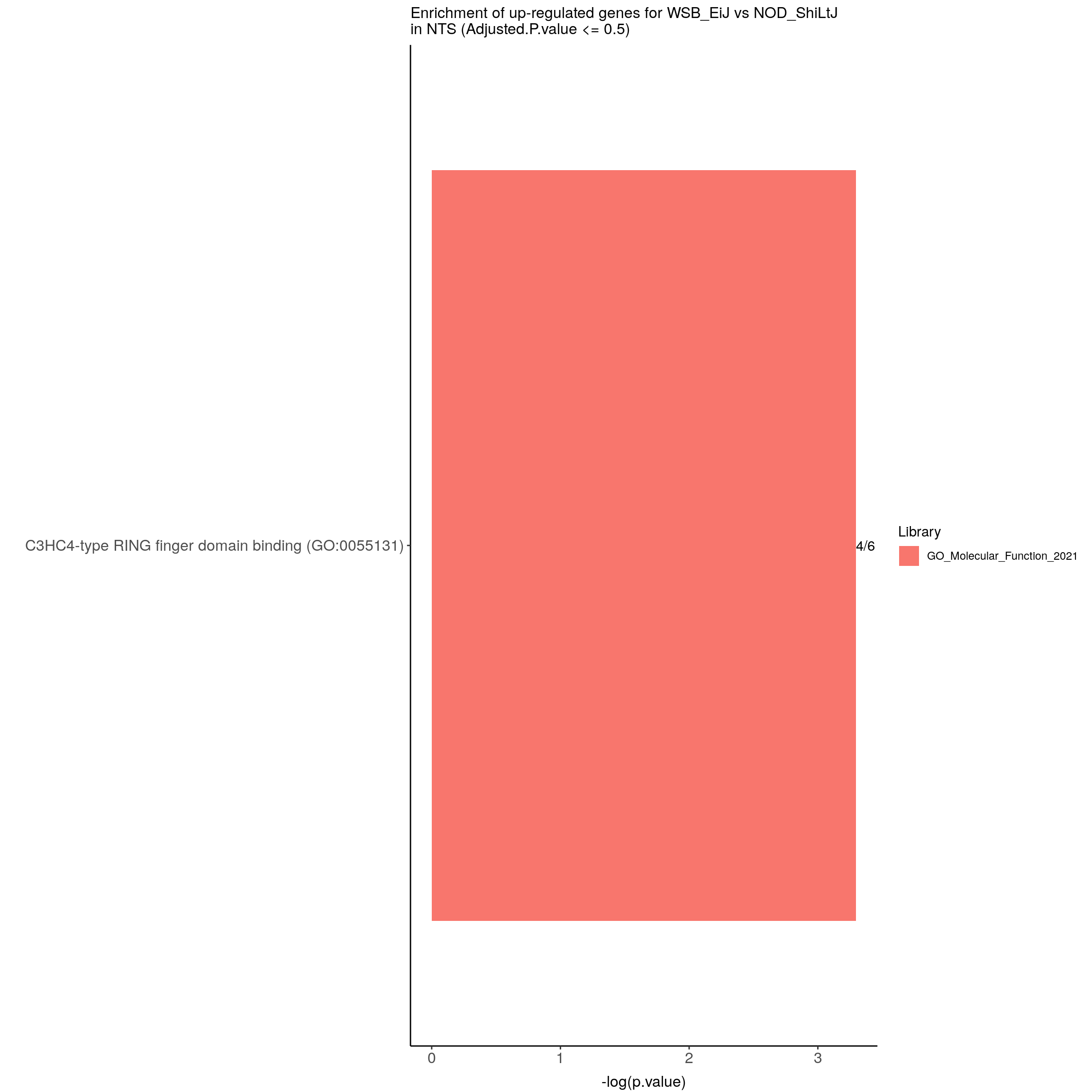
| Version | Author | Date |
|---|---|---|
| 414688f | xhyuo | 2021-08-09 |
#down-regulated genes WSB_EiJ vs NOD_ShiLtJ in NTS---------------------------
down.genes <- resSig.strain.in.NTS.tab %>%
  filter(log2FoldChange < 0) %>%
  pull(SYMBOL)
#down-regulated genes enrichment
down.genes.enriched <- enrichr(as.character(na.omit(down.genes)), dbs)
Uploading data to Enrichr... Done.
Querying WikiPathways_2019_Mouse... Done.
Querying GO_Biological_Process_2021... Done.
Querying GO_Cellular_Component_2021... Done.
Querying GO_Molecular_Function_2021... Done.
Querying KEGG_2019_Mouse... Done.
Querying Mouse_Gene_Atlas... Done.
Querying MGI_Mammalian_Phenotype_Level_4_2019... Done.
Parsing results... Done.for (j in 1:length(down.genes.enriched)){
down.genes.enriched[[j]] <- cbind(data.frame(Library = names(down.genes.enriched)[j]),down.genes.enriched[[j]])
}
down.genes.enriched <- do.call(rbind.data.frame, down.genes.enriched) %>%
filter(Adjusted.P.value <= 0.05) %>%
mutate(logpvalue = -log10(P.value)) %>%
arrange(desc(logpvalue))
#display down.genes.enriched
DT::datatable(down.genes.enriched,
filter = list(position = 'top', clear = FALSE),
extensions = 'Buttons',
options = list(dom = 'Blfrtip',
buttons = c('csv', 'excel'),
lengthMenu = list(c(10,25,50,-1),c(10,25,50,"All")),
pageLength = 40,
scrollY = "300px",
scrollX = "40px")
)#barpot
down.genes.enriched.plot.in.NTS <- down.genes.enriched %>%
filter(Adjusted.P.value <= 0.001) %>%
mutate(Term = fct_reorder(Term, -logpvalue)) %>%
ggplot(data = ., aes(x = Term, y = logpvalue, fill = Library, label = Overlap)) +
geom_bar(stat = "identity") +
geom_text(position = position_dodge(width = 0.9),
hjust = 0) +
theme_bw() +
ylab("-log(p.value)") +
xlab("") +
ggtitle("Enrichment of down-regulated genes for WSB_EiJ vs NOD_ShiLtJ \nin NTS (Adjusted.P.value <= 0.001)") +
theme(plot.background = element_blank() ,
panel.border = element_blank(),
panel.background = element_blank(),
#legend.position = "none",
plot.title = element_text(hjust = 0),
panel.grid.major = element_blank(),
panel.grid.minor = element_blank()) +
theme(axis.line = element_line(color = 'black')) +
theme(axis.title.x = element_text(size = 12, vjust=-0.5)) +
theme(axis.title.y = element_text(size = 12, vjust= 1.0)) +
theme(axis.text = element_text(size = 12)) +
theme(plot.title = element_text(size = 12)) +
coord_flip()
down.genes.enriched.plot.in.NTS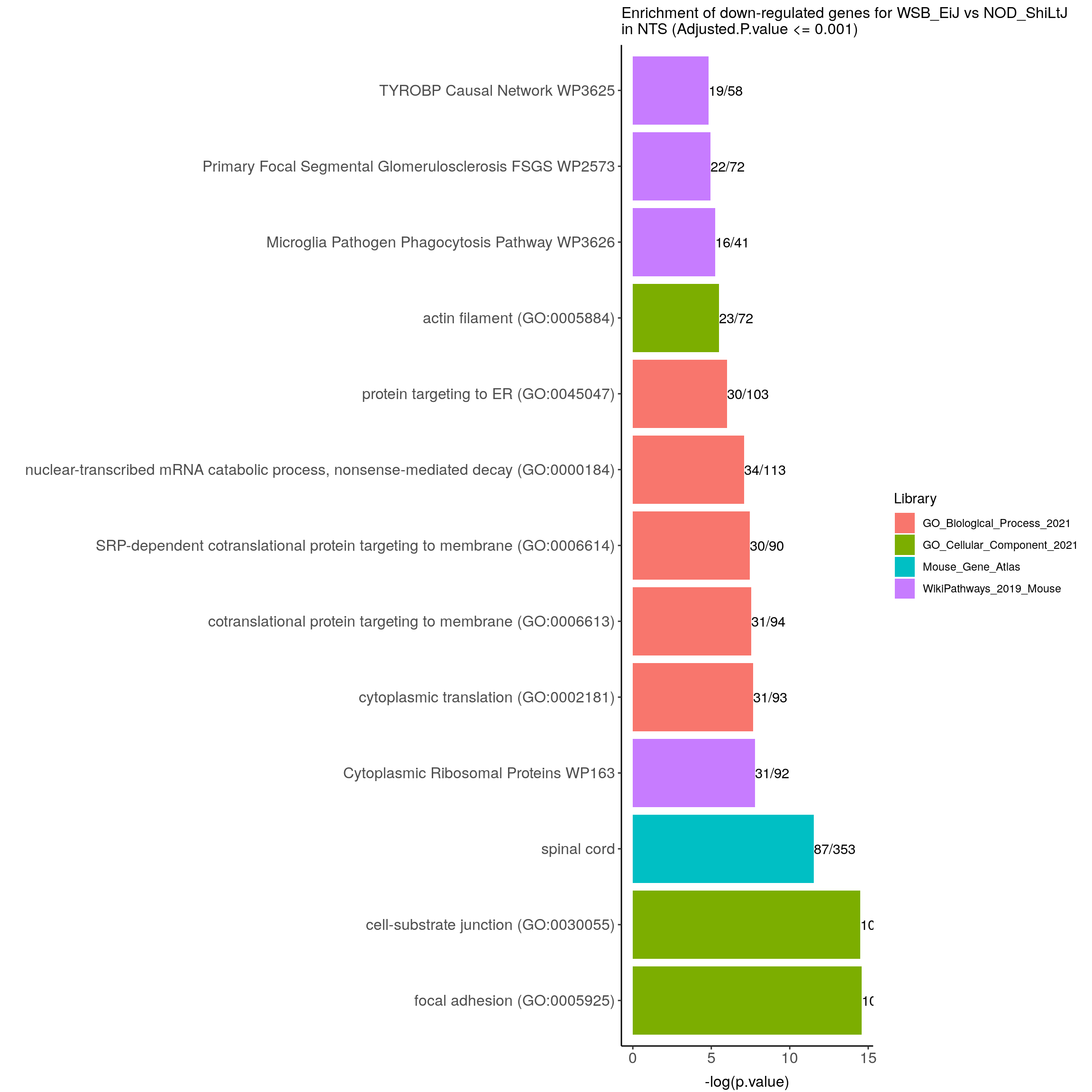
| Version | Author | Date |
|---|---|---|
| 414688f | xhyuo | 2021-08-09 |
sessionInfo()R version 4.0.3 (2020-10-10)
Platform: x86_64-pc-linux-gnu (64-bit)
Running under: Ubuntu 20.04.1 LTS
Matrix products: default
BLAS/LAPACK: /usr/lib/x86_64-linux-gnu/openblas-pthread/libopenblasp-r0.3.8.so
locale:
[1] LC_CTYPE=en_US.UTF-8 LC_NUMERIC=C
[3] LC_TIME=en_US.UTF-8 LC_COLLATE=en_US.UTF-8
[5] LC_MONETARY=en_US.UTF-8 LC_MESSAGES=C
[7] LC_PAPER=en_US.UTF-8 LC_NAME=C
[9] LC_ADDRESS=C LC_TELEPHONE=C
[11] LC_MEASUREMENT=en_US.UTF-8 LC_IDENTIFICATION=C
attached base packages:
[1] parallel stats4 stats graphics grDevices utils datasets
[8] methods base
other attached packages:
[1] annotables_0.1.91 ggplotify_0.0.7
[3] cowplot_1.1.1 enrichR_3.0
[5] DT_0.17 ggrepel_0.9.0
[7] pheatmap_1.0.12 DESeq2_1.30.1
[9] SummarizedExperiment_1.18.2 DelayedArray_0.14.1
[11] matrixStats_0.57.0 GenomicRanges_1.40.0
[13] GenomeInfoDb_1.26.2 RColorBrewer_1.1-2
[15] org.Mm.eg.db_3.11.4 AnnotationDbi_1.52.0
[17] IRanges_2.22.2 S4Vectors_0.26.1
[19] Biobase_2.48.0 BiocGenerics_0.36.0
[21] gplots_3.1.1 Glimma_2.0.0
[23] edgeR_3.32.1 limma_3.46.0
[25] forcats_0.5.0 dplyr_1.0.2
[27] purrr_0.3.4 readr_1.4.0
[29] tidyr_1.1.2 tibble_3.0.4
[31] ggplot2_3.3.3 tidyverse_1.3.0
[33] stringr_1.4.0 workflowr_1.6.2
loaded via a namespace (and not attached):
[1] colorspace_2.0-0 rjson_0.2.20 ellipsis_0.3.1
[4] rprojroot_2.0.2 XVector_0.28.0 fs_1.5.0
[7] rstudioapi_0.13 farver_2.0.3 bit64_4.0.5
[10] fansi_0.4.1 lubridate_1.7.9.2 xml2_1.3.2
[13] splines_4.0.3 geneplotter_1.66.0 knitr_1.30
[16] jsonlite_1.7.2 broom_0.7.3 annotate_1.66.0
[19] dbplyr_2.0.0 BiocManager_1.30.10 compiler_4.0.3
[22] httr_1.4.2 rvcheck_0.1.8 backports_1.2.1
[25] assertthat_0.2.1 Matrix_1.3-2 cli_2.2.0
[28] later_1.1.0.1 htmltools_0.5.1 tools_4.0.3
[31] gtable_0.3.0 glue_1.4.2 GenomeInfoDbData_1.2.4
[34] Rcpp_1.0.5 cellranger_1.1.0 vctrs_0.3.6
[37] crosstalk_1.1.1 xfun_0.20 rvest_0.3.6
[40] lifecycle_0.2.0 gtools_3.8.2 XML_3.99-0.5
[43] zlibbioc_1.36.0 scales_1.1.1 hms_1.0.0
[46] promises_1.1.1 curl_4.3 yaml_2.2.1
[49] memoise_1.1.0 stringi_1.5.3 RSQLite_2.2.2
[52] highr_0.8 genefilter_1.70.0 caTools_1.18.1
[55] BiocParallel_1.22.0 rlang_0.4.10 pkgconfig_2.0.3
[58] bitops_1.0-6 evaluate_0.14 lattice_0.20-41
[61] labeling_0.4.2 htmlwidgets_1.5.3 bit_4.0.4
[64] tidyselect_1.1.0 magrittr_2.0.1 R6_2.5.0
[67] generics_0.1.0 DBI_1.1.0 pillar_1.4.7
[70] haven_2.3.1 whisker_0.4 withr_2.3.0
[73] survival_3.2-7 RCurl_1.98-1.2 modelr_0.1.8
[76] crayon_1.3.4 KernSmooth_2.23-18 rmarkdown_2.6
[79] locfit_1.5-9.4 grid_4.0.3 readxl_1.3.1
[82] blob_1.2.1 git2r_0.28.0 reprex_0.3.0
[85] digest_0.6.27 xtable_1.8-4 httpuv_1.5.5
[88] gridGraphics_0.5-1 munsell_0.5.0 This R Markdown site was created with workflowr