DEG_analysis_GSE100356_pos_neg
Last updated: 2022-10-20
Checks: 7 0
Knit directory: DO_Opioid/
This reproducible R Markdown analysis was created with workflowr (version 1.6.2). The Checks tab describes the reproducibility checks that were applied when the results were created. The Past versions tab lists the development history.
Great! Since the R Markdown file has been committed to the Git repository, you know the exact version of the code that produced these results.
Great job! The global environment was empty. Objects defined in the global environment can affect the analysis in your R Markdown file in unknown ways. For reproduciblity it’s best to always run the code in an empty environment.
The command set.seed(20200504) was run prior to running the code in the R Markdown file. Setting a seed ensures that any results that rely on randomness, e.g. subsampling or permutations, are reproducible.
Great job! Recording the operating system, R version, and package versions is critical for reproducibility.
Nice! There were no cached chunks for this analysis, so you can be confident that you successfully produced the results during this run.
Great job! Using relative paths to the files within your workflowr project makes it easier to run your code on other machines.
Great! You are using Git for version control. Tracking code development and connecting the code version to the results is critical for reproducibility.
The results in this page were generated with repository version ed2a911. See the Past versions tab to see a history of the changes made to the R Markdown and HTML files.
Note that you need to be careful to ensure that all relevant files for the analysis have been committed to Git prior to generating the results (you can use wflow_publish or wflow_git_commit). workflowr only checks the R Markdown file, but you know if there are other scripts or data files that it depends on. Below is the status of the Git repository when the results were generated:
Ignored files:
    Ignored:    .RData
    Ignored:    .Rhistory
    Ignored:    .Rproj.user/
    Ignored:    analysis/Picture1.png

Untracked files:
    Untracked:  Rplot_rz.png
    Untracked:  TIMBR.test.prop.bm.MN.RET.RData
    Untracked:  TIMBR.test.random.RData
    Untracked:  TIMBR.test.rz.transformed_TVb_ml.RData
    Untracked:  analysis/DDO_morphine1_second_set_69k.stdout
    Untracked:  analysis/DO_Fentanyl.R
    Untracked:  analysis/DO_Fentanyl.err
    Untracked:  analysis/DO_Fentanyl.out
    Untracked:  analysis/DO_Fentanyl.sh
    Untracked:  analysis/DO_Fentanyl_69k.R
    Untracked:  analysis/DO_Fentanyl_69k.err
    Untracked:  analysis/DO_Fentanyl_69k.out
    Untracked:  analysis/DO_Fentanyl_69k.sh
    Untracked:  analysis/DO_Fentanyl_Cohort2_gemma.R
    Untracked:  analysis/DO_Fentanyl_Cohort2_mapping.R
    Untracked:  analysis/DO_Fentanyl_Cohort2_mapping.err
    Untracked:  analysis/DO_Fentanyl_Cohort2_mapping.out
    Untracked:  analysis/DO_Fentanyl_Cohort2_mapping.sh
    Untracked:  analysis/DO_Fentanyl_GCTA_herit.R
    Untracked:  analysis/DO_Fentanyl_alternate_metrics_69k.R
    Untracked:  analysis/DO_Fentanyl_alternate_metrics_69k.err
    Untracked:  analysis/DO_Fentanyl_alternate_metrics_69k.out
    Untracked:  analysis/DO_Fentanyl_alternate_metrics_69k.sh
    Untracked:  analysis/DO_Fentanyl_alternate_metrics_array.R
    Untracked:  analysis/DO_Fentanyl_alternate_metrics_array.err
    Untracked:  analysis/DO_Fentanyl_alternate_metrics_array.out
    Untracked:  analysis/DO_Fentanyl_alternate_metrics_array.sh
    Untracked:  analysis/DO_Fentanyl_array.R
    Untracked:  analysis/DO_Fentanyl_array.err
    Untracked:  analysis/DO_Fentanyl_array.out
    Untracked:  analysis/DO_Fentanyl_array.sh
    Untracked:  analysis/DO_Fentanyl_combining2Cohort_gemma.R
    Untracked:  analysis/DO_Fentanyl_combining2Cohort_mapping.R
    Untracked:  analysis/DO_Fentanyl_combining2Cohort_mapping.err
    Untracked:  analysis/DO_Fentanyl_combining2Cohort_mapping.out
    Untracked:  analysis/DO_Fentanyl_combining2Cohort_mapping.sh
    Untracked:  analysis/DO_Fentanyl_combining2Cohort_mapping_CoxPH.R
    Untracked:  analysis/DO_Fentanyl_finalreport_to_plink.sh
    Untracked:  analysis/DO_Fentanyl_gemma.R
    Untracked:  analysis/DO_Fentanyl_gemma.err
    Untracked:  analysis/DO_Fentanyl_gemma.out
    Untracked:  analysis/DO_Fentanyl_gemma.sh
    Untracked:  analysis/DO_morphine1.R
    Untracked:  analysis/DO_morphine1.Rout
    Untracked:  analysis/DO_morphine1.sh
    Untracked:  analysis/DO_morphine1.stderr
    Untracked:  analysis/DO_morphine1.stdout
    Untracked:  analysis/DO_morphine1_SNP.R
    Untracked:  analysis/DO_morphine1_SNP.Rout
    Untracked:  analysis/DO_morphine1_SNP.sh
    Untracked:  analysis/DO_morphine1_SNP.stderr
    Untracked:  analysis/DO_morphine1_SNP.stdout
    Untracked:  analysis/DO_morphine1_combined.R
    Untracked:  analysis/DO_morphine1_combined.Rout
    Untracked:  analysis/DO_morphine1_combined.sh
    Untracked:  analysis/DO_morphine1_combined.stderr
    Untracked:  analysis/DO_morphine1_combined.stdout
    Untracked:  analysis/DO_morphine1_combined_69k.R
    Untracked:  analysis/DO_morphine1_combined_69k.Rout
    Untracked:  analysis/DO_morphine1_combined_69k.sh
    Untracked:  analysis/DO_morphine1_combined_69k.stderr
    Untracked:  analysis/DO_morphine1_combined_69k.stdout
    Untracked:  analysis/DO_morphine1_combined_69k_m2.R
    Untracked:  analysis/DO_morphine1_combined_69k_m2.Rout
    Untracked:  analysis/DO_morphine1_combined_69k_m2.sh
    Untracked:  analysis/DO_morphine1_combined_69k_m2.stderr
    Untracked:  analysis/DO_morphine1_combined_69k_m2.stdout
    Untracked:  analysis/DO_morphine1_combined_weight_DOB.R
    Untracked:  analysis/DO_morphine1_combined_weight_DOB.Rout
    Untracked:  analysis/DO_morphine1_combined_weight_DOB.err
    Untracked:  analysis/DO_morphine1_combined_weight_DOB.out
    Untracked:  analysis/DO_morphine1_combined_weight_DOB.sh
    Untracked:  analysis/DO_morphine1_combined_weight_DOB.stderr
    Untracked:  analysis/DO_morphine1_combined_weight_DOB.stdout
    Untracked:  analysis/DO_morphine1_combined_weight_age.R
    Untracked:  analysis/DO_morphine1_combined_weight_age.err
    Untracked:  analysis/DO_morphine1_combined_weight_age.out
    Untracked:  analysis/DO_morphine1_combined_weight_age.sh
    Untracked:  analysis/DO_morphine1_combined_weight_age_GAMMT.R
    Untracked:  analysis/DO_morphine1_combined_weight_age_GAMMT.err
    Untracked:  analysis/DO_morphine1_combined_weight_age_GAMMT.out
    Untracked:  analysis/DO_morphine1_combined_weight_age_GAMMT.sh
    Untracked:  analysis/DO_morphine1_combined_weight_age_GAMMT_chr19.R
    Untracked:  analysis/DO_morphine1_combined_weight_age_GAMMT_chr19.err
    Untracked:  analysis/DO_morphine1_combined_weight_age_GAMMT_chr19.out
    Untracked:  analysis/DO_morphine1_combined_weight_age_GAMMT_chr19.sh
    Untracked:  analysis/DO_morphine1_cph.R
    Untracked:  analysis/DO_morphine1_cph.Rout
    Untracked:  analysis/DO_morphine1_cph.sh
    Untracked:  analysis/DO_morphine1_second_set.R
    Untracked:  analysis/DO_morphine1_second_set.Rout
    Untracked:  analysis/DO_morphine1_second_set.sh
    Untracked:  analysis/DO_morphine1_second_set.stderr
    Untracked:  analysis/DO_morphine1_second_set.stdout
    Untracked:  analysis/DO_morphine1_second_set_69k.R
    Untracked:  analysis/DO_morphine1_second_set_69k.Rout
    Untracked:  analysis/DO_morphine1_second_set_69k.sh
    Untracked:  analysis/DO_morphine1_second_set_69k.stderr
    Untracked:  analysis/DO_morphine1_second_set_SNP.R
    Untracked:  analysis/DO_morphine1_second_set_SNP.Rout
    Untracked:  analysis/DO_morphine1_second_set_SNP.sh
    Untracked:  analysis/DO_morphine1_second_set_SNP.stderr
    Untracked:  analysis/DO_morphine1_second_set_SNP.stdout
    Untracked:  analysis/DO_morphine1_second_set_weight_DOB.R
    Untracked:  analysis/DO_morphine1_second_set_weight_DOB.Rout
    Untracked:  analysis/DO_morphine1_second_set_weight_DOB.err
    Untracked:  analysis/DO_morphine1_second_set_weight_DOB.out
    Untracked:  analysis/DO_morphine1_second_set_weight_DOB.sh
    Untracked:  analysis/DO_morphine1_second_set_weight_DOB.stderr
    Untracked:  analysis/DO_morphine1_second_set_weight_DOB.stdout
    Untracked:  analysis/DO_morphine1_second_set_weight_age.R
    Untracked:  analysis/DO_morphine1_second_set_weight_age.Rout
    Untracked:  analysis/DO_morphine1_second_set_weight_age.err
    Untracked:  analysis/DO_morphine1_second_set_weight_age.out
    Untracked:  analysis/DO_morphine1_second_set_weight_age.sh
    Untracked:  analysis/DO_morphine1_second_set_weight_age.stderr
    Untracked:  analysis/DO_morphine1_second_set_weight_age.stdout
    Untracked:  analysis/DO_morphine1_weight_DOB.R
    Untracked:  analysis/DO_morphine1_weight_DOB.sh
    Untracked:  analysis/DO_morphine1_weight_age.R
    Untracked:  analysis/DO_morphine1_weight_age.sh
    Untracked:  analysis/DO_morphine_gemma.R
    Untracked:  analysis/DO_morphine_gemma.err
    Untracked:  analysis/DO_morphine_gemma.out
    Untracked:  analysis/DO_morphine_gemma.sh
    Untracked:  analysis/DO_morphine_gemma_firstmin.R
    Untracked:  analysis/DO_morphine_gemma_firstmin.err
    Untracked:  analysis/DO_morphine_gemma_firstmin.out
    Untracked:  analysis/DO_morphine_gemma_firstmin.sh
    Untracked:  analysis/DO_morphine_gemma_withpermu.R
    Untracked:  analysis/DO_morphine_gemma_withpermu.err
    Untracked:  analysis/DO_morphine_gemma_withpermu.out
    Untracked:  analysis/DO_morphine_gemma_withpermu.sh
    Untracked:  analysis/DO_morphine_gemma_withpermu_firstbatch_min.depression.R
    Untracked:  analysis/DO_morphine_gemma_withpermu_firstbatch_min.depression.err
    Untracked:  analysis/DO_morphine_gemma_withpermu_firstbatch_min.depression.out
    Untracked:  analysis/DO_morphine_gemma_withpermu_firstbatch_min.depression.sh
    Untracked:  analysis/Plot_DO_morphine1_SNP.R
    Untracked:  analysis/Plot_DO_morphine1_SNP.Rout
    Untracked:  analysis/Plot_DO_morphine1_SNP.sh
    Untracked:  analysis/Plot_DO_morphine1_SNP.stderr
    Untracked:  analysis/Plot_DO_morphine1_SNP.stdout
    Untracked:  analysis/Plot_DO_morphine1_second_set_SNP.R
    Untracked:  analysis/Plot_DO_morphine1_second_set_SNP.Rout
    Untracked:  analysis/Plot_DO_morphine1_second_set_SNP.sh
    Untracked:  analysis/Plot_DO_morphine1_second_set_SNP.stderr
    Untracked:  analysis/Plot_DO_morphine1_second_set_SNP.stdout
    Untracked:  analysis/download_GSE100356_sra.sh
    Untracked:  analysis/fentanyl_2cohorts_coxph.R
    Untracked:  analysis/fentanyl_2cohorts_coxph.err
    Untracked:  analysis/fentanyl_2cohorts_coxph.out
    Untracked:  analysis/fentanyl_2cohorts_coxph.sh
    Untracked:  analysis/fentanyl_scanone.cph.R
    Untracked:  analysis/fentanyl_scanone.cph.err
    Untracked:  analysis/fentanyl_scanone.cph.out
    Untracked:  analysis/fentanyl_scanone.cph.sh
    Untracked:  analysis/geo_rnaseq.R
    Untracked:  analysis/heritability_first_second_batch.R
    Untracked:  analysis/nf-rnaseq-b6.R
    Untracked:  analysis/plot_fentanyl_2cohorts_coxph.R
    Untracked:  analysis/scripts/
    Untracked:  analysis/tibmr.R
    Untracked:  analysis/timbr_demo.R
    Untracked:  analysis/workflow_proc.R
    Untracked:  analysis/workflow_proc.sh
    Untracked:  analysis/workflow_proc.stderr
    Untracked:  analysis/workflow_proc.stdout
    Untracked:  analysis/x.R
    Untracked:  code/cfw/
    Untracked:  code/gemma_plot.R
    Untracked:  code/process.sanger.snp.R
    Untracked:  code/reconst_utils.R
    Untracked:  data/69k_grid_pgmap.RData
    Untracked:  data/Composite Post Kevins Program Group 2 Fentanyl Prepped for Hao.xlsx
    Untracked:  data/DO_WBP_Data_JAB_to_map.xlsx
    Untracked:  data/Fentanyl_alternate_metrics.xlsx
    Untracked:  data/FinalReport/
    Untracked:  data/GM/
    Untracked:  data/GM_covar.csv
    Untracked:  data/GM_covar_07092018_morphine.csv
    Untracked:  data/Jackson_Lab_Bubier_MURGIGV01/
    Untracked:  data/MPD_Upload_October.csv
    Untracked:  data/MPD_Upload_October_updated_sex.csv
    Untracked:  data/Master Fentanyl DO Study Sheet.xlsx
    Untracked:  data/MasterMorphine Second Set DO w DOB2.xlsx
    Untracked:  data/MasterMorphine Second Set DO.xlsx
    Untracked:  data/Morphine CC DO mice Updated with Published inbred strains.csv
    Untracked:  data/Morphine_CC_DO_mice_Updated_with_Published_inbred_strains.csv
    Untracked:  data/cc_variants.sqlite
    Untracked:  data/combined/
    Untracked:  data/fentanyl/
    Untracked:  data/fentanyl2/
    Untracked:  data/fentanyl_1_2/
    Untracked:  data/fentanyl_2cohorts_coxph_data.Rdata
    Untracked:  data/first/
    Untracked:  data/founder_geno.csv
    Untracked:  data/genetic_map.csv
    Untracked:  data/gm.json
    Untracked:  data/gwas.sh
    Untracked:  data/marker_grid_0.02cM_plus.txt
    Untracked:  data/mouse_genes_mgi.sqlite
    Untracked:  data/pheno.csv
    Untracked:  data/pheno_qtl2.csv
    Untracked:  data/pheno_qtl2_07092018_morphine.csv
    Untracked:  data/pheno_qtl2_w_dob.csv
    Untracked:  data/physical_map.csv
    Untracked:  data/rnaseq/
    Untracked:  data/sample_geno.csv
    Untracked:  data/second/
    Untracked:  figure/
    Untracked:  glimma-plots/
    Untracked:  output/DO_Fentanyl_Cohort2_MinDepressionRR_coefplot.pdf
    Untracked:  output/DO_Fentanyl_Cohort2_MinDepressionRR_coefplot_blup.pdf
    Untracked:  output/DO_Fentanyl_Cohort2_RRRecoveryRateHrSLOPE_coefplot.pdf
    Untracked:  output/DO_Fentanyl_Cohort2_RRRecoveryRateHrSLOPE_coefplot_blup.pdf
    Untracked:  output/DO_Fentanyl_Cohort2_StartofRecoveryHr_coefplot.pdf
    Untracked:  output/DO_Fentanyl_Cohort2_StartofRecoveryHr_coefplot_blup.pdf
    Untracked:  output/DO_Fentanyl_Cohort2_Statusbin_coefplot.pdf
    Untracked:  output/DO_Fentanyl_Cohort2_Statusbin_coefplot_blup.pdf
    Untracked:  output/DO_Fentanyl_Cohort2_TimetoDead(Hr)_coefplot.pdf
    Untracked:  output/DO_Fentanyl_Cohort2_TimetoDeadHr_coefplot.pdf
    Untracked:  output/DO_Fentanyl_Cohort2_TimetoDeadHr_coefplot_blup.pdf
    Untracked:  output/DO_Fentanyl_Cohort2_TimetoProjectedRecoveryHr_coefplot.pdf
    Untracked:  output/DO_Fentanyl_Cohort2_TimetoProjectedRecoveryHr_coefplot_blup.pdf
    Untracked:  output/DO_Fentanyl_Cohort2_TimetoSteadyRRDepression(Hr)_coefplot.pdf
    Untracked:  output/DO_Fentanyl_Cohort2_TimetoSteadyRRDepressionHr_coefplot.pdf
    Untracked:  output/DO_Fentanyl_Cohort2_TimetoSteadyRRDepressionHr_coefplot_blup.pdf
    Untracked:  output/DO_Fentanyl_Cohort2_TimetoThresholdRecoveryHr_coefplot.pdf
    Untracked:  output/DO_Fentanyl_Cohort2_TimetoThresholdRecoveryHr_coefplot_blup.pdf
    Untracked:  output/DO_morphine_Min.depression.png
    Untracked:  output/DO_morphine_Min.depression22222_violin_chr5.pdf
    Untracked:  output/DO_morphine_Min.depression_coefplot.pdf
    Untracked:  output/DO_morphine_Min.depression_coefplot_blup.pdf
    Untracked:  output/DO_morphine_Min.depression_coefplot_blup_chr5.png
    Untracked:  output/DO_morphine_Min.depression_coefplot_blup_chrX.png
    Untracked:  output/DO_morphine_Min.depression_coefplot_chr5.png
    Untracked:  output/DO_morphine_Min.depression_coefplot_chrX.png
    Untracked:  output/DO_morphine_Min.depression_peak_genes_chr5.png
    Untracked:  output/DO_morphine_Min.depression_violin_chr5.png
    Untracked:  output/DO_morphine_Recovery.Time.png
    Untracked:  output/DO_morphine_Recovery.Time_coefplot.pdf
    Untracked:  output/DO_morphine_Recovery.Time_coefplot_blup.pdf
    Untracked:  output/DO_morphine_Recovery.Time_coefplot_blup_chr11.png
    Untracked:  output/DO_morphine_Recovery.Time_coefplot_blup_chr4.png
    Untracked:  output/DO_morphine_Recovery.Time_coefplot_blup_chr7.png
    Untracked:  output/DO_morphine_Recovery.Time_coefplot_blup_chr9.png
    Untracked:  output/DO_morphine_Recovery.Time_coefplot_chr11.png
    Untracked:  output/DO_morphine_Recovery.Time_coefplot_chr4.png
    Untracked:  output/DO_morphine_Recovery.Time_coefplot_chr7.png
    Untracked:  output/DO_morphine_Recovery.Time_coefplot_chr9.png
    Untracked:  output/DO_morphine_Status_bin.png
    Untracked:  output/DO_morphine_Status_bin_coefplot.pdf
    Untracked:  output/DO_morphine_Status_bin_coefplot_blup.pdf
    Untracked:  output/DO_morphine_Survival.Time.png
    Untracked:  output/DO_morphine_Survival.Time_coefplot.pdf
    Untracked:  output/DO_morphine_Survival.Time_coefplot_blup.pdf
    Untracked:  output/DO_morphine_Survival.Time_coefplot_blup_chr17.png
    Untracked:  output/DO_morphine_Survival.Time_coefplot_blup_chr8.png
    Untracked:  output/DO_morphine_Survival.Time_coefplot_chr17.png
    Untracked:  output/DO_morphine_Survival.Time_coefplot_chr8.png
    Untracked:  output/DO_morphine_combine_batch_peak_violin.pdf
    Untracked:  output/DO_morphine_combined_69k_m2_Min.depression.png
    Untracked:  output/DO_morphine_combined_69k_m2_Min.depression_coefplot.pdf
    Untracked:  output/DO_morphine_combined_69k_m2_Min.depression_coefplot_blup.pdf
    Untracked:  output/DO_morphine_combined_69k_m2_Recovery.Time.png
    Untracked:  output/DO_morphine_combined_69k_m2_Recovery.Time_coefplot.pdf
    Untracked:  output/DO_morphine_combined_69k_m2_Recovery.Time_coefplot_blup.pdf
    Untracked:  output/DO_morphine_combined_69k_m2_Status_bin.png
    Untracked:  output/DO_morphine_combined_69k_m2_Status_bin_coefplot.pdf
    Untracked:  output/DO_morphine_combined_69k_m2_Status_bin_coefplot_blup.pdf
    Untracked:  output/DO_morphine_combined_69k_m2_Survival.Time.png
    Untracked:  output/DO_morphine_combined_69k_m2_Survival.Time_coefplot.pdf
    Untracked:  output/DO_morphine_combined_69k_m2_Survival.Time_coefplot_blup.pdf
    Untracked:  output/DO_morphine_coxph_24hrs_kinship_QTL.png
    Untracked:  output/DO_morphine_cphout.RData
    Untracked:  output/DO_morphine_first_batch_peak_in_second_batch_violin.pdf
    Untracked:  output/DO_morphine_first_batch_peak_in_second_batch_violin_sidebyside.pdf
    Untracked:  output/DO_morphine_first_batch_peak_violin.pdf
    Untracked:  output/DO_morphine_operm.cph.RData
    Untracked:  output/DO_morphine_second_batch_on_first_batch_peak_violin.pdf
    Untracked:  output/DO_morphine_second_batch_peak_ch6surv_on_first_batchviolin.pdf
    Untracked:  output/DO_morphine_second_batch_peak_ch6surv_on_first_batchviolin2.pdf
    Untracked:  output/DO_morphine_second_batch_peak_in_first_batch_violin.pdf
    Untracked:  output/DO_morphine_second_batch_peak_in_first_batch_violin_sidebyside.pdf
    Untracked:  output/DO_morphine_second_batch_peak_violin.pdf
    Untracked:  output/DO_morphine_secondbatch_69k_Min.depression.png
    Untracked:  output/DO_morphine_secondbatch_69k_Min.depression_coefplot.pdf
    Untracked:  output/DO_morphine_secondbatch_69k_Min.depression_coefplot_blup.pdf
    Untracked:  output/DO_morphine_secondbatch_69k_Recovery.Time.png
    Untracked:  output/DO_morphine_secondbatch_69k_Recovery.Time_coefplot.pdf
    Untracked:  output/DO_morphine_secondbatch_69k_Recovery.Time_coefplot_blup.pdf
    Untracked:  output/DO_morphine_secondbatch_69k_Status_bin.png
    Untracked:  output/DO_morphine_secondbatch_69k_Status_bin_coefplot.pdf
    Untracked:  output/DO_morphine_secondbatch_69k_Status_bin_coefplot_blup.pdf
    Untracked:  output/DO_morphine_secondbatch_69k_Survival.Time.png
    Untracked:  output/DO_morphine_secondbatch_69k_Survival.Time_coefplot.pdf
    Untracked:  output/DO_morphine_secondbatch_69k_Survival.Time_coefplot_blup.pdf
    Untracked:  output/DO_morphine_secondbatch_Min.depression.png
    Untracked:  output/DO_morphine_secondbatch_Min.depression_coefplot.pdf
    Untracked:  output/DO_morphine_secondbatch_Min.depression_coefplot_blup.pdf
    Untracked:  output/DO_morphine_secondbatch_Recovery.Time.png
    Untracked:  output/DO_morphine_secondbatch_Recovery.Time_coefplot.pdf
    Untracked:  output/DO_morphine_secondbatch_Recovery.Time_coefplot_blup.pdf
    Untracked:  output/DO_morphine_secondbatch_Status_bin.png
    Untracked:  output/DO_morphine_secondbatch_Status_bin_coefplot.pdf
    Untracked:  output/DO_morphine_secondbatch_Status_bin_coefplot_blup.pdf
    Untracked:  output/DO_morphine_secondbatch_Survival.Time.png
    Untracked:  output/DO_morphine_secondbatch_Survival.Time_coefplot.pdf
    Untracked:  output/DO_morphine_secondbatch_Survival.Time_coefplot_blup.pdf
    Untracked:  output/Fentanyl/
    Untracked:  output/TIMBR.test.RData
    Untracked:  output/apr_69kchr_combined.RData
    Untracked:  output/apr_69kchr_k_loco_combined.rds
    Untracked:  output/apr_69kchr_second_set.RData
    Untracked:  output/combine_batch_variation.RData
    Untracked:  output/combined_gm.RData
    Untracked:  output/combined_gm.k_loco.rds
    Untracked:  output/combined_gm.k_overall.rds
    Untracked:  output/combined_gm.probs_8state.rds
    Untracked:  output/coxph/
    Untracked:  output/do.morphine.RData
    Untracked:  output/do.morphine.k_loco.rds
    Untracked:  output/do.morphine.probs_36state.rds
    Untracked:  output/do.morphine.probs_8state.rds
    Untracked:  output/do_Fentanyl_combine2cohort_MeanDepressionBR_coefplot.pdf
    Untracked:  output/do_Fentanyl_combine2cohort_MeanDepressionBR_coefplot_blup.pdf
    Untracked:  output/do_Fentanyl_combine2cohort_MinDepressionBR_coefplot.pdf
    Untracked:  output/do_Fentanyl_combine2cohort_MinDepressionBR_coefplot_blup.pdf
    Untracked:  output/do_Fentanyl_combine2cohort_MinDepressionRR_coefplot.pdf
    Untracked:  output/do_Fentanyl_combine2cohort_MinDepressionRR_coefplot_blup.pdf
    Untracked:  output/do_Fentanyl_combine2cohort_RRRecoveryRateHr_coefplot.pdf
    Untracked:  output/do_Fentanyl_combine2cohort_RRRecoveryRateHr_coefplot_blup.pdf
    Untracked:  output/do_Fentanyl_combine2cohort_StartofRecoveryHr_coefplot.pdf
    Untracked:  output/do_Fentanyl_combine2cohort_StartofRecoveryHr_coefplot_blup.pdf
    Untracked:  output/do_Fentanyl_combine2cohort_Statusbin_coefplot.pdf
    Untracked:  output/do_Fentanyl_combine2cohort_Statusbin_coefplot_blup.pdf
    Untracked:  output/do_Fentanyl_combine2cohort_SteadyStateDepressionDurationHr_coefplot.pdf
    Untracked:  output/do_Fentanyl_combine2cohort_SteadyStateDepressionDurationHr_coefplot_blup.pdf
    Untracked:  output/do_Fentanyl_combine2cohort_SurvivalTime_coefplot.pdf
    Untracked:  output/do_Fentanyl_combine2cohort_SurvivalTime_coefplot_blup.pdf
    Untracked:  output/do_Fentanyl_combine2cohort_TimetoDeadHr_coefplot.pdf
    Untracked:  output/do_Fentanyl_combine2cohort_TimetoDeadHr_coefplot_blup.pdf
    Untracked:  output/do_Fentanyl_combine2cohort_TimetoMostlyDeadHr_coefplot.pdf
    Untracked:  output/do_Fentanyl_combine2cohort_TimetoMostlyDeadHr_coefplot_blup.pdf
    Untracked:  output/do_Fentanyl_combine2cohort_TimetoProjectedRecoveryHr_coefplot.pdf
    Untracked:  output/do_Fentanyl_combine2cohort_TimetoProjectedRecoveryHr_coefplot_blup.pdf
    Untracked:  output/do_Fentanyl_combine2cohort_TimetoRecoveryHr_coefplot.pdf
    Untracked:  output/do_Fentanyl_combine2cohort_TimetoRecoveryHr_coefplot_blup.pdf
    Untracked:  output/first_batch_variation.RData
    Untracked:  output/first_second_survival_peak_chr.xlsx
    Untracked:  output/hsq_1_first_batch_herit_qtl2.RData
    Untracked:  output/hsq_2_second_batch_herit_qtl2.RData
    Untracked:  output/old_temp/
    Untracked:  output/pr_69kchr_combined.RData
    Untracked:  output/pr_69kchr_second_set.RData
    Untracked:  output/qtl.morphine.69k.out.combined.RData
    Untracked:  output/qtl.morphine.69k.out.combined_m2.RData
    Untracked:  output/qtl.morphine.69k.out.second_set.RData
    Untracked:  output/qtl.morphine.operm.RData
    Untracked:  output/qtl.morphine.out.RData
    Untracked:  output/qtl.morphine.out.combined_gm.RData
    Untracked:  output/qtl.morphine.out.combined_weight_DOB.RData
    Untracked:  output/qtl.morphine.out.combined_weight_age.RData
    Untracked:  output/qtl.morphine.out.second_set.RData
    Untracked:  output/qtl.morphine.out.second_set.weight_DOB.RData
    Untracked:  output/qtl.morphine.out.second_set.weight_age.RData
    Untracked:  output/qtl.morphine.out.weight_DOB.RData
    Untracked:  output/qtl.morphine.out.weight_age.RData
    Untracked:  output/qtl.morphine1.snpout.RData
    Untracked:  output/qtl.morphine2.snpout.RData
    Untracked:  output/second_batch_pheno.csv
    Untracked:  output/second_batch_variation.RData
    Untracked:  output/second_set_apr_69kchr_k_loco.rds
    Untracked:  output/second_set_gm.RData
    Untracked:  output/second_set_gm.k_loco.rds
    Untracked:  output/second_set_gm.probs_36state.rds
    Untracked:  output/second_set_gm.probs_8state.rds
    Untracked:  output/topSNP_chr5_mindepression.csv
    Untracked:  output/zoompeak_Min.depression_9.pdf
    Untracked:  output/zoompeak_Recovery.Time_16.pdf
    Untracked:  output/zoompeak_Status_bin_11.pdf
    Untracked:  output/zoompeak_Survival.Time_1.pdf
    Untracked:  output/zoompeak_fentanyl_Survival.Time_2.pdf
    Untracked:  sra-tools_v2.10.7.sif

Unstaged changes:
    Modified:   _workflowr.yml
    Modified:   analysis/Plot_DO_Fentanyl_combining2Cohort_mapping.Rmd
    Modified:   analysis/marker_violin.Rmd
Note that any generated files, e.g. HTML, png, CSS, etc., are not included in this status report because it is ok for generated content to have uncommitted changes.
These are the previous versions of the repository in which changes were made to the R Markdown (analysis/DEG_analysis_GSE100356_pos_neg.Rmd) and HTML (docs/DEG_analysis_GSE100356_pos_neg.html) files. If you’ve configured a remote Git repository (see ?wflow_git_remote), click on the hyperlinks in the table below to view the files as they were in that past version.
| File | Version | Author | Date | Message |
|---|---|---|---|---|
| Rmd | ed2a911 | xhyuo | 2022-10-20 | DEG_analysis_GSE100356_pos_neg b6_and_nodbot |
| html | 91a797a | xhyuo | 2022-10-13 | Build site. |
| Rmd | 8d45aa3 | xhyuo | 2022-10-13 | DEG_analysis_GSE100356_pos_neg 2 |
| html | 50e8649 | xhyuo | 2022-10-13 | Build site. |
| Rmd | e8f7dab | xhyuo | 2022-10-13 | DEG_analysis_GSE100356_pos_neg |
Compare RNA-seq data between GSE100356(B6 Pos and Neg) and NOD_Bot
Library
library(stringr)
library(tidyverse)
Warning: replacing previous import 'lifecycle::last_warnings' by
'rlang::last_warnings' when loading 'hms'Warning: replacing previous import 'ellipsis::check_dots_unnamed' by
'rlang::check_dots_unnamed' when loading 'hms'Warning: replacing previous import 'ellipsis::check_dots_used' by
'rlang::check_dots_used' when loading 'hms'Warning: replacing previous import 'ellipsis::check_dots_empty' by
'rlang::check_dots_empty' when loading 'hms'Warning: package 'purrr' was built under R version 4.0.5library(edgeR)
library(limma)
library(Glimma)
library(gplots)
library(org.Mm.eg.db)
library(RColorBrewer)
library(DESeq2)
library(pheatmap)
library(ggrepel)
library(DT)
library(enrichR)
library(cowplot)
library(ggplotify)
library(sva)
set.seed(123)Read the genes results from nf-rnaseq.
Details in “analysis/download_GSE100356_sra.sh” /home/heh/cs-nf-pipelines/run.sh /home/heh/cs-nf-pipelines/run_jason.sh
#list all the file ending with *.genes.results
all.genes.results <- list.files(path    = "/fastscratch/heh",
                                pattern = "*.genes.results",
                                full.names = TRUE,
                                all.files  = TRUE,
                                recursive  = TRUE)
all.genes.results <- all.genes.results[1:29]

#copy to folder /projects/csna/rnaseq/bubier_inbred_rnaseq/nf-rnaseq
command.cp <- paste(paste0("cp ", all.genes.results, " /projects/csna/rnaseq/bubier_inbred_rnaseq/nf-rnaseq"),
                    collapse = ";")
system(command.cp)
#all the file in the folder
all.genes.results <- list.files(path    = "/projects/csna/rnaseq/bubier_inbred_rnaseq/nf-rnaseq",
                                pattern = "*.genes.results",
                                full.names = FALSE,
                                all.files  = TRUE,
                                recursive  = TRUE)
#get the sample id
sampleid <- sub("_GT20-.*", "", all.genes.results)
sampleid <- sub("_pass.genes.results", "", sampleid)
#replace SRR id to GSM id
sampleid[24:29] <- paste0("GSM267944", 0:5)

#data.frame
df <- data.frame(file = all.genes.results, id = sampleid)
#merge expected_count column
command.merge <- paste0("cd /projects/csna/rnaseq/bubier_inbred_rnaseq/nf-rnaseq; bash -c 'paste ", paste(paste0("<(cut -f 5 ", all.genes.results,")"), collapse = " "), " > /projects/csna/rnaseq/bubier_inbred_rnaseq/nf-rnaseq/merged_expected_count'")
system(command.merge)
#read into R
merged_expected_count <- read.table("/projects/csna/rnaseq/bubier_inbred_rnaseq/nf-rnaseq/merged_expected_count",header=T,sep="\t")
colnames(merged_expected_count) <- sampleid
expgene <- read.table(file = paste0("/projects/csna/rnaseq/bubier_inbred_rnaseq/nf-rnaseq/",
                                    as.character(all.genes.results[[1]])),header=T,sep="\t")
rownames(merged_expected_count) <- expgene[,1]
write.csv(merged_expected_count,file="data/rnaseq/merged_expected_count.csv",quote=F,row.names=T)
save(merged_expected_count, file="data/rnaseq/merged_expected_count.RData")
Count matrix and design matrix
load("data/rnaseq/merged_expected_count.RData")
design.matrix <- read.csv(file = "data/rnaseq/bubier_inbred_rnaseq_design_matrix.csv", header = TRUE, stringsAsFactors = F)
design.matrix <- design.matrix %>%
  dplyr::mutate(id = sub("_GT20-.*", "", R1), .after = Mouse) %>%
  dplyr::select(Mouse, id, Strain, Tissue) %>%
  bind_rows(data.frame(Mouse = paste0("B",1:6),
                       id = paste0("GSM267944", 0:5),
                       Strain = c(rep("B6_Pos", 3), rep("B6_Neg", 3)),
                       Tissue = c(rep("neurons", 6)))) %>%
  dplyr::mutate(Batch = c(rep("batch1", 23), rep("batch2", 6))) %>%
  unite("Strain_Tissue", Strain:Tissue, remove = FALSE) %>%
  dplyr::mutate(across(Strain:Strain_Tissue, as.factor))
rownames(design.matrix) <- paste(design.matrix$Mouse, design.matrix$Strain, design.matrix$Tissue, sep = "_")
#order
all.equal(design.matrix$id, colnames(merged_expected_count))
[1] TRUEcolnames(merged_expected_count) = rownames(design.matrix)
#To now construct the DESeqDataSet object from the matrix of counts and the sample information table, we use:
#floor countdata
countdata <- merged_expected_count
countdata <- floor(countdata)
#Removing genes that are lowly expressed as 0
countdata <- countdata[rowSums(countdata) != 0,]
#perform the batch correction
adjusted_countdata <- ComBat_seq(counts = as.matrix(countdata), batch = design.matrix$Batch)Found 2 batches
Using null model in ComBat-seq.
Adjusting for 0 covariate(s) or covariate level(s)
Estimating dispersions
Fitting the GLM model
Shrinkage off - using GLM estimates for parameters
Adjusting the data#DESeqDataSet
ddsMat <- DESeqDataSetFromMatrix(countData = adjusted_countdata,
colData = design.matrix,
design = ~Strain_Tissue)converting counts to integer modeQC process
#Pre-filtering the dataset
#perform a minimal pre-filtering to keep only rows that have at least 10 reads total.
keep <- rowSums(counts(ddsMat)) >= 10
ddsMat <- ddsMat[keep,]
ddsMat
class: DESeqDataSet
dim: 31329 29
metadata(1): version
assays(1): counts
rownames(31329): ENSMUSG00000000001_Gnai3 ENSMUSG00000000028_Cdc45 ...
ENSMUSG00000118653_AC159819.1 ENSMUSG00000118655_AC156032.1
rowData names(0):
colnames(29): M1_WSB_EiJ_Bot M1_NOD_ShiLtJ_NTS ... B5_B6_Neg_neurons
B6_B6_Neg_neurons
colData names(6): Mouse id ... Tissue Batch# DESeq2 creates a matrix when you use the counts() function
## First convert normalized_counts to a data frame and transfer the row names to a new column called "gene"
# this gives log2(n + 1)
ntd <- normTransform(ddsMat)
normalized_counts <- assay(ntd) %>%
data.frame() %>%
rownames_to_column(var="gene") %>%
as_tibble()
#The variance stabilizing transformation and the rlog
#The rlog tends to work well on small datasets (n < 30), potentially outperforming the VST when there is a wide range of sequencing depth across samples (an order of magnitude difference).
rld <- rlog(ddsMat, blind = FALSE)
head(assay(rld), 3) M1_WSB_EiJ_Bot M1_NOD_ShiLtJ_NTS M1_WSB_EiJ_NTS
ENSMUSG00000000001_Gnai3 9.7181297 10.304512 9.653035
ENSMUSG00000000028_Cdc45 3.0737051 5.535463 4.779386
ENSMUSG00000000031_H19 0.7886018 5.059227 4.390022
M2_NOD_ShiLtJ_Bot M2_WSB_EiJ_Bot M2_NOD_ShiLtJ_NTS
ENSMUSG00000000001_Gnai3 9.844584 9.445913 10.355314
ENSMUSG00000000028_Cdc45 1.596790 5.604396 5.488166
ENSMUSG00000000031_H19 1.301076 4.765472 5.232327
M2_WSB_EiJ_NTS M3_NOD_ShiLtJ_Bot M3_WSB_EiJ_Bot
ENSMUSG00000000001_Gnai3 9.930497 10.532868 9.308771
ENSMUSG00000000028_Cdc45 1.148491 4.973650 3.562586
ENSMUSG00000000031_H19 4.413913 3.837337 2.833707
M3_NOD_ShiLtJ_NTS M3_WSB_EiJ_NTS M4_WSB_EiJ_Bot
ENSMUSG00000000001_Gnai3 10.468403 9.766518 9.932082
ENSMUSG00000000028_Cdc45 6.020869 2.719883 3.771893
ENSMUSG00000000031_H19 6.077218 4.418636 4.679293
M4_NOD_ShiLtJ_Bot M4_WSB_EiJ_NTS M4_NOD_ShiLtJ_NTS
ENSMUSG00000000001_Gnai3 9.772116 10.388202 10.066926
ENSMUSG00000000028_Cdc45 5.637971 4.482663 5.636676
ENSMUSG00000000031_H19 4.944919 5.866002 5.099449
M5_WSB_EiJ_Bot M5_NOD_ShiLtJ_Bot M5_WSB_EiJ_NTS
ENSMUSG00000000001_Gnai3 9.972407 9.720423 9.594817
ENSMUSG00000000028_Cdc45 5.216947 2.611246 6.454883
ENSMUSG00000000031_H19 4.744788 3.373551 4.410656
M5_NOD_ShiLtJ_NTS M6_NOD_ShiLtJ_Bot M6_WSB_EiJ_Bot
ENSMUSG00000000001_Gnai3 9.950304 10.196349 9.792685
ENSMUSG00000000028_Cdc45 5.818950 5.001606 2.536583
ENSMUSG00000000031_H19 3.169767 3.388014 3.390788
M6_WSB_EiJ_NTS M6_NOD_ShiLtJ_NTS B1_B6_Pos_neurons
ENSMUSG00000000001_Gnai3 10.008030 9.886473 10.291699
ENSMUSG00000000028_Cdc45 5.347253 6.204015 2.313406
ENSMUSG00000000031_H19 4.454126 4.508700 3.829763
B2_B6_Pos_neurons B3_B6_Pos_neurons B4_B6_Neg_neurons
ENSMUSG00000000001_Gnai3 9.728249 10.059946 9.611962
ENSMUSG00000000028_Cdc45 5.179746 6.254616 5.732630
ENSMUSG00000000031_H19 3.203194 5.456414 5.365762
B5_B6_Neg_neurons B6_B6_Neg_neurons
ENSMUSG00000000001_Gnai3 10.217760 9.537264
ENSMUSG00000000028_Cdc45 5.417804 2.196111
ENSMUSG00000000031_H19 5.031092 4.058243#sample distance
sampleDists <- dist(t(assay(rld)))
sampleDistMatrix <- as.matrix( sampleDists )
colors <- colorRampPalette( rev(brewer.pal(9, "Blues")) )(255)
#annotation
df <- as.data.frame(colData(ddsMat)[,c("Strain_Tissue")])
colnames(df) = "Strain_Tissue"
rownames(df) = rownames(sampleDistMatrix)
#heatmap on sample distance
pheatmap(sampleDistMatrix,
clustering_distance_rows = sampleDists,
clustering_distance_cols = sampleDists,
col = colors,
annotation_col = df,
border_color = NA)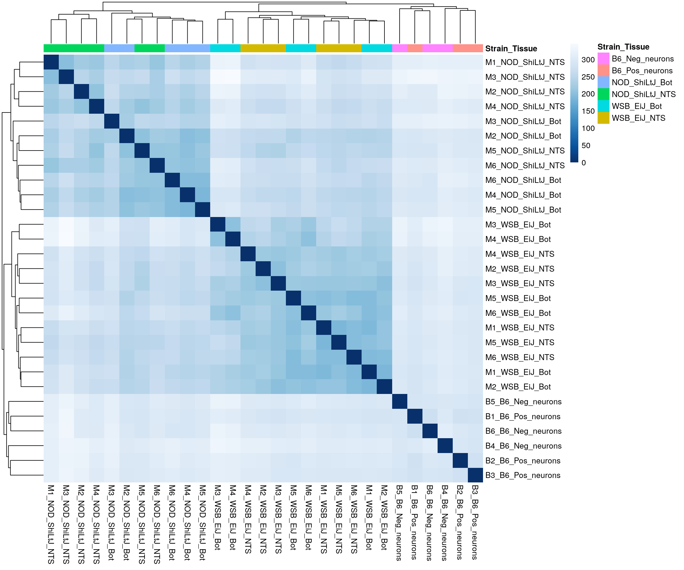
| Version | Author | Date |
|---|---|---|
| 50e8649 | xhyuo | 2022-10-13 |
#heatmap on correlation matrix
rld_cor <- cor(assay(rld))
pheatmap(rld_cor,
         annotation_col  = df,
         clustering_distance_rows = "correlation",
         clustering_distance_cols = "correlation",
         border_color = NA)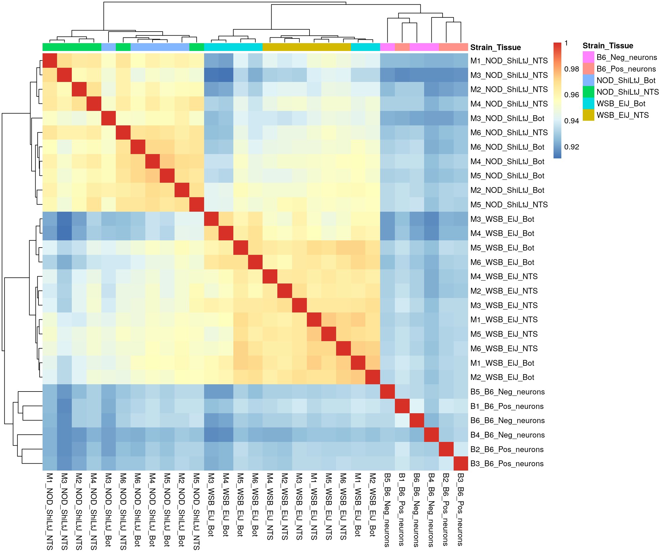
| Version | Author | Date |
|---|---|---|
| 50e8649 | xhyuo | 2022-10-13 |
#PCA plot
#Another way to visualize sample-to-sample distances is a principal components analysis (PCA).
pca.plot <- plotPCA(rld, intgroup = c("Strain_Tissue"), returnData = FALSE)
pca.plot$data$name = ""
pca.plot + geom_text(aes(label=name))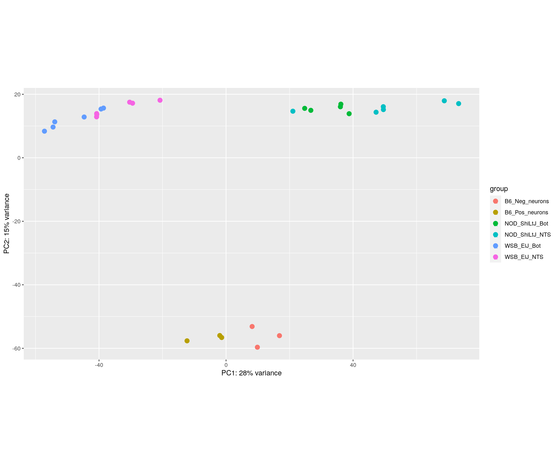
| Version | Author | Date |
|---|---|---|
| 50e8649 | xhyuo | 2022-10-13 |
#subset to NOD-bot and B6
id = rownames(design.matrix[design.matrix$Strain_Tissue %in% c("NOD_ShiLtJ_Bot", "B6_Pos_neurons", "B6_Neg_neurons"),])

#The variance stabilizing transformation and the rlog
#The rlog tends to work well on small datasets (n < 30), potentially outperforming the VST when there is a wide range of sequencing depth across samples (an order of magnitude difference).
#sample distance
sampleDists <- dist(t(assay(rld)[,id]))
sampleDistMatrix <- as.matrix( sampleDists )
colors <- colorRampPalette( rev(brewer.pal(9, "Blues")) )(255)
#annotation
df <- as.data.frame(colData(ddsMat)[id, c("Strain_Tissue")])
colnames(df) = "Strain_Tissue"
rownames(df) = rownames(sampleDistMatrix)

#heatmap on sample distance
pheatmap(sampleDistMatrix,
         clustering_distance_rows = sampleDists,
         clustering_distance_cols = sampleDists,
         col = colors,
         annotation_col  = df,
         border_color = NA)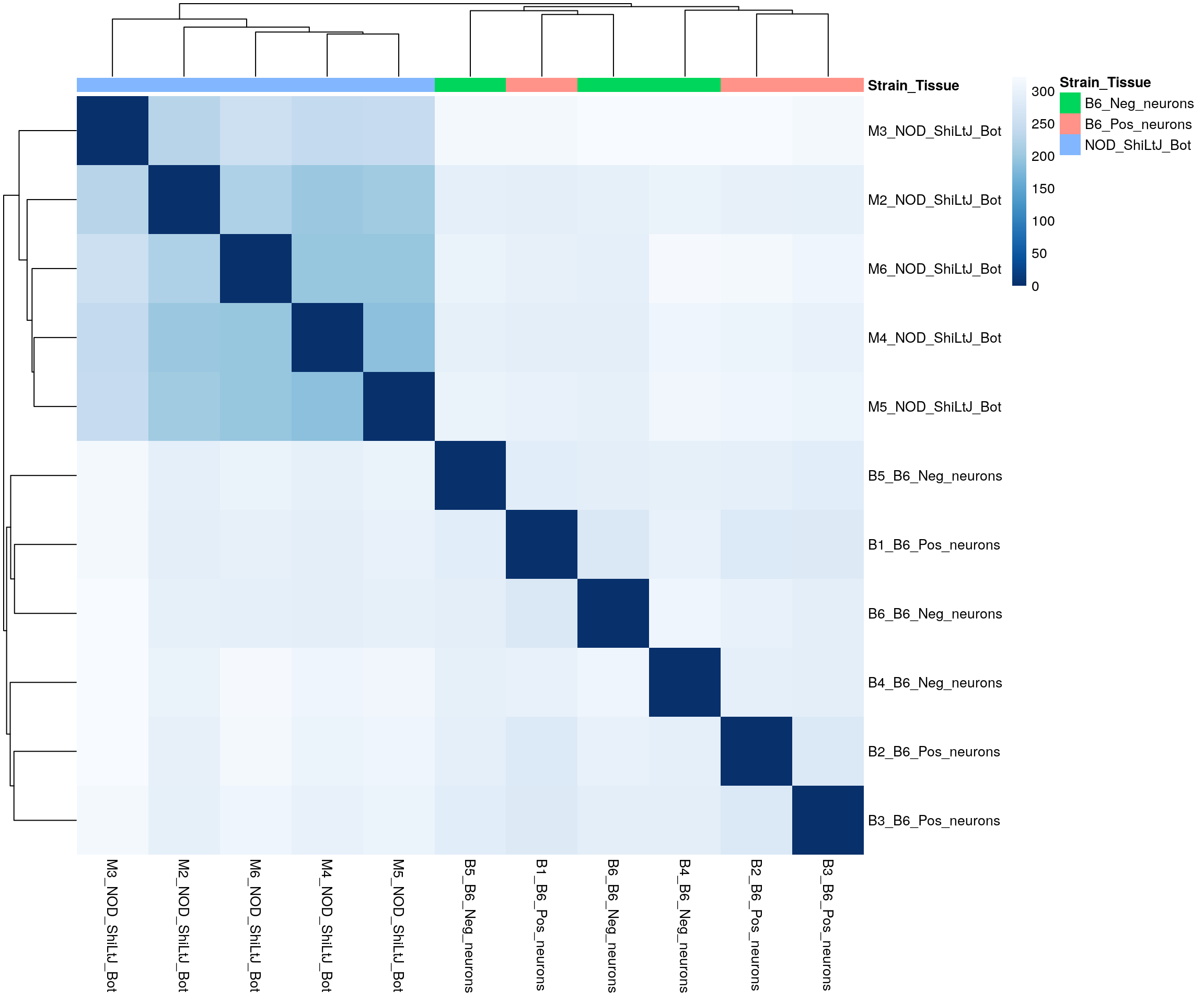
#heatmap on correlation matrix
rld_cor <- cor(assay(rld)[, id])
pheatmap(rld_cor,
         annotation_col  = df,
         clustering_distance_rows = "correlation",
         clustering_distance_cols = "correlation",
         border_color = NA)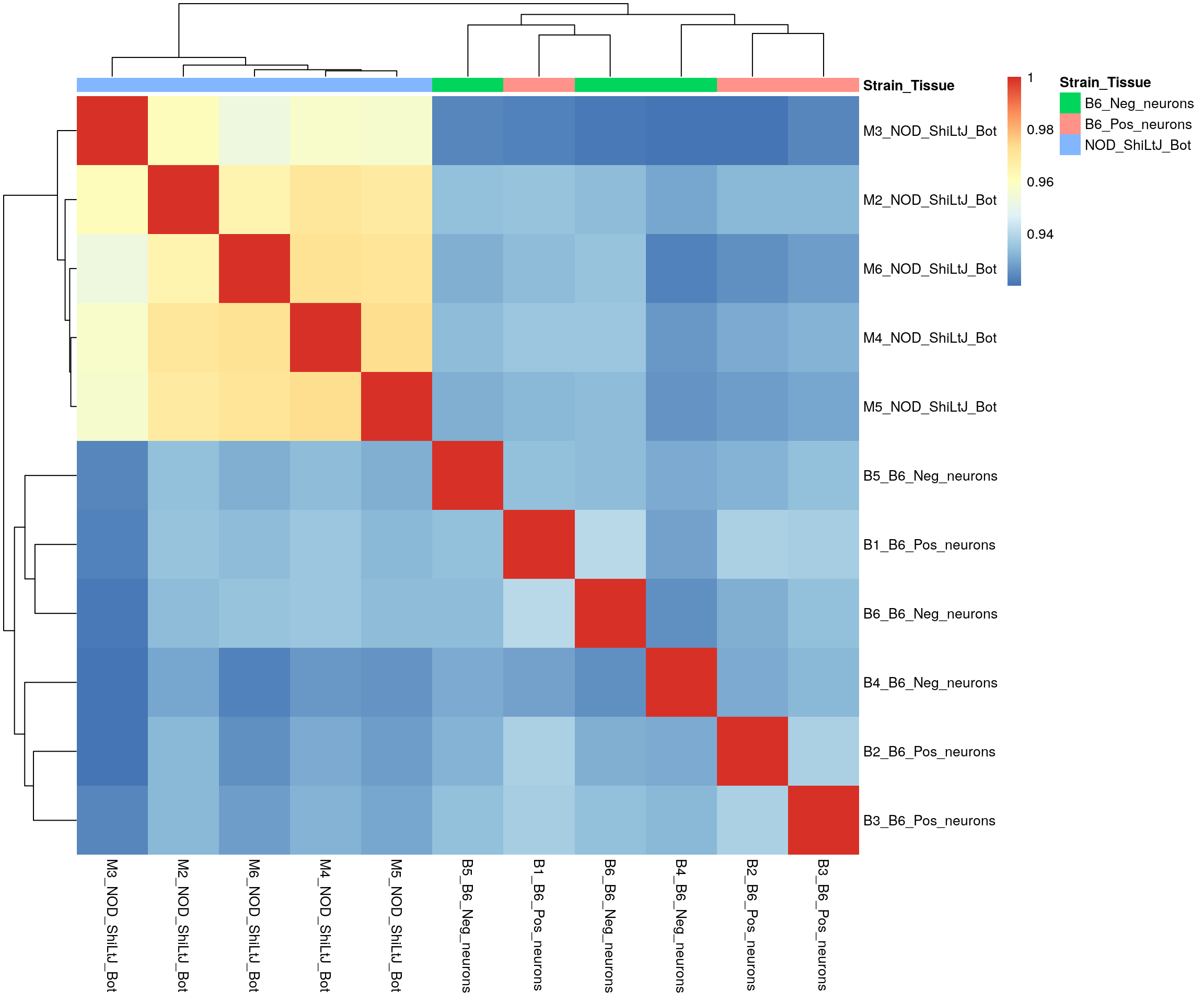
#PCA plot
#Another way to visualize sample-to-sample distances is a principal components analysis (PCA).
pca.plot <- plotPCA(rld[, id], intgroup = c("Strain_Tissue"), returnData = FALSE)
pca.plot$data$name = ""
pca.plot + geom_text(aes(label=name))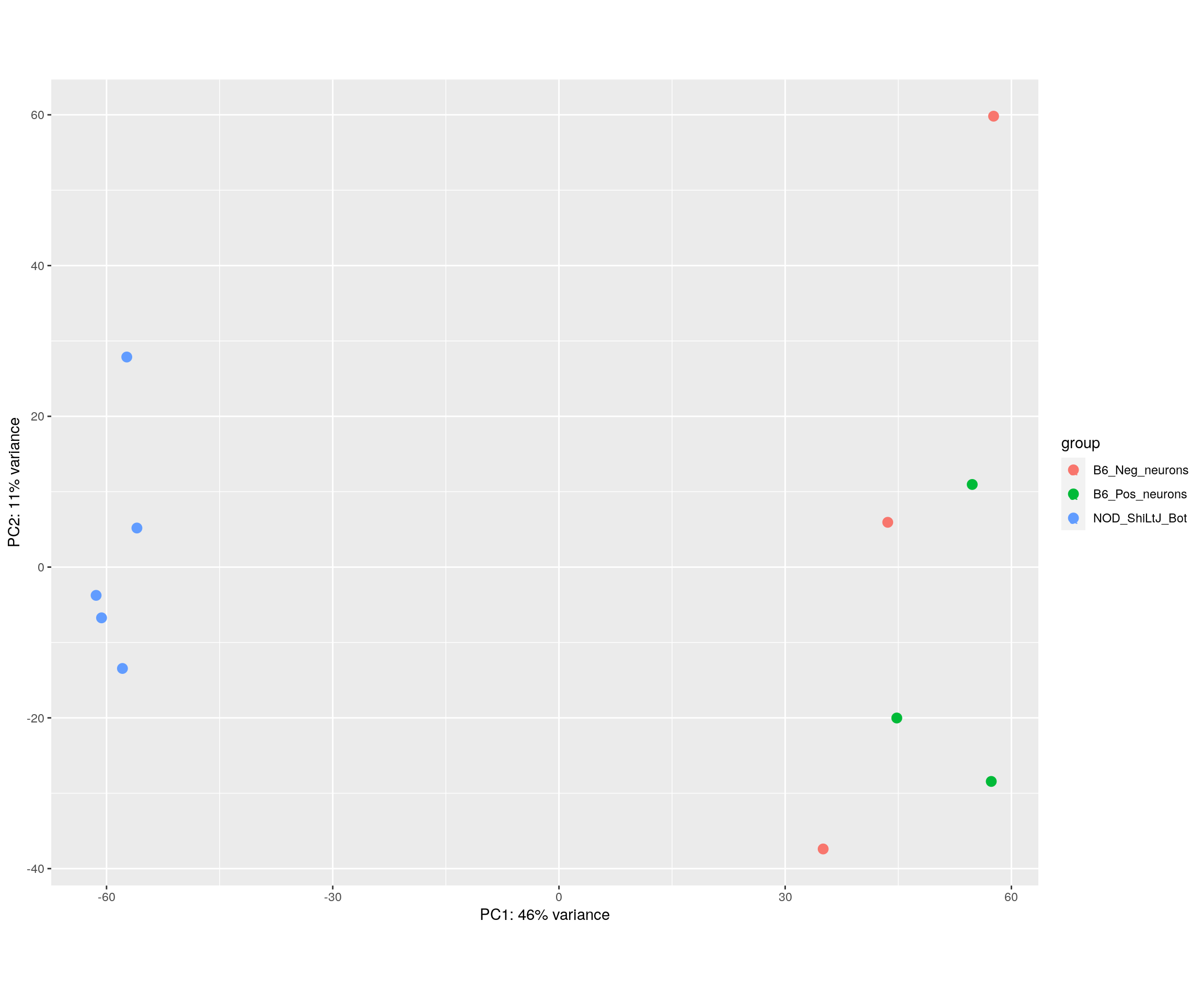
Differential gene expression analysis of Strain_Tissue_NOD_ShiLtJ_Bot_vs_B6_Pos_neurons
design(ddsMat)~Strain_Tissue#Running the differential expression pipeline
res <- DESeq(ddsMat)estimating size factorsestimating dispersionsgene-wise dispersion estimatesmean-dispersion relationshipfinal dispersion estimatesfitting model and testingresultsNames(res)[1] "Intercept"
[2] "Strain_Tissue_B6_Pos_neurons_vs_B6_Neg_neurons"
[3] "Strain_Tissue_NOD_ShiLtJ_Bot_vs_B6_Neg_neurons"
[4] "Strain_Tissue_NOD_ShiLtJ_NTS_vs_B6_Neg_neurons"
[5] "Strain_Tissue_WSB_EiJ_Bot_vs_B6_Neg_neurons"
[6] "Strain_Tissue_WSB_EiJ_NTS_vs_B6_Neg_neurons" #comparison for Strain_Tissue_NOD_ShiLtJ_Bot_vs_B6_Pos_neurons------
fdr = 0.01
#Building the results table
res.tab <- results(res, contrast=c("Strain_Tissue","NOD_ShiLtJ_Bot","B6_Pos_neurons"), alpha = 0.05)
res.tablog2 fold change (MLE): Strain_Tissue NOD_ShiLtJ_Bot vs B6_Pos_neurons
Wald test p-value: Strain_Tissue NOD_ShiLtJ_Bot vs B6_Pos_neurons
DataFrame with 31329 rows and 6 columns
baseMean log2FoldChange lfcSE stat
<numeric> <numeric> <numeric> <numeric>
ENSMUSG00000000001_Gnai3 1006.18087 0.00575975 0.259557 0.0221907
ENSMUSG00000000028_Cdc45 39.89799 -0.83405015 1.175907 -0.7092825
ENSMUSG00000000031_H19 27.36166 -0.91677621 1.023646 -0.8955989
ENSMUSG00000000037_Scml2 40.35147 -0.28270786 0.717862 -0.3938194
ENSMUSG00000000049_Apoh 5.54456 -0.19593863 1.256068 -0.1559937
... ... ... ... ...
ENSMUSG00000118643_AC163703.1 2.03021 -2.705450 2.98313 -0.906916
ENSMUSG00000118646_AC160405.1 3.36031 2.172474 1.64977 1.316831
ENSMUSG00000118651_CT030740.1 11.51722 0.860985 1.01691 0.846670
ENSMUSG00000118653_AC159819.1 2.69970 -5.831060 3.40583 -1.712084
ENSMUSG00000118655_AC156032.1 6.63847 -7.960012 3.97281 -2.003625
pvalue padj
<numeric> <numeric>
ENSMUSG00000000001_Gnai3 0.982296 0.999349
ENSMUSG00000000028_Cdc45 0.478149 0.797325
ENSMUSG00000000031_H19 0.370467 0.726655
ENSMUSG00000000037_Scml2 0.693714 0.900761
ENSMUSG00000000049_Apoh 0.876038 0.968355
... ... ...
ENSMUSG00000118643_AC163703.1 0.3644515 0.722637
ENSMUSG00000118646_AC160405.1 0.1878954 0.551873
ENSMUSG00000118651_CT030740.1 0.3971789 0.745857
ENSMUSG00000118653_AC159819.1 0.0868812 0.376273
ENSMUSG00000118655_AC156032.1 0.0451102 0.257488summary(res.tab)
out of 31329 with nonzero total read count
adjusted p-value < 0.05
LFC > 0 (up)       : 1419, 4.5%
LFC < 0 (down)     : 765, 2.4%
outliers [1]       : 548, 1.7%
low counts [2]     : 5407, 17%
(mean count < 2)
[1] see 'cooksCutoff' argument of ?results
[2] see 'independentFiltering' argument of ?results
table(res.tab$padj < fdr)
FALSE  TRUE
23981  1393
#We subset the results table to these genes and then sort it by the log2 fold change estimate to get the significant genes with the strongest down-regulation:
resSig <- subset(res.tab, padj < fdr)
head(resSig[order(resSig$log2FoldChange), ])log2 fold change (MLE): Strain_Tissue NOD_ShiLtJ_Bot vs B6_Pos_neurons
Wald test p-value: Strain_Tissue NOD_ShiLtJ_Bot vs B6_Pos_neurons
DataFrame with 6 rows and 6 columns
baseMean log2FoldChange lfcSE stat
<numeric> <numeric> <numeric> <numeric>
ENSMUSG00000066407_Gm10263 38.3327 -27.6567 5.74808 -4.81146
ENSMUSG00000105018_Gm43546 12.9746 -22.7874 5.76286 -3.95419
ENSMUSG00000108774_Gm45136 12.9746 -22.7874 5.76286 -3.95419
ENSMUSG00000045132_Olfr620 5371.4891 -18.1623 3.58579 -5.06507
ENSMUSG00000110252_Gm2961 2090.0918 -16.3126 3.49444 -4.66816
ENSMUSG00000100595_Gm19087 557.8766 -14.9298 3.56203 -4.19138
pvalue padj
<numeric> <numeric>
ENSMUSG00000066407_Gm10263 1.49830e-06 7.15967e-05
ENSMUSG00000105018_Gm43546 7.67938e-05 2.07816e-03
ENSMUSG00000108774_Gm45136 7.67938e-05 2.07816e-03
ENSMUSG00000045132_Olfr620 4.08260e-07 2.28679e-05
ENSMUSG00000110252_Gm2961 3.03908e-06 1.32497e-04
ENSMUSG00000100595_Gm19087 2.77268e-05 8.96228e-04# with the strongest up-regulation:
head(resSig[order(resSig$log2FoldChange, decreasing = TRUE), ])log2 fold change (MLE): Strain_Tissue NOD_ShiLtJ_Bot vs B6_Pos_neurons
Wald test p-value: Strain_Tissue NOD_ShiLtJ_Bot vs B6_Pos_neurons
DataFrame with 6 rows and 6 columns
baseMean log2FoldChange lfcSE stat
<numeric> <numeric> <numeric> <numeric>
ENSMUSG00000094248_Hist1h2ao 28.9568 40.8362 5.37374 7.59922
ENSMUSG00000112012_Gm47025 100.9697 37.2580 2.32883 15.99858
ENSMUSG00000035539_Ccdc180 29.2975 36.8045 2.02150 18.20653
ENSMUSG00000078087_Rps12l1 19.4819 36.7635 5.79521 6.34378
ENSMUSG00000084010_Gm13302 152.1574 36.0407 3.01201 11.96565
ENSMUSG00000105340_Gm42878 16.9882 34.4038 5.79839 5.93333
pvalue padj
<numeric> <numeric>
ENSMUSG00000094248_Hist1h2ao 2.97925e-14 5.55848e-12
ENSMUSG00000112012_Gm47025 1.30716e-57 1.65839e-53
ENSMUSG00000035539_Ccdc180 4.58076e-74 1.16232e-69
ENSMUSG00000078087_Rps12l1 2.24198e-10 2.63371e-08
ENSMUSG00000084010_Gm13302 5.37775e-33 1.04965e-29
ENSMUSG00000105340_Gm42878 2.96858e-09 2.58848e-07#Visualization---------------------
#Volcano plot
## Obtain logical vector regarding whether padj values are less than 0.05
threshold_OE <- (res.tab$padj < fdr & abs(res.tab$log2FoldChange) >= 1)
## Determine the number of TRUE values
length(which(threshold_OE))[1] 1321## Add logical vector as a column (threshold) to the res.tab
res.tab$threshold <- threshold_OE
## Sort by ordered padj
res.tab_ordered <- res.tab %>%
data.frame() %>%
rownames_to_column(var="ENSEMBL") %>%
tidyr::separate(., ENSEMBL, c("ENSEMBL", "SYMBOL"), sep = "_") %>%
arrange(padj) %>%
mutate(genelabels = "") %>%
as_tibble()
## Create a column to indicate which genes to label
res.tab_ordered$genelabels[1:10] <- res.tab_ordered$SYMBOL[1:10]
#display res.tab_ordered
DT::datatable(res.tab_ordered[res.tab_ordered$padj < fdr,],
filter = list(position = 'top', clear = FALSE),
extensions = 'Buttons',
options = list(dom = 'Blfrtip',
buttons = c('csv', 'excel'),
lengthMenu = list(c(10,25,50,-1),
c(10,25,50,"All")),
pageLength = 40,
scrollY = "300px",
scrollX = "40px"),
caption = htmltools::tags$caption(style = 'caption-side: top; text-align: left; color:black; font-size:200% ;','DEG for NOD_ShiLtJ_Bot_vs_B6_Pos_neurons (fdr < 0.01)'))#Volcano plot
volcano.plot <- ggplot(res.tab_ordered) +
geom_point(aes(x = log2FoldChange, y = -log10(padj), colour = threshold)) +
scale_color_manual(values=c("blue", "red")) +
geom_text_repel(aes(x = log2FoldChange, y = -log10(padj),
label = genelabels,
size = 3.5)) +
ggtitle("DEG for NOD_ShiLtJ_Bot_vs_B6_Pos_neurons") +
xlab("log2 fold change") +
ylab("-log10 adjusted p-value") +
theme(legend.position = "none",
plot.title = element_text(size = rel(1.5), hjust = 0.5),
axis.title = element_text(size = rel(1.25)))
print(volcano.plot)Warning: Removed 5955 rows containing missing values (geom_point).Warning: Removed 5955 rows containing missing values (geom_text_repel).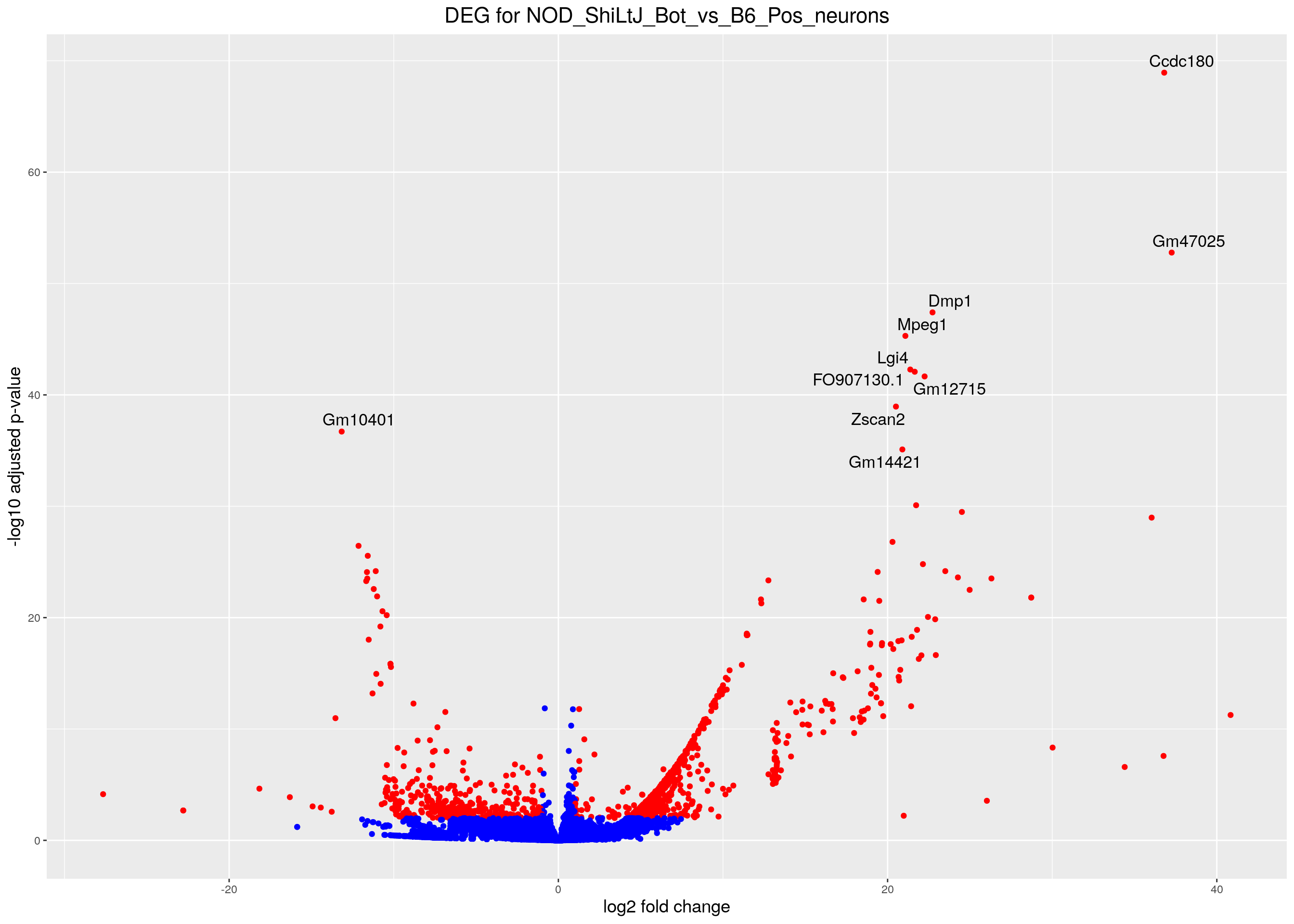
| Version | Author | Date |
|---|---|---|
| 50e8649 | xhyuo | 2022-10-13 |
#heatmap
# Extract normalized expression for significant genes fdr < 0.000001 & abs(log2FoldChange) >= 1)
normalized_counts_sig <- normalized_counts %>%
  filter(gene %in% rownames(subset(resSig, padj < 0.000001 & abs(log2FoldChange) >= 1)))
#Set a color palette
heat_colors <- brewer.pal(6, "YlOrRd")
#Run pheatmap using the metadata data frame for the annotation
pheatmap(as.matrix(normalized_counts_sig[,-1]),
         color = heat_colors,
         cluster_rows = T,
         show_rownames = F,
         annotation_col  = df,
         border_color = NA,
         fontsize = 10,
         scale = "row",
         fontsize_row = 10,
         height = 20,
         main = "Heatmap of the top DEGs in NOD_ShiLtJ_Bot_vs_B6_Pos_neurons (fdr < 0.000001 & abs(log2FoldChange) >= 1)")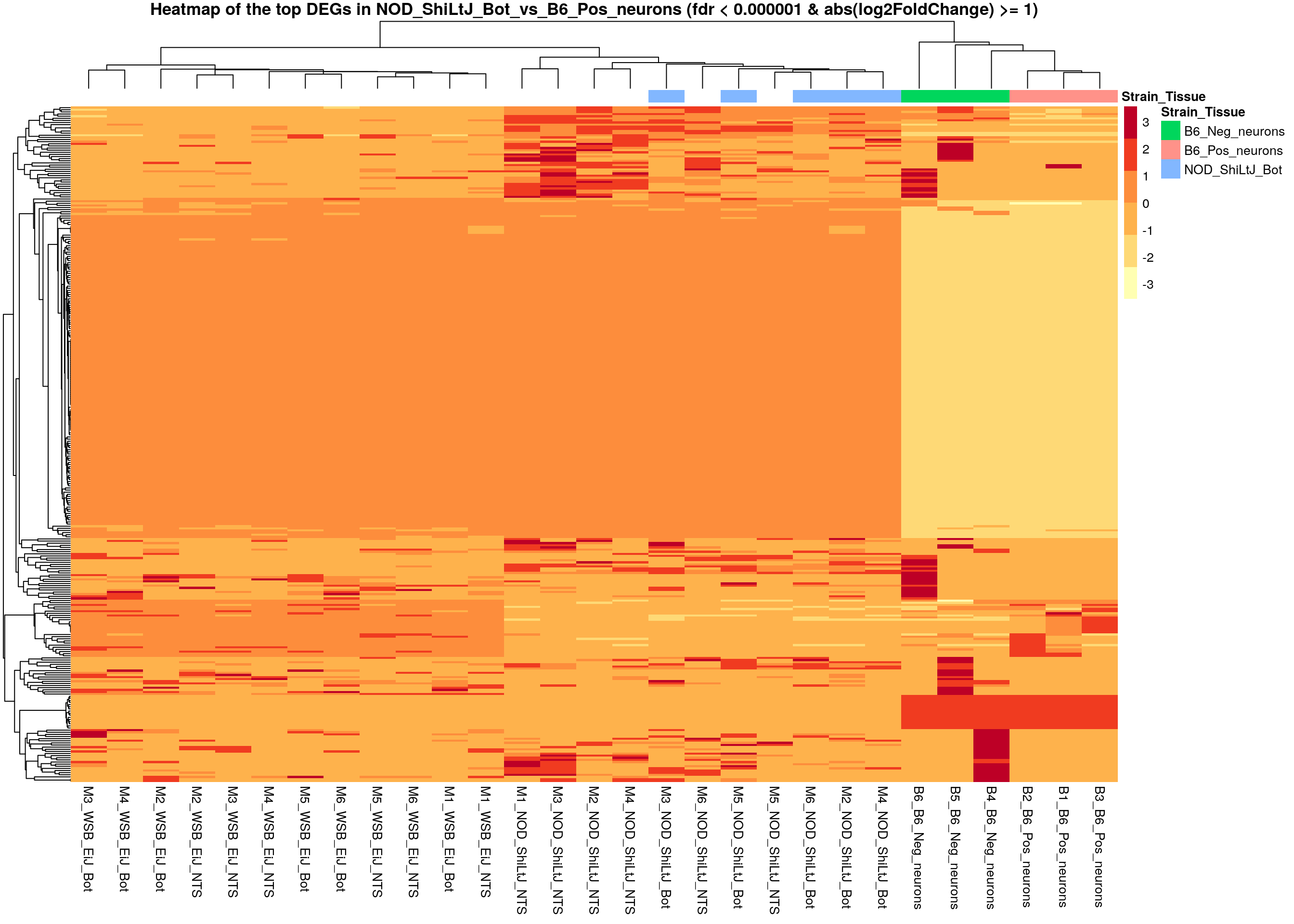
| Version | Author | Date |
|---|---|---|
| 50e8649 | xhyuo | 2022-10-13 |
#Enrichment----------------------
#enrichment analysis
dbs <- c("WikiPathways_2019_Mouse",
         "GO_Biological_Process_2021",
         "GO_Cellular_Component_2021",
         "GO_Molecular_Function_2021",
         "KEGG_2019_Mouse",
         "Mouse_Gene_Atlas",
         "MGI_Mammalian_Phenotype_Level_4_2019")

#results------
resSig.tab <- resSig %>%
  data.frame() %>%
  rownames_to_column(var="ENSEMBL") %>%
  as_tibble() %>%
  tidyr::separate(., ENSEMBL, c("ENSEMBL", "SYMBOL"), sep = "_")

#up-regulated tissue genes---------------------------
up.genes <- resSig.tab %>%
  filter(log2FoldChange > 0) %>%
  pull(SYMBOL)
#up-regulated genes enrichment
up.genes.enriched <- enrichr(as.character(na.omit(up.genes)), dbs)
Uploading data to Enrichr... Done.
Querying WikiPathways_2019_Mouse... Done.
Querying GO_Biological_Process_2021... Done.
Querying GO_Cellular_Component_2021... Done.
Querying GO_Molecular_Function_2021... Done.
Querying KEGG_2019_Mouse... Done.
Querying Mouse_Gene_Atlas... Done.
Querying MGI_Mammalian_Phenotype_Level_4_2019... Done.
Parsing results... Done.for (j in 1:length(up.genes.enriched)){
up.genes.enriched[[j]] <- cbind(data.frame(Library = names(up.genes.enriched)[j]),up.genes.enriched[[j]])
}
up.genes.enriched <- do.call(rbind.data.frame, up.genes.enriched) %>%
filter(Adjusted.P.value <= 0.1) %>%
mutate(logpvalue = -log10(P.value)) %>%
arrange(desc(logpvalue)) %>%
tibble::remove_rownames()
#display up.genes.enriched
DT::datatable(up.genes.enriched,filter = list(position = 'top', clear = FALSE),
options = list(pageLength = 40, scrollY = "300px", scrollX = "40px"))#barpot
up.genes.enriched.plot <- up.genes.enriched %>%
filter(Adjusted.P.value <= 0.1) %>%
mutate(Term = fct_reorder(Term, -logpvalue)) %>%
ggplot(data = ., aes(x = Term, y = logpvalue, fill = Library, label = Overlap)) +
geom_bar(stat = "identity") +
geom_text(position = position_dodge(width = 0.9),
hjust = 0) +
theme_bw() +
ylab("-log(p.value)") +
xlab("") +
ggtitle("Enrichment of up-regulated tissue genes \n(Adjusted.P.value <= 0.1)") +
theme(plot.background = element_blank() ,
panel.border = element_blank(),
panel.background = element_blank(),
#legend.position = "none",
plot.title = element_text(hjust = 0),
panel.grid.major = element_blank(),
panel.grid.minor = element_blank()) +
theme(axis.line = element_line(color = 'black')) +
theme(axis.title.x = element_text(size = 12, vjust=-0.5)) +
theme(axis.title.y = element_text(size = 12, vjust= 1.0)) +
theme(axis.text = element_text(size = 12)) +
theme(plot.title = element_text(size = 12)) +
coord_flip()
up.genes.enriched.plot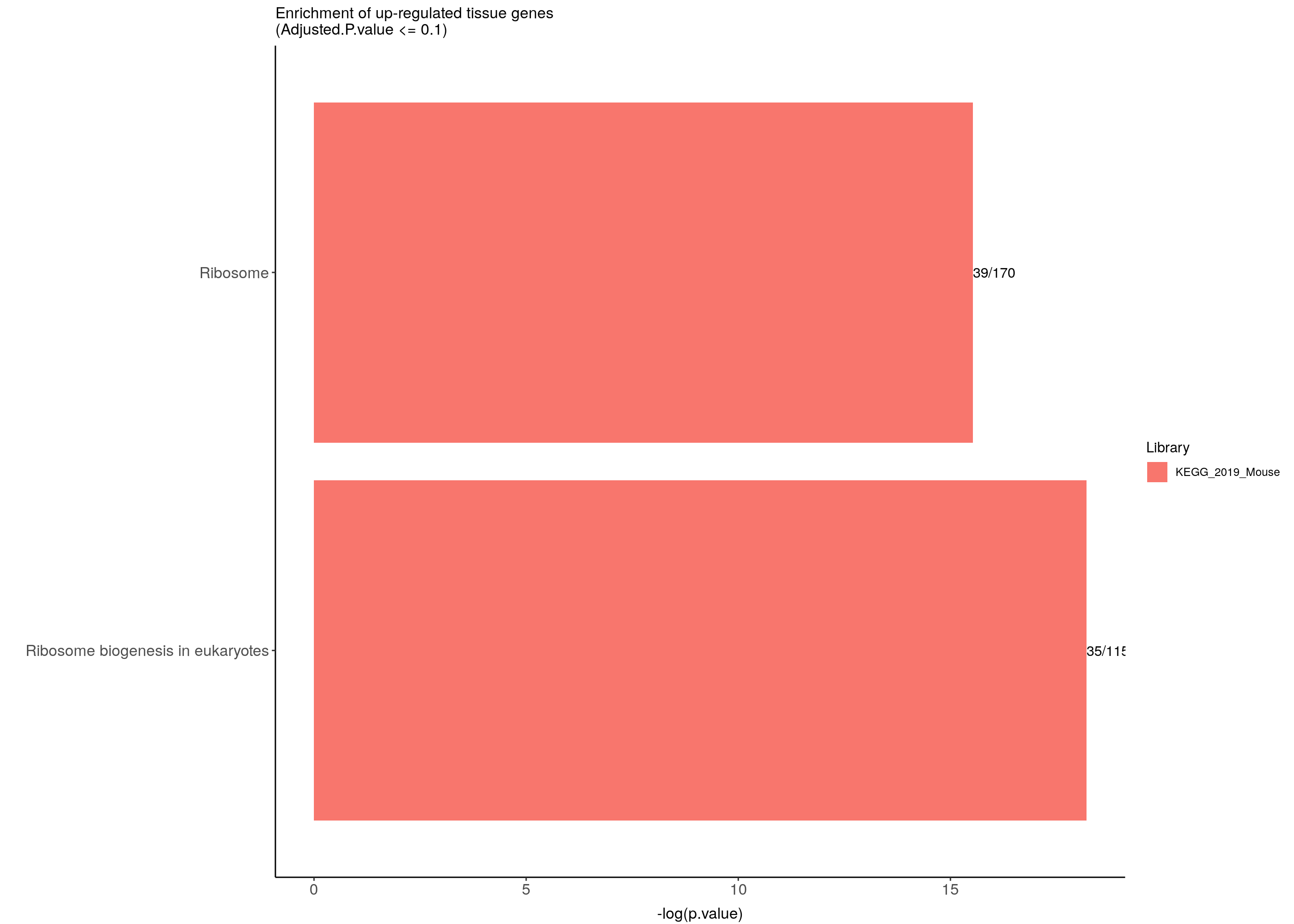
| Version | Author | Date |
|---|---|---|
| 50e8649 | xhyuo | 2022-10-13 |
#down-regulated tissue genes---------------------------
down.genes <- resSig.tab %>%
  filter(log2FoldChange < 0) %>%
  pull(SYMBOL)
#down-regulated genes enrichment
down.genes.enriched <- enrichr(as.character(na.omit(down.genes)), dbs)
Uploading data to Enrichr... Done.
Querying WikiPathways_2019_Mouse... Done.
Querying GO_Biological_Process_2021... Done.
Querying GO_Cellular_Component_2021... Done.
Querying GO_Molecular_Function_2021... Done.
Querying KEGG_2019_Mouse... Done.
Querying Mouse_Gene_Atlas... Done.
Querying MGI_Mammalian_Phenotype_Level_4_2019... Done.
Parsing results... Done.for (j in 1:length(down.genes.enriched)){
down.genes.enriched[[j]] <- cbind(data.frame(Library = names(down.genes.enriched)[j]),down.genes.enriched[[j]])
}
down.genes.enriched <- do.call(rbind.data.frame, down.genes.enriched) %>%
filter(Adjusted.P.value <= 0.35) %>%
mutate(logpvalue = -log10(P.value)) %>%
arrange(desc(logpvalue)) %>%
tibble::remove_rownames()
#display down.genes.enriched
DT::datatable(down.genes.enriched,filter = list(position = 'top', clear = FALSE),
options = list(pageLength = 40, scrollY = "300px", scrollX = "40px"))#barpot
down.genes.enriched.plot <- down.genes.enriched %>%
filter(Adjusted.P.value <= 0.35) %>%
mutate(Term = fct_reorder(Term, -logpvalue)) %>%
ggplot(data = ., aes(x = Term, y = logpvalue, fill = Library, label = Overlap)) +
geom_bar(stat = "identity") +
geom_text(position = position_dodge(width = 0.9),
hjust = 0) +
theme_bw() +
ylab("-log(p.value)") +
xlab("") +
ggtitle("Enrichment of down-regulated tissue genes \n(Adjusted.P.value <= 0.35)") +
theme(plot.background = element_blank() ,
panel.border = element_blank(),
panel.background = element_blank(),
#legend.position = "none",
plot.title = element_text(hjust = 0),
panel.grid.major = element_blank(),
panel.grid.minor = element_blank()) +
theme(axis.line = element_line(color = 'black')) +
theme(axis.title.x = element_text(size = 12, vjust=-0.5)) +
theme(axis.title.y = element_text(size = 12, vjust= 1.0)) +
theme(axis.text = element_text(size = 12)) +
theme(plot.title = element_text(size = 12)) +
coord_flip()
down.genes.enriched.plot
| Version | Author | Date |
|---|---|---|
| 50e8649 | xhyuo | 2022-10-13 |
Differential gene expression analysis of Strain_Tissue_NOD_ShiLtJ_Bot_vs_B6_Neg_neurons
#comparison for Strain_Tissue_NOD_ShiLtJ_Bot_vs_B6_Neg_neurons------
fdr = 0.01
#Building the results table
res.tab <- results(res, contrast=c("Strain_Tissue","NOD_ShiLtJ_Bot","B6_Neg_neurons"), alpha = 0.05)
res.tab
log2 fold change (MLE): Strain_Tissue NOD_ShiLtJ_Bot vs B6_Neg_neurons
Wald test p-value: Strain Tissue NOD ShiLtJ Bot vs B6 Neg neurons
DataFrame with 31329 rows and 6 columns
baseMean log2FoldChange lfcSE stat
<numeric> <numeric> <numeric> <numeric>
ENSMUSG00000000001_Gnai3 1006.18087 0.2524407 0.260507 0.9690381
ENSMUSG00000000028_Cdc45 39.89799 -0.5336417 1.182218 -0.4513901
ENSMUSG00000000031_H19 27.36166 -1.4325922 0.995003 -1.4397866
ENSMUSG00000000037_Scml2 40.35147 -0.3871429 0.709509 -0.5456487
ENSMUSG00000000049_Apoh 5.54456 -0.0671984 1.264671 -0.0531351
... ... ... ... ...
ENSMUSG00000118643_AC163703.1 2.03021 -3.083175 2.951339 -1.044670
ENSMUSG00000118646_AC160405.1 3.36031 2.256177 1.649759 1.367580
ENSMUSG00000118651_CT030740.1 11.51722 -0.379417 0.850877 -0.445913
ENSMUSG00000118653_AC159819.1 2.69970 -6.513683 3.363715 -1.936455
ENSMUSG00000118655_AC156032.1 6.63847 -8.417454 3.966468 -2.122153
pvalue padj
<numeric> <numeric>
ENSMUSG00000000001_Gnai3 0.332526 0.728360
ENSMUSG00000000028_Cdc45 0.651708 0.903834
ENSMUSG00000000031_H19 0.149928 0.518781
ENSMUSG00000000037_Scml2 0.585307 0.879624
ENSMUSG00000000049_Apoh 0.957624 0.993287
... ... ...
ENSMUSG00000118643_AC163703.1 0.2961756 NA
ENSMUSG00000118646_AC160405.1 0.1714436 0.548297
ENSMUSG00000118651_CT030740.1 0.6556604 0.904553
ENSMUSG00000118653_AC159819.1 0.0528120 0.293105
ENSMUSG00000118655_AC156032.1 0.0338249 0.222135summary(res.tab)
out of 31329 with nonzero total read count
adjusted p-value < 0.05
LFC > 0 (up)       : 1394, 4.4%
LFC < 0 (down)     : 669, 2.1%
outliers [1]       : 548, 1.7%
low counts [2]     : 5999, 19%
(mean count < 2)
[1] see 'cooksCutoff' argument of ?results
[2] see 'independentFiltering' argument of ?results
table(res.tab$padj < fdr)
FALSE  TRUE
23430  1352
#We subset the results table to these genes and then sort it by the log2 fold change estimate to get the significant genes with the strongest down-regulation:
resSig <- subset(res.tab, padj < fdr)
head(resSig[order(resSig$log2FoldChange), ])log2 fold change (MLE): Strain_Tissue NOD_ShiLtJ_Bot vs B6_Neg_neurons
Wald test p-value: Strain Tissue NOD ShiLtJ Bot vs B6 Neg neurons
DataFrame with 6 rows and 6 columns
baseMean log2FoldChange lfcSE stat
<numeric> <numeric> <numeric> <numeric>
ENSMUSG00000066407_Gm10263 38.3327 -26.6035 5.74907 -4.62744
ENSMUSG00000105018_Gm43546 12.9746 -21.9633 5.77339 -3.80424
ENSMUSG00000108774_Gm45136 12.9746 -21.9633 5.77339 -3.80424
ENSMUSG00000045132_Olfr620 5371.4891 -17.4986 3.58570 -4.88012
ENSMUSG00000110252_Gm2961 2090.0918 -16.6773 3.49433 -4.77267
ENSMUSG00000100595_Gm19087 557.8766 -14.1745 3.56204 -3.97933
pvalue padj
<numeric> <numeric>
ENSMUSG00000066407_Gm10263 3.70210e-06 0.000161524
ENSMUSG00000105018_Gm43546 1.42242e-04 0.003396802
ENSMUSG00000108774_Gm45136 1.42242e-04 0.003396802
ENSMUSG00000045132_Olfr620 1.06022e-06 0.000055666
ENSMUSG00000110252_Gm2961 1.81801e-06 0.000088168
ENSMUSG00000100595_Gm19087 6.91090e-05 0.001915114# with the strongest up-regulation:
head(resSig[order(resSig$log2FoldChange, decreasing = TRUE), ])log2 fold change (MLE): Strain_Tissue NOD_ShiLtJ_Bot vs B6_Neg_neurons
Wald test p-value: Strain Tissue NOD ShiLtJ Bot vs B6 Neg neurons
DataFrame with 6 rows and 6 columns
baseMean log2FoldChange lfcSE stat
<numeric> <numeric> <numeric> <numeric>
ENSMUSG00000005716_Pvalb 886.203 22.7762 2.44280 9.32382
ENSMUSG00000037280_Galnt6 394.304 21.1380 1.48946 14.19174
ENSMUSG00000036964_Trim17 105.565 20.3731 2.27823 8.94250
ENSMUSG00000068397_Gm10240 196.588 20.3252 2.75583 7.37533
ENSMUSG00000084383_Gm13370 196.588 20.3252 2.75583 7.37533
ENSMUSG00000091712_Sec14l5 650.320 20.2714 2.40342 8.43437
pvalue padj
<numeric> <numeric>
ENSMUSG00000005716_Pvalb 1.12222e-20 7.01280e-18
ENSMUSG00000037280_Galnt6 1.03070e-45 2.55427e-41
ENSMUSG00000036964_Trim17 3.80452e-19 1.97346e-16
ENSMUSG00000068397_Gm10240 1.63935e-13 3.54245e-11
ENSMUSG00000084383_Gm13370 1.63935e-13 3.54245e-11
ENSMUSG00000091712_Sec14l5 3.32987e-17 1.30986e-14#Visualization---------------------
#Volcano plot
## Obtain logical vector regarding whether padj values are less than 0.05
threshold_OE <- (res.tab$padj < fdr & abs(res.tab$log2FoldChange) >= 1)
## Determine the number of TRUE values
length(which(threshold_OE))[1] 1302## Add logical vector as a column (threshold) to the res.tab
res.tab$threshold <- threshold_OE
## Sort by ordered padj
res.tab_ordered <- res.tab %>%
data.frame() %>%
rownames_to_column(var="ENSEMBL") %>%
tidyr::separate(., ENSEMBL, c("ENSEMBL", "SYMBOL"), sep = "_") %>%
arrange(padj) %>%
mutate(genelabels = "") %>%
as_tibble()
## Create a column to indicate which genes to label
res.tab_ordered$genelabels[1:10] <- res.tab_ordered$SYMBOL[1:10]
#display res.tab_ordered
DT::datatable(res.tab_ordered[res.tab_ordered$padj < fdr,],
filter = list(position = 'top', clear = FALSE),
extensions = 'Buttons',
options = list(dom = 'Blfrtip',
buttons = c('csv', 'excel'),
lengthMenu = list(c(10,25,50,-1),
c(10,25,50,"All")),
pageLength = 40,
scrollY = "300px",
scrollX = "40px"),
caption = htmltools::tags$caption(style = 'caption-side: top; text-align: left; color:black; font-size:200% ;','DEG for NOD_ShiLtJ_Bot_vs_B6_Neg_neurons (fdr < 0.01)'))#Volcano plot
volcano.plot <- ggplot(res.tab_ordered) +
geom_point(aes(x = log2FoldChange, y = -log10(padj), colour = threshold)) +
scale_color_manual(values=c("blue", "red")) +
geom_text_repel(aes(x = log2FoldChange, y = -log10(padj),
label = genelabels,
size = 3.5)) +
ggtitle("DEG for NOD_ShiLtJ_Bot_vs_B6_Neg_neurons") +
xlab("log2 fold change") +
ylab("-log10 adjusted p-value") +
theme(legend.position = "none",
plot.title = element_text(size = rel(1.5), hjust = 0.5),
axis.title = element_text(size = rel(1.25)))
print(volcano.plot)Warning: Removed 6547 rows containing missing values (geom_point).Warning: Removed 6547 rows containing missing values (geom_text_repel).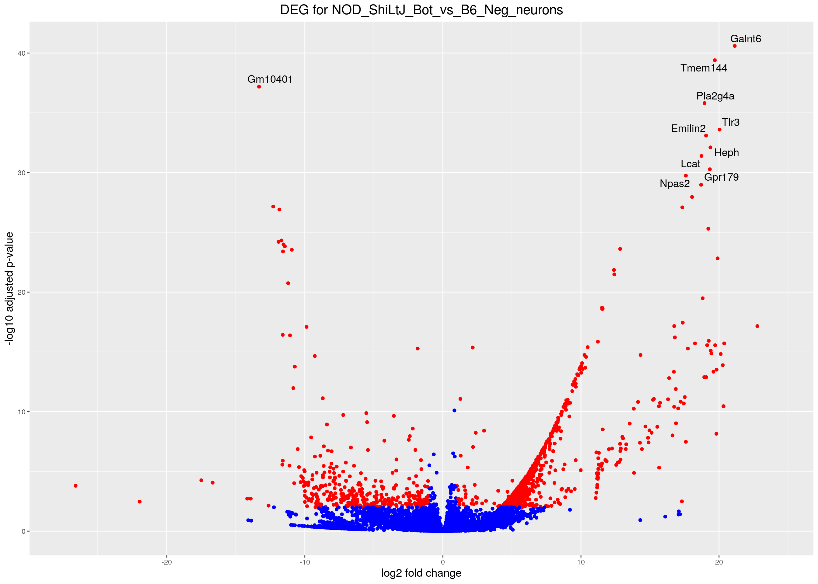
| Version | Author | Date |
|---|---|---|
| 50e8649 | xhyuo | 2022-10-13 |
#heatmap
# Extract normalized expression for significant genes fdr < 0.000001 & abs(log2FoldChange) >= 1)
normalized_counts_sig <- normalized_counts %>%
  filter(gene %in% rownames(subset(resSig, padj < 0.000001 & abs(log2FoldChange) >= 1)))
#Set a color palette
heat_colors <- brewer.pal(6, "YlOrRd")
#Run pheatmap using the metadata data frame for the annotation
pheatmap(as.matrix(normalized_counts_sig[,-1]),
         color = heat_colors,
         cluster_rows = T,
         show_rownames = F,
         annotation_col  = df,
         border_color = NA,
         fontsize = 10,
         scale = "row",
         fontsize_row = 10,
         height = 20,
         main = "Heatmap of the top DEGs in NOD_ShiLtJ_Bot_vs_B6_Neg_neurons (fdr < 0.000001 & abs(log2FoldChange) >= 1)")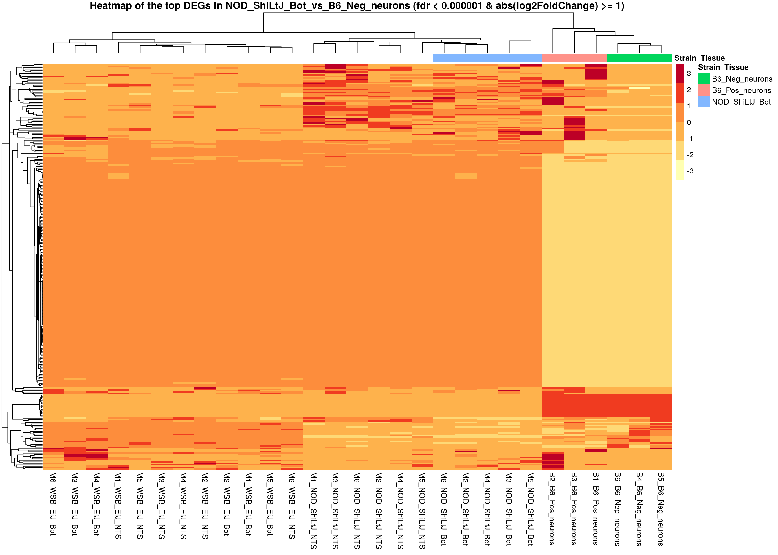
| Version | Author | Date |
|---|---|---|
| 50e8649 | xhyuo | 2022-10-13 |
#Enrichment----------------------
#enrichment analysis
dbs <- c("WikiPathways_2019_Mouse",
         "GO_Biological_Process_2021",
         "GO_Cellular_Component_2021",
         "GO_Molecular_Function_2021",
         "KEGG_2019_Mouse",
         "Mouse_Gene_Atlas",
         "MGI_Mammalian_Phenotype_Level_4_2019")

#results------
resSig.tab <- resSig %>%
  data.frame() %>%
  rownames_to_column(var="ENSEMBL") %>%
  as_tibble() %>%
  tidyr::separate(., ENSEMBL, c("ENSEMBL", "SYMBOL"), sep = "_")

#up-regulated tissue genes---------------------------
up.genes <- resSig.tab %>%
  filter(log2FoldChange > 0) %>%
  pull(SYMBOL)
#up-regulated genes enrichment
up.genes.enriched <- enrichr(as.character(na.omit(up.genes)), dbs)
Uploading data to Enrichr... Done.
Querying WikiPathways_2019_Mouse... Done.
Querying GO_Biological_Process_2021... Done.
Querying GO_Cellular_Component_2021... Done.
Querying GO_Molecular_Function_2021... Done.
Querying KEGG_2019_Mouse... Done.
Querying Mouse_Gene_Atlas... Done.
Querying MGI_Mammalian_Phenotype_Level_4_2019... Done.
Parsing results... Done.for (j in 1:length(up.genes.enriched)){
up.genes.enriched[[j]] <- cbind(data.frame(Library = names(up.genes.enriched)[j]),up.genes.enriched[[j]])
}
up.genes.enriched <- do.call(rbind.data.frame, up.genes.enriched) %>%
filter(Adjusted.P.value <= 0.1) %>%
mutate(logpvalue = -log10(P.value)) %>%
arrange(desc(logpvalue)) %>%
tibble::remove_rownames()
#display up.genes.enriched
DT::datatable(up.genes.enriched,filter = list(position = 'top', clear = FALSE),
options = list(pageLength = 40, scrollY = "300px", scrollX = "40px"))#barpot
up.genes.enriched.plot <- up.genes.enriched %>%
filter(Adjusted.P.value <= 0.1) %>%
mutate(Term = fct_reorder(Term, -logpvalue)) %>%
ggplot(data = ., aes(x = Term, y = logpvalue, fill = Library, label = Overlap)) +
geom_bar(stat = "identity") +
geom_text(position = position_dodge(width = 0.9),
hjust = 0) +
theme_bw() +
ylab("-log(p.value)") +
xlab("") +
ggtitle("Enrichment of up-regulated tissue genes \n(Adjusted.P.value <= 0.1)") +
theme(plot.background = element_blank() ,
panel.border = element_blank(),
panel.background = element_blank(),
#legend.position = "none",
plot.title = element_text(hjust = 0),
panel.grid.major = element_blank(),
panel.grid.minor = element_blank()) +
theme(axis.line = element_line(color = 'black')) +
theme(axis.title.x = element_text(size = 12, vjust=-0.5)) +
theme(axis.title.y = element_text(size = 12, vjust= 1.0)) +
theme(axis.text = element_text(size = 12)) +
theme(plot.title = element_text(size = 12)) +
coord_flip()
up.genes.enriched.plot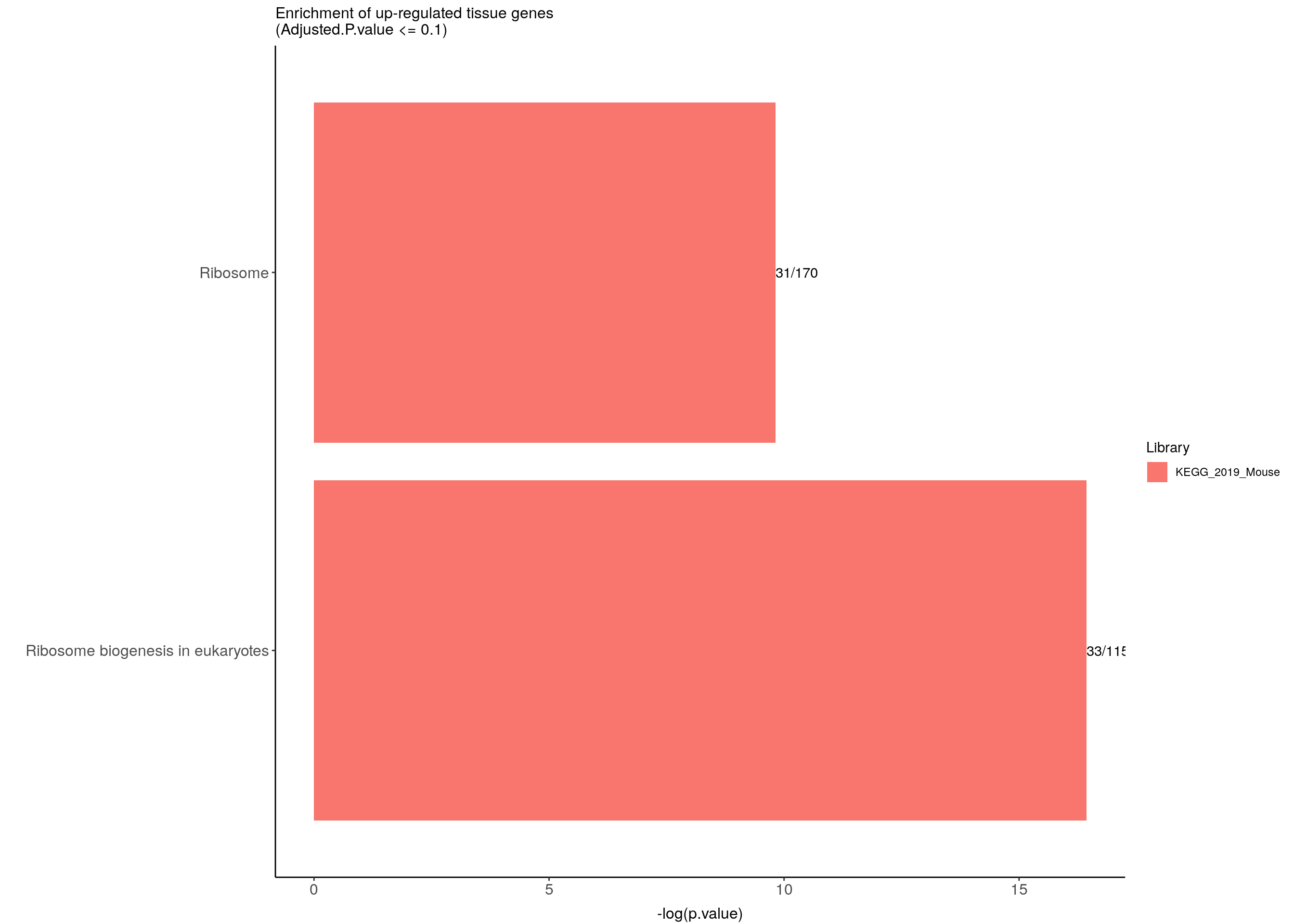
| Version | Author | Date |
|---|---|---|
| 50e8649 | xhyuo | 2022-10-13 |
#down-regulated tissue genes---------------------------
down.genes <- resSig.tab %>%
  filter(log2FoldChange < 0) %>%
  pull(SYMBOL)
#down-regulated genes enrichment
down.genes.enriched <- enrichr(as.character(na.omit(down.genes)), dbs)
Uploading data to Enrichr... Done.
Querying WikiPathways_2019_Mouse... Done.
Querying GO_Biological_Process_2021... Done.
Querying GO_Cellular_Component_2021... Done.
Querying GO_Molecular_Function_2021... Done.
Querying KEGG_2019_Mouse... Done.
Querying Mouse_Gene_Atlas... Done.
Querying MGI_Mammalian_Phenotype_Level_4_2019... Done.
Parsing results... Done.for (j in 1:length(down.genes.enriched)){
down.genes.enriched[[j]] <- cbind(data.frame(Library = names(down.genes.enriched)[j]),down.genes.enriched[[j]])
}
down.genes.enriched <- do.call(rbind.data.frame, down.genes.enriched) %>%
filter(Adjusted.P.value <= 0.5) %>%
mutate(logpvalue = -log10(P.value)) %>%
arrange(desc(logpvalue)) %>%
tibble::remove_rownames()
#display down.genes.enriched
DT::datatable(down.genes.enriched,filter = list(position = 'top', clear = FALSE),
options = list(pageLength = 40, scrollY = "300px", scrollX = "40px"))#barpot
down.genes.enriched.plot <- down.genes.enriched %>%
filter(Adjusted.P.value <= 0.5) %>%
mutate(Term = fct_reorder(Term, -logpvalue)) %>%
ggplot(data = ., aes(x = Term, y = logpvalue, fill = Library, label = Overlap)) +
geom_bar(stat = "identity") +
geom_text(position = position_dodge(width = 0.9),
hjust = 0) +
theme_bw() +
ylab("-log(p.value)") +
xlab("") +
ggtitle("Enrichment of down-regulated tissue genes \n(Adjusted.P.value <= 0.5)") +
theme(plot.background = element_blank() ,
panel.border = element_blank(),
panel.background = element_blank(),
#legend.position = "none",
plot.title = element_text(hjust = 0),
panel.grid.major = element_blank(),
panel.grid.minor = element_blank()) +
theme(axis.line = element_line(color = 'black')) +
theme(axis.title.x = element_text(size = 12, vjust=-0.5)) +
theme(axis.title.y = element_text(size = 12, vjust= 1.0)) +
theme(axis.text = element_text(size = 12)) +
theme(plot.title = element_text(size = 12)) +
coord_flip()
down.genes.enriched.plot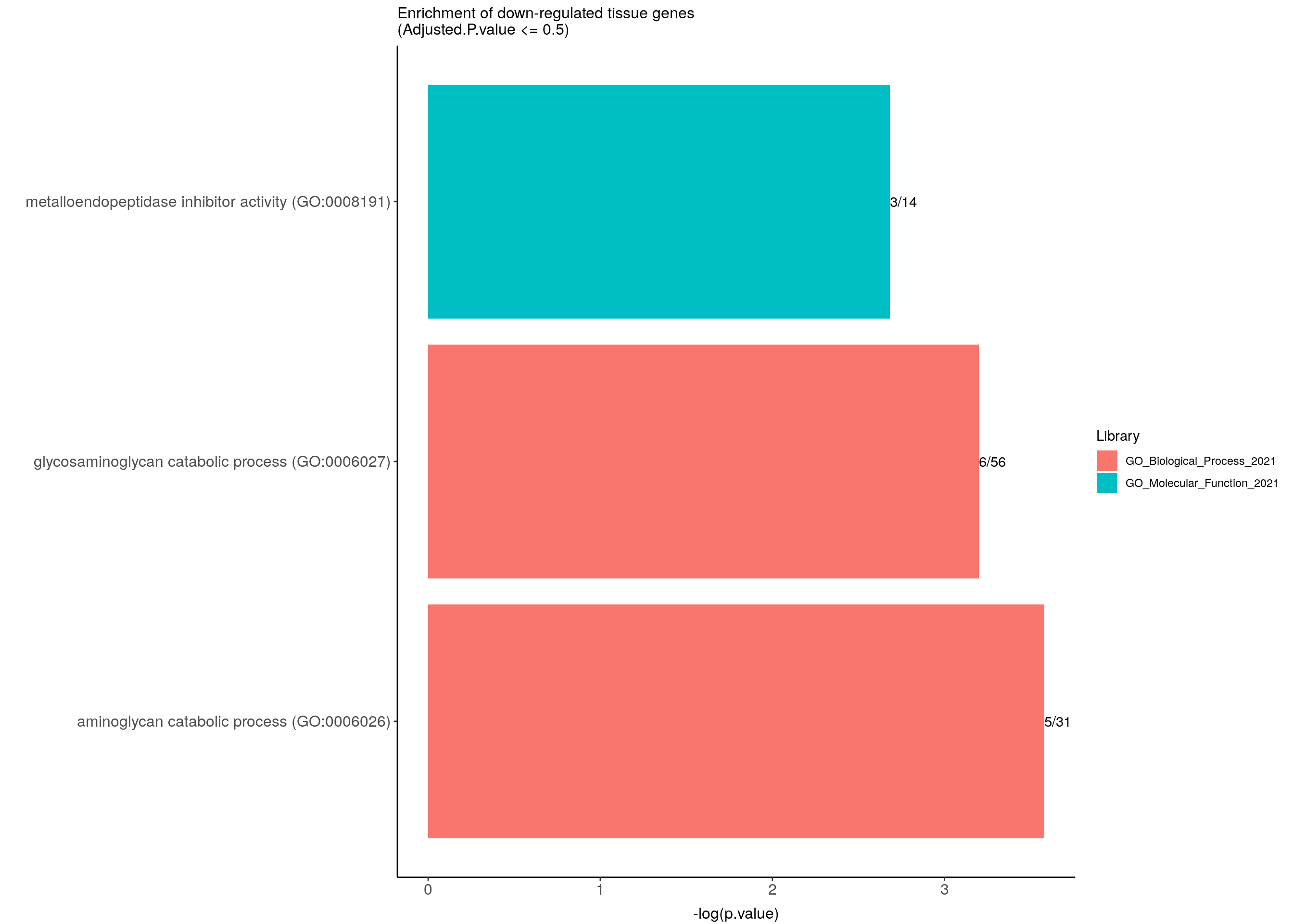
| Version | Author | Date |
|---|---|---|
| 50e8649 | xhyuo | 2022-10-13 |
sessionInfo()R version 4.0.3 (2020-10-10)
Platform: x86_64-pc-linux-gnu (64-bit)
Running under: Ubuntu 20.04.2 LTS
Matrix products: default
BLAS/LAPACK: /usr/lib/x86_64-linux-gnu/openblas-pthread/libopenblasp-r0.3.8.so
locale:
[1] LC_CTYPE=en_US.UTF-8 LC_NUMERIC=C
[3] LC_TIME=en_US.UTF-8 LC_COLLATE=en_US.UTF-8
[5] LC_MONETARY=en_US.UTF-8 LC_MESSAGES=C
[7] LC_PAPER=en_US.UTF-8 LC_NAME=C
[9] LC_ADDRESS=C LC_TELEPHONE=C
[11] LC_MEASUREMENT=en_US.UTF-8 LC_IDENTIFICATION=C
attached base packages:
[1] parallel stats4 stats graphics grDevices utils datasets
[8] methods base
other attached packages:
[1] sva_3.38.0 BiocParallel_1.24.1
[3] genefilter_1.72.1 mgcv_1.8-34
[5] nlme_3.1-152 ggplotify_0.0.5
[7] cowplot_1.1.1 enrichR_3.0
[9] DT_0.17 ggrepel_0.9.1
[11] pheatmap_1.0.12 DESeq2_1.30.1
[13] SummarizedExperiment_1.20.0 MatrixGenerics_1.2.1
[15] matrixStats_0.58.0 GenomicRanges_1.42.0
[17] GenomeInfoDb_1.26.7 RColorBrewer_1.1-2
[19] org.Mm.eg.db_3.12.0 AnnotationDbi_1.52.0
[21] IRanges_2.24.1 S4Vectors_0.28.1
[23] Biobase_2.50.0 BiocGenerics_0.36.1
[25] gplots_3.1.1 Glimma_2.0.0
[27] edgeR_3.32.1 limma_3.46.0
[29] forcats_0.5.1 dplyr_1.0.4
[31] purrr_0.3.4 readr_1.4.0
[33] tidyr_1.1.2 tibble_3.0.6
[35] ggplot2_3.3.3 tidyverse_1.3.0
[37] stringr_1.4.0 workflowr_1.6.2
loaded via a namespace (and not attached):
[1] colorspace_2.0-0 rjson_0.2.20 ellipsis_0.3.1
[4] rprojroot_2.0.2 XVector_0.30.0 fs_1.5.0
[7] rstudioapi_0.13 farver_2.0.3 bit64_4.0.5
[10] lubridate_1.7.9.2 xml2_1.3.2 splines_4.0.3
[13] cachem_1.0.4 geneplotter_1.68.0 knitr_1.31
[16] jsonlite_1.7.2 broom_0.7.4 annotate_1.68.0
[19] dbplyr_2.1.0 BiocManager_1.30.10 compiler_4.0.3
[22] httr_1.4.2 rvcheck_0.1.8 backports_1.2.1
[25] assertthat_0.2.1 Matrix_1.3-2 fastmap_1.1.0
[28] cli_2.3.0 later_1.1.0.1 htmltools_0.5.1.1
[31] tools_4.0.3 gtable_0.3.0 glue_1.4.2
[34] GenomeInfoDbData_1.2.4 Rcpp_1.0.6 cellranger_1.1.0
[37] vctrs_0.3.6 crosstalk_1.1.1 xfun_0.21
[40] rvest_0.3.6 lifecycle_1.0.0 gtools_3.8.2
[43] XML_3.99-0.5 zlibbioc_1.36.0 scales_1.1.1
[46] hms_1.0.0 promises_1.2.0.1 curl_4.3
[49] yaml_2.2.1 memoise_2.0.0 stringi_1.5.3
[52] RSQLite_2.2.3 highr_0.8 caTools_1.18.1
[55] rlang_1.0.2 pkgconfig_2.0.3 bitops_1.0-6
[58] evaluate_0.14 lattice_0.20-41 labeling_0.4.2
[61] htmlwidgets_1.5.3 bit_4.0.4 tidyselect_1.1.0
[64] magrittr_2.0.1 R6_2.5.0 generics_0.1.0
[67] DelayedArray_0.16.3 DBI_1.1.1 pillar_1.4.7
[70] haven_2.3.1 whisker_0.4 withr_2.4.1
[73] survival_3.2-7 RCurl_1.98-1.2 modelr_0.1.8
[76] crayon_1.4.1 KernSmooth_2.23-18 rmarkdown_2.6
[79] locfit_1.5-9.4 grid_4.0.3 readxl_1.3.1
[82] blob_1.2.1 git2r_0.28.0 reprex_1.0.0
[85] digest_0.6.27 xtable_1.8-4 httpuv_1.5.5
[88] gridGraphics_0.5-1 munsell_0.5.0 This R Markdown site was created with workflowr