Plot_DO_fentanyl
Hao He
2023-02-21
Last updated: 2023-02-21
Checks: 7 0
Knit directory: DO_Opioid/
This reproducible R Markdown analysis was created with workflowr (version 1.6.2). The Checks tab describes the reproducibility checks that were applied when the results were created. The Past versions tab lists the development history.
Great! Since the R Markdown file has been committed to the Git repository, you know the exact version of the code that produced these results.
Great job! The global environment was empty. Objects defined in the global environment can affect the analysis in your R Markdown file in unknown ways. For reproduciblity it’s best to always run the code in an empty environment.
The command set.seed(20200504) was run prior to running the code in the R Markdown file. Setting a seed ensures that any results that rely on randomness, e.g. subsampling or permutations, are reproducible.
Great job! Recording the operating system, R version, and package versions is critical for reproducibility.
Nice! There were no cached chunks for this analysis, so you can be confident that you successfully produced the results during this run.
Great job! Using relative paths to the files within your workflowr project makes it easier to run your code on other machines.
Great! You are using Git for version control. Tracking code development and connecting the code version to the results is critical for reproducibility.
The results in this page were generated with repository version 2200f95. See the Past versions tab to see a history of the changes made to the R Markdown and HTML files.
Note that you need to be careful to ensure that all relevant files for the analysis have been committed to Git prior to generating the results (you can use wflow_publish or wflow_git_commit). workflowr only checks the R Markdown file, but you know if there are other scripts or data files that it depends on. Below is the status of the Git repository when the results were generated:
Ignored files:
    Ignored:    .RData
    Ignored:    .Rhistory
    Ignored:    .Rproj.user/
    Ignored:    analysis/Picture1.png

Untracked files:
    Untracked:  Rplot_rz.png
    Untracked:  TIMBR.test.prop.bm.MN.RET.RData
    Untracked:  TIMBR.test.random.RData
    Untracked:  TIMBR.test.rz.transformed_TVb_ml.RData
    Untracked:  analysis/DDO_morphine1_second_set_69k.stdout
    Untracked:  analysis/DO_Fentanyl.R
    Untracked:  analysis/DO_Fentanyl.err
    Untracked:  analysis/DO_Fentanyl.out
    Untracked:  analysis/DO_Fentanyl.sh
    Untracked:  analysis/DO_Fentanyl_69k.R
    Untracked:  analysis/DO_Fentanyl_69k.err
    Untracked:  analysis/DO_Fentanyl_69k.out
    Untracked:  analysis/DO_Fentanyl_69k.sh
    Untracked:  analysis/DO_Fentanyl_Cohort2_GCTA_herit.R
    Untracked:  analysis/DO_Fentanyl_Cohort2_gemma.R
    Untracked:  analysis/DO_Fentanyl_Cohort2_mapping.R
    Untracked:  analysis/DO_Fentanyl_Cohort2_mapping.err
    Untracked:  analysis/DO_Fentanyl_Cohort2_mapping.out
    Untracked:  analysis/DO_Fentanyl_Cohort2_mapping.sh
    Untracked:  analysis/DO_Fentanyl_GCTA_herit.R
    Untracked:  analysis/DO_Fentanyl_alternate_metrics_69k.R
    Untracked:  analysis/DO_Fentanyl_alternate_metrics_69k.err
    Untracked:  analysis/DO_Fentanyl_alternate_metrics_69k.out
    Untracked:  analysis/DO_Fentanyl_alternate_metrics_69k.sh
    Untracked:  analysis/DO_Fentanyl_alternate_metrics_array.R
    Untracked:  analysis/DO_Fentanyl_alternate_metrics_array.err
    Untracked:  analysis/DO_Fentanyl_alternate_metrics_array.out
    Untracked:  analysis/DO_Fentanyl_alternate_metrics_array.sh
    Untracked:  analysis/DO_Fentanyl_array.R
    Untracked:  analysis/DO_Fentanyl_array.err
    Untracked:  analysis/DO_Fentanyl_array.out
    Untracked:  analysis/DO_Fentanyl_array.sh
    Untracked:  analysis/DO_Fentanyl_combining2Cohort_GCTA_herit.R
    Untracked:  analysis/DO_Fentanyl_combining2Cohort_gemma.R
    Untracked:  analysis/DO_Fentanyl_combining2Cohort_mapping.R
    Untracked:  analysis/DO_Fentanyl_combining2Cohort_mapping.err
    Untracked:  analysis/DO_Fentanyl_combining2Cohort_mapping.out
    Untracked:  analysis/DO_Fentanyl_combining2Cohort_mapping.sh
    Untracked:  analysis/DO_Fentanyl_combining2Cohort_mapping_CoxPH.R
    Untracked:  analysis/DO_Fentanyl_finalreport_to_plink.sh
    Untracked:  analysis/DO_Fentanyl_gemma.R
    Untracked:  analysis/DO_Fentanyl_gemma.err
    Untracked:  analysis/DO_Fentanyl_gemma.out
    Untracked:  analysis/DO_Fentanyl_gemma.sh
    Untracked:  analysis/DO_morphine1.R
    Untracked:  analysis/DO_morphine1.Rout
    Untracked:  analysis/DO_morphine1.sh
    Untracked:  analysis/DO_morphine1.stderr
    Untracked:  analysis/DO_morphine1.stdout
    Untracked:  analysis/DO_morphine1_SNP.R
    Untracked:  analysis/DO_morphine1_SNP.Rout
    Untracked:  analysis/DO_morphine1_SNP.sh
    Untracked:  analysis/DO_morphine1_SNP.stderr
    Untracked:  analysis/DO_morphine1_SNP.stdout
    Untracked:  analysis/DO_morphine1_combined.R
    Untracked:  analysis/DO_morphine1_combined.Rout
    Untracked:  analysis/DO_morphine1_combined.sh
    Untracked:  analysis/DO_morphine1_combined.stderr
    Untracked:  analysis/DO_morphine1_combined.stdout
    Untracked:  analysis/DO_morphine1_combined_69k.R
    Untracked:  analysis/DO_morphine1_combined_69k.Rout
    Untracked:  analysis/DO_morphine1_combined_69k.sh
    Untracked:  analysis/DO_morphine1_combined_69k.stderr
    Untracked:  analysis/DO_morphine1_combined_69k.stdout
    Untracked:  analysis/DO_morphine1_combined_69k_m2.R
    Untracked:  analysis/DO_morphine1_combined_69k_m2.Rout
    Untracked:  analysis/DO_morphine1_combined_69k_m2.sh
    Untracked:  analysis/DO_morphine1_combined_69k_m2.stderr
    Untracked:  analysis/DO_morphine1_combined_69k_m2.stdout
    Untracked:  analysis/DO_morphine1_combined_weight_DOB.R
    Untracked:  analysis/DO_morphine1_combined_weight_DOB.Rout
    Untracked:  analysis/DO_morphine1_combined_weight_DOB.err
    Untracked:  analysis/DO_morphine1_combined_weight_DOB.out
    Untracked:  analysis/DO_morphine1_combined_weight_DOB.sh
    Untracked:  analysis/DO_morphine1_combined_weight_DOB.stderr
    Untracked:  analysis/DO_morphine1_combined_weight_DOB.stdout
    Untracked:  analysis/DO_morphine1_combined_weight_age.R
    Untracked:  analysis/DO_morphine1_combined_weight_age.err
    Untracked:  analysis/DO_morphine1_combined_weight_age.out
    Untracked:  analysis/DO_morphine1_combined_weight_age.sh
    Untracked:  analysis/DO_morphine1_combined_weight_age_GAMMT.R
    Untracked:  analysis/DO_morphine1_combined_weight_age_GAMMT.err
    Untracked:  analysis/DO_morphine1_combined_weight_age_GAMMT.out
    Untracked:  analysis/DO_morphine1_combined_weight_age_GAMMT.sh
    Untracked:  analysis/DO_morphine1_combined_weight_age_GAMMT_chr19.R
    Untracked:  analysis/DO_morphine1_combined_weight_age_GAMMT_chr19.err
    Untracked:  analysis/DO_morphine1_combined_weight_age_GAMMT_chr19.out
    Untracked:  analysis/DO_morphine1_combined_weight_age_GAMMT_chr19.sh
    Untracked:  analysis/DO_morphine1_cph.R
    Untracked:  analysis/DO_morphine1_cph.Rout
    Untracked:  analysis/DO_morphine1_cph.sh
    Untracked:  analysis/DO_morphine1_second_set.R
    Untracked:  analysis/DO_morphine1_second_set.Rout
    Untracked:  analysis/DO_morphine1_second_set.sh
    Untracked:  analysis/DO_morphine1_second_set.stderr
    Untracked:  analysis/DO_morphine1_second_set.stdout
    Untracked:  analysis/DO_morphine1_second_set_69k.R
    Untracked:  analysis/DO_morphine1_second_set_69k.Rout
    Untracked:  analysis/DO_morphine1_second_set_69k.sh
    Untracked:  analysis/DO_morphine1_second_set_69k.stderr
    Untracked:  analysis/DO_morphine1_second_set_SNP.R
    Untracked:  analysis/DO_morphine1_second_set_SNP.Rout
    Untracked:  analysis/DO_morphine1_second_set_SNP.sh
    Untracked:  analysis/DO_morphine1_second_set_SNP.stderr
    Untracked:  analysis/DO_morphine1_second_set_SNP.stdout
    Untracked:  analysis/DO_morphine1_second_set_weight_DOB.R
    Untracked:  analysis/DO_morphine1_second_set_weight_DOB.Rout
    Untracked:  analysis/DO_morphine1_second_set_weight_DOB.err
    Untracked:  analysis/DO_morphine1_second_set_weight_DOB.out
    Untracked:  analysis/DO_morphine1_second_set_weight_DOB.sh
    Untracked:  analysis/DO_morphine1_second_set_weight_DOB.stderr
    Untracked:  analysis/DO_morphine1_second_set_weight_DOB.stdout
    Untracked:  analysis/DO_morphine1_second_set_weight_age.R
    Untracked:  analysis/DO_morphine1_second_set_weight_age.Rout
    Untracked:  analysis/DO_morphine1_second_set_weight_age.err
    Untracked:  analysis/DO_morphine1_second_set_weight_age.out
    Untracked:  analysis/DO_morphine1_second_set_weight_age.sh
    Untracked:  analysis/DO_morphine1_second_set_weight_age.stderr
    Untracked:  analysis/DO_morphine1_second_set_weight_age.stdout
    Untracked:  analysis/DO_morphine1_weight_DOB.R
    Untracked:  analysis/DO_morphine1_weight_DOB.sh
    Untracked:  analysis/DO_morphine1_weight_age.R
    Untracked:  analysis/DO_morphine1_weight_age.sh
    Untracked:  analysis/DO_morphine_gemma.R
    Untracked:  analysis/DO_morphine_gemma.err
    Untracked:  analysis/DO_morphine_gemma.out
    Untracked:  analysis/DO_morphine_gemma.sh
    Untracked:  analysis/DO_morphine_gemma_firstmin.R
    Untracked:  analysis/DO_morphine_gemma_firstmin.err
    Untracked:  analysis/DO_morphine_gemma_firstmin.out
    Untracked:  analysis/DO_morphine_gemma_firstmin.sh
    Untracked:  analysis/DO_morphine_gemma_withpermu.R
    Untracked:  analysis/DO_morphine_gemma_withpermu.err
    Untracked:  analysis/DO_morphine_gemma_withpermu.out
    Untracked:  analysis/DO_morphine_gemma_withpermu.sh
    Untracked:  analysis/DO_morphine_gemma_withpermu_firstbatch_min.depression.R
    Untracked:  analysis/DO_morphine_gemma_withpermu_firstbatch_min.depression.err
    Untracked:  analysis/DO_morphine_gemma_withpermu_firstbatch_min.depression.out
    Untracked:  analysis/DO_morphine_gemma_withpermu_firstbatch_min.depression.sh
    Untracked:  analysis/Plot_DO_morphine1_SNP.R
    Untracked:  analysis/Plot_DO_morphine1_SNP.Rout
    Untracked:  analysis/Plot_DO_morphine1_SNP.sh
    Untracked:  analysis/Plot_DO_morphine1_SNP.stderr
    Untracked:  analysis/Plot_DO_morphine1_SNP.stdout
    Untracked:  analysis/Plot_DO_morphine1_second_set_SNP.R
    Untracked:  analysis/Plot_DO_morphine1_second_set_SNP.Rout
    Untracked:  analysis/Plot_DO_morphine1_second_set_SNP.sh
    Untracked:  analysis/Plot_DO_morphine1_second_set_SNP.stderr
    Untracked:  analysis/Plot_DO_morphine1_second_set_SNP.stdout
    Untracked:  analysis/download_GSE100356_sra.sh
    Untracked:  analysis/fentanyl_2cohorts_coxph.R
    Untracked:  analysis/fentanyl_2cohorts_coxph.err
    Untracked:  analysis/fentanyl_2cohorts_coxph.out
    Untracked:  analysis/fentanyl_2cohorts_coxph.sh
    Untracked:  analysis/fentanyl_scanone.cph.R
    Untracked:  analysis/fentanyl_scanone.cph.err
    Untracked:  analysis/fentanyl_scanone.cph.out
    Untracked:  analysis/fentanyl_scanone.cph.sh
    Untracked:  analysis/geo_rnaseq.R
    Untracked:  analysis/heritability_first_second_batch.R
    Untracked:  analysis/nf-rnaseq-b6.R
    Untracked:  analysis/plot_fentanyl_2cohorts_coxph.R
    Untracked:  analysis/scripts/
    Untracked:  analysis/tibmr.R
    Untracked:  analysis/timbr_demo.R
    Untracked:  analysis/workflow_proc.R
    Untracked:  analysis/workflow_proc.sh
    Untracked:  analysis/workflow_proc.stderr
    Untracked:  analysis/workflow_proc.stdout
    Untracked:  analysis/x.R
    Untracked:  code/cfw/
    Untracked:  code/gemma_plot.R
    Untracked:  code/process.sanger.snp.R
    Untracked:  code/reconst_utils.R
    Untracked:  data/69k_grid_pgmap.RData
    Untracked:  data/Composite Post Kevins Program Group 2 Fentanyl Prepped for Hao.xlsx
    Untracked:  data/DO_WBP_Data_JAB_to_map.xlsx
    Untracked:  data/Fentanyl_alternate_metrics.xlsx
    Untracked:  data/FinalReport/
    Untracked:  data/GM/
    Untracked:  data/GM_covar.csv
    Untracked:  data/GM_covar_07092018_morphine.csv
    Untracked:  data/Jackson_Lab_Bubier_MURGIGV01/
    Untracked:  data/MPD_Upload_October.csv
    Untracked:  data/MPD_Upload_October_updated_sex.csv
    Untracked:  data/Master Fentanyl DO Study Sheet.xlsx
    Untracked:  data/MasterMorphine Second Set DO w DOB2.xlsx
    Untracked:  data/MasterMorphine Second Set DO.xlsx
    Untracked:  data/Morphine CC DO mice Updated with Published inbred strains.csv
    Untracked:  data/Morphine_CC_DO_mice_Updated_with_Published_inbred_strains.csv
    Untracked:  data/cc_variants.sqlite
    Untracked:  data/combined/
    Untracked:  data/fentanyl/
    Untracked:  data/fentanyl2/
    Untracked:  data/fentanyl_1_2/
    Untracked:  data/fentanyl_2cohorts_coxph_data.Rdata
    Untracked:  data/first/
    Untracked:  data/founder_geno.csv
    Untracked:  data/genetic_map.csv
    Untracked:  data/gm.json
    Untracked:  data/gwas.sh
    Untracked:  data/marker_grid_0.02cM_plus.txt
    Untracked:  data/mouse_genes_mgi.sqlite
    Untracked:  data/pheno.csv
    Untracked:  data/pheno_qtl2.csv
    Untracked:  data/pheno_qtl2_07092018_morphine.csv
    Untracked:  data/pheno_qtl2_w_dob.csv
    Untracked:  data/physical_map.csv
    Untracked:  data/rnaseq/
    Untracked:  data/sample_geno.csv
    Untracked:  data/second/
    Untracked:  figure/
    Untracked:  glimma-plots/
    Untracked:  output/DO_Fentanyl_Cohort2_MinDepressionRR_coefplot.pdf
    Untracked:  output/DO_Fentanyl_Cohort2_MinDepressionRR_coefplot_blup.pdf
    Untracked:  output/DO_Fentanyl_Cohort2_RRDepressionRateHrSLOPE_coefplot.pdf
    Untracked:  output/DO_Fentanyl_Cohort2_RRRecoveryRateHrSLOPE_coefplot.pdf
    Untracked:  output/DO_Fentanyl_Cohort2_RRRecoveryRateHrSLOPE_coefplot_blup.pdf
    Untracked:  output/DO_Fentanyl_Cohort2_StartofRecoveryHr_coefplot.pdf
    Untracked:  output/DO_Fentanyl_Cohort2_StartofRecoveryHr_coefplot_blup.pdf
    Untracked:  output/DO_Fentanyl_Cohort2_Statusbin_coefplot.pdf
    Untracked:  output/DO_Fentanyl_Cohort2_Statusbin_coefplot_blup.pdf
    Untracked:  output/DO_Fentanyl_Cohort2_SteadyStateDepressionDurationHrINTERVAL_coefplot.pdf
    Untracked:  output/DO_Fentanyl_Cohort2_TimetoDead(Hr)_coefplot.pdf
    Untracked:  output/DO_Fentanyl_Cohort2_TimetoDeadHr_coefplot.pdf
    Untracked:  output/DO_Fentanyl_Cohort2_TimetoDeadHr_coefplot_blup.pdf
    Untracked:  output/DO_Fentanyl_Cohort2_TimetoProjectedRecoveryHr_coefplot.pdf
    Untracked:  output/DO_Fentanyl_Cohort2_TimetoProjectedRecoveryHr_coefplot_blup.pdf
    Untracked:  output/DO_Fentanyl_Cohort2_TimetoSteadyRRDepression(Hr)_coefplot.pdf
    Untracked:  output/DO_Fentanyl_Cohort2_TimetoSteadyRRDepressionHr_coefplot.pdf
    Untracked:  output/DO_Fentanyl_Cohort2_TimetoSteadyRRDepressionHr_coefplot_blup.pdf
    Untracked:  output/DO_Fentanyl_Cohort2_TimetoThresholdRecoveryHr_coefplot.pdf
    Untracked:  output/DO_Fentanyl_Cohort2_TimetoThresholdRecoveryHr_coefplot_blup.pdf
    Untracked:  output/DO_morphine_Min.depression.png
    Untracked:  output/DO_morphine_Min.depression22222_violin_chr5.pdf
    Untracked:  output/DO_morphine_Min.depression_coefplot.pdf
    Untracked:  output/DO_morphine_Min.depression_coefplot_blup.pdf
    Untracked:  output/DO_morphine_Min.depression_coefplot_blup_chr5.png
    Untracked:  output/DO_morphine_Min.depression_coefplot_blup_chrX.png
    Untracked:  output/DO_morphine_Min.depression_coefplot_chr5.png
    Untracked:  output/DO_morphine_Min.depression_coefplot_chrX.png
    Untracked:  output/DO_morphine_Min.depression_peak_genes_chr5.png
    Untracked:  output/DO_morphine_Min.depression_violin_chr5.png
    Untracked:  output/DO_morphine_Recovery.Time.png
    Untracked:  output/DO_morphine_Recovery.Time_coefplot.pdf
    Untracked:  output/DO_morphine_Recovery.Time_coefplot_blup.pdf
    Untracked:  output/DO_morphine_Recovery.Time_coefplot_blup_chr11.png
    Untracked:  output/DO_morphine_Recovery.Time_coefplot_blup_chr4.png
    Untracked:  output/DO_morphine_Recovery.Time_coefplot_blup_chr7.png
    Untracked:  output/DO_morphine_Recovery.Time_coefplot_blup_chr9.png
    Untracked:  output/DO_morphine_Recovery.Time_coefplot_chr11.png
    Untracked:  output/DO_morphine_Recovery.Time_coefplot_chr4.png
    Untracked:  output/DO_morphine_Recovery.Time_coefplot_chr7.png
    Untracked:  output/DO_morphine_Recovery.Time_coefplot_chr9.png
    Untracked:  output/DO_morphine_Status_bin.png
    Untracked:  output/DO_morphine_Status_bin_coefplot.pdf
    Untracked:  output/DO_morphine_Status_bin_coefplot_blup.pdf
    Untracked:  output/DO_morphine_Survival.Time.png
    Untracked:  output/DO_morphine_Survival.Time_coefplot.pdf
    Untracked:  output/DO_morphine_Survival.Time_coefplot_blup.pdf
    Untracked:  output/DO_morphine_Survival.Time_coefplot_blup_chr17.png
    Untracked:  output/DO_morphine_Survival.Time_coefplot_blup_chr8.png
    Untracked:  output/DO_morphine_Survival.Time_coefplot_chr17.png
    Untracked:  output/DO_morphine_Survival.Time_coefplot_chr8.png
    Untracked:  output/DO_morphine_combine_batch_peak_violin.pdf
    Untracked:  output/DO_morphine_combined_69k_m2_Min.depression.png
    Untracked:  output/DO_morphine_combined_69k_m2_Min.depression_coefplot.pdf
    Untracked:  output/DO_morphine_combined_69k_m2_Min.depression_coefplot_blup.pdf
    Untracked:  output/DO_morphine_combined_69k_m2_Recovery.Time.png
    Untracked:  output/DO_morphine_combined_69k_m2_Recovery.Time_coefplot.pdf
    Untracked:  output/DO_morphine_combined_69k_m2_Recovery.Time_coefplot_blup.pdf
    Untracked:  output/DO_morphine_combined_69k_m2_Status_bin.png
    Untracked:  output/DO_morphine_combined_69k_m2_Status_bin_coefplot.pdf
    Untracked:  output/DO_morphine_combined_69k_m2_Status_bin_coefplot_blup.pdf
    Untracked:  output/DO_morphine_combined_69k_m2_Survival.Time.png
    Untracked:  output/DO_morphine_combined_69k_m2_Survival.Time_coefplot.pdf
    Untracked:  output/DO_morphine_combined_69k_m2_Survival.Time_coefplot_blup.pdf
    Untracked:  output/DO_morphine_coxph_24hrs_kinship_QTL.png
    Untracked:  output/DO_morphine_cphout.RData
    Untracked:  output/DO_morphine_first_batch_peak_in_second_batch_violin.pdf
    Untracked:  output/DO_morphine_first_batch_peak_in_second_batch_violin_sidebyside.pdf
    Untracked:  output/DO_morphine_first_batch_peak_violin.pdf
    Untracked:  output/DO_morphine_operm.cph.RData
    Untracked:  output/DO_morphine_second_batch_on_first_batch_peak_violin.pdf
    Untracked:  output/DO_morphine_second_batch_peak_ch6surv_on_first_batchviolin.pdf
    Untracked:  output/DO_morphine_second_batch_peak_ch6surv_on_first_batchviolin2.pdf
    Untracked:  output/DO_morphine_second_batch_peak_in_first_batch_violin.pdf
    Untracked:  output/DO_morphine_second_batch_peak_in_first_batch_violin_sidebyside.pdf
    Untracked:  output/DO_morphine_second_batch_peak_violin.pdf
    Untracked:  output/DO_morphine_secondbatch_69k_Min.depression.png
    Untracked:  output/DO_morphine_secondbatch_69k_Min.depression_coefplot.pdf
    Untracked:  output/DO_morphine_secondbatch_69k_Min.depression_coefplot_blup.pdf
    Untracked:  output/DO_morphine_secondbatch_69k_Recovery.Time.png
    Untracked:  output/DO_morphine_secondbatch_69k_Recovery.Time_coefplot.pdf
    Untracked:  output/DO_morphine_secondbatch_69k_Recovery.Time_coefplot_blup.pdf
    Untracked:  output/DO_morphine_secondbatch_69k_Status_bin.png
    Untracked:  output/DO_morphine_secondbatch_69k_Status_bin_coefplot.pdf
    Untracked:  output/DO_morphine_secondbatch_69k_Status_bin_coefplot_blup.pdf
    Untracked:  output/DO_morphine_secondbatch_69k_Survival.Time.png
    Untracked:  output/DO_morphine_secondbatch_69k_Survival.Time_coefplot.pdf
    Untracked:  output/DO_morphine_secondbatch_69k_Survival.Time_coefplot_blup.pdf
    Untracked:  output/DO_morphine_secondbatch_Min.depression.png
    Untracked:  output/DO_morphine_secondbatch_Min.depression_coefplot.pdf
    Untracked:  output/DO_morphine_secondbatch_Min.depression_coefplot_blup.pdf
    Untracked:  output/DO_morphine_secondbatch_Recovery.Time.png
    Untracked:  output/DO_morphine_secondbatch_Recovery.Time_coefplot.pdf
    Untracked:  output/DO_morphine_secondbatch_Recovery.Time_coefplot_blup.pdf
    Untracked:  output/DO_morphine_secondbatch_Status_bin.png
    Untracked:  output/DO_morphine_secondbatch_Status_bin_coefplot.pdf
    Untracked:  output/DO_morphine_secondbatch_Status_bin_coefplot_blup.pdf
    Untracked:  output/DO_morphine_secondbatch_Survival.Time.png
    Untracked:  output/DO_morphine_secondbatch_Survival.Time_coefplot.pdf
    Untracked:  output/DO_morphine_secondbatch_Survival.Time_coefplot_blup.pdf
    Untracked:  output/Fentanyl/
    Untracked:  output/KPNA3.pdf
    Untracked:  output/SSC4D.pdf
    Untracked:  output/TIMBR.test.RData
    Untracked:  output/apr_69kchr_combined.RData
    Untracked:  output/apr_69kchr_k_loco_combined.rds
    Untracked:  output/apr_69kchr_second_set.RData
    Untracked:  output/combine_batch_variation.RData
    Untracked:  output/combined_gm.RData
    Untracked:  output/combined_gm.k_loco.rds
    Untracked:  output/combined_gm.k_overall.rds
    Untracked:  output/combined_gm.probs_8state.rds
    Untracked:  output/coxph/
    Untracked:  output/do.morphine.RData
    Untracked:  output/do.morphine.k_loco.rds
    Untracked:  output/do.morphine.probs_36state.rds
    Untracked:  output/do.morphine.probs_8state.rds
    Untracked:  output/do_Fentanyl_combine2cohort_MeanDepressionBR_coefplot.pdf
    Untracked:  output/do_Fentanyl_combine2cohort_MeanDepressionBR_coefplot_blup.pdf
    Untracked:  output/do_Fentanyl_combine2cohort_MinDepressionBR_coefplot.pdf
    Untracked:  output/do_Fentanyl_combine2cohort_MinDepressionBR_coefplot_blup.pdf
    Untracked:  output/do_Fentanyl_combine2cohort_MinDepressionRR_coefplot.pdf
    Untracked:  output/do_Fentanyl_combine2cohort_MinDepressionRR_coefplot_blup.pdf
    Untracked:  output/do_Fentanyl_combine2cohort_RRRecoveryRateHr_coefplot.pdf
    Untracked:  output/do_Fentanyl_combine2cohort_RRRecoveryRateHr_coefplot_blup.pdf
    Untracked:  output/do_Fentanyl_combine2cohort_StartofRecoveryHr_coefplot.pdf
    Untracked:  output/do_Fentanyl_combine2cohort_StartofRecoveryHr_coefplot_blup.pdf
    Untracked:  output/do_Fentanyl_combine2cohort_Statusbin_coefplot.pdf
    Untracked:  output/do_Fentanyl_combine2cohort_Statusbin_coefplot_blup.pdf
    Untracked:  output/do_Fentanyl_combine2cohort_SteadyStateDepressionDurationHr_coefplot.pdf
    Untracked:  output/do_Fentanyl_combine2cohort_SteadyStateDepressionDurationHr_coefplot_blup.pdf
    Untracked:  output/do_Fentanyl_combine2cohort_SurvivalTime_coefplot.pdf
    Untracked:  output/do_Fentanyl_combine2cohort_SurvivalTime_coefplot_blup.pdf
    Untracked:  output/do_Fentanyl_combine2cohort_TimetoDeadHr_coefplot.pdf
    Untracked:  output/do_Fentanyl_combine2cohort_TimetoDeadHr_coefplot_blup.pdf
    Untracked:  output/do_Fentanyl_combine2cohort_TimetoMostlyDeadHr_coefplot.pdf
    Untracked:  output/do_Fentanyl_combine2cohort_TimetoMostlyDeadHr_coefplot_blup.pdf
    Untracked:  output/do_Fentanyl_combine2cohort_TimetoProjectedRecoveryHr_coefplot.pdf
    Untracked:  output/do_Fentanyl_combine2cohort_TimetoProjectedRecoveryHr_coefplot_blup.pdf
    Untracked:  output/do_Fentanyl_combine2cohort_TimetoRecoveryHr_coefplot.pdf
    Untracked:  output/do_Fentanyl_combine2cohort_TimetoRecoveryHr_coefplot_blup.pdf
    Untracked:  output/first_batch_variation.RData
    Untracked:  output/first_second_survival_peak_chr.xlsx
    Untracked:  output/hsq_1_first_batch_herit_qtl2.RData
    Untracked:  output/hsq_2_second_batch_herit_qtl2.RData
    Untracked:  output/old_temp/
    Untracked:  output/pr_69kchr_combined.RData
    Untracked:  output/pr_69kchr_second_set.RData
    Untracked:  output/qtl.morphine.69k.out.combined.RData
    Untracked:  output/qtl.morphine.69k.out.combined_m2.RData
    Untracked:  output/qtl.morphine.69k.out.second_set.RData
    Untracked:  output/qtl.morphine.operm.RData
    Untracked:  output/qtl.morphine.out.RData
    Untracked:  output/qtl.morphine.out.combined_gm.RData
    Untracked:  output/qtl.morphine.out.combined_gm.female.RData
    Untracked:  output/qtl.morphine.out.combined_gm.male.RData
    Untracked:  output/qtl.morphine.out.combined_weight_DOB.RData
    Untracked:  output/qtl.morphine.out.combined_weight_age.RData
    Untracked:  output/qtl.morphine.out.female.RData
    Untracked:  output/qtl.morphine.out.male.RData
    Untracked:  output/qtl.morphine.out.second_set.RData
    Untracked:  output/qtl.morphine.out.second_set.female.RData
    Untracked:  output/qtl.morphine.out.second_set.male.RData
    Untracked:  output/qtl.morphine.out.second_set.weight_DOB.RData
    Untracked:  output/qtl.morphine.out.second_set.weight_age.RData
    Untracked:  output/qtl.morphine.out.weight_DOB.RData
    Untracked:  output/qtl.morphine.out.weight_age.RData
    Untracked:  output/qtl.morphine1.snpout.RData
    Untracked:  output/qtl.morphine2.snpout.RData
    Untracked:  output/second_batch_pheno.csv
    Untracked:  output/second_batch_variation.RData
    Untracked:  output/second_set_apr_69kchr_k_loco.rds
    Untracked:  output/second_set_gm.RData
    Untracked:  output/second_set_gm.k_loco.rds
    Untracked:  output/second_set_gm.probs_36state.rds
    Untracked:  output/second_set_gm.probs_8state.rds
    Untracked:  output/topSNP_chr5_mindepression.csv
    Untracked:  output/zoompeak_Min.depression_9.pdf
    Untracked:  output/zoompeak_Recovery.Time_16.pdf
    Untracked:  output/zoompeak_Status_bin_11.pdf
    Untracked:  output/zoompeak_Survival.Time_1.pdf
    Untracked:  output/zoompeak_fentanyl_Survival.Time_2.pdf
    Untracked:  sra-tools_v2.10.7.sif

Unstaged changes:
    Modified:   _workflowr.yml
    Modified:   analysis/marker_violin.Rmd
Note that any generated files, e.g. HTML, png, CSS, etc., are not included in this status report because it is ok for generated content to have uncommitted changes.
These are the previous versions of the repository in which changes were made to the R Markdown (analysis/Plot_DO_fentanyl.Rmd) and HTML (docs/Plot_DO_fentanyl.html) files. If you’ve configured a remote Git repository (see ?wflow_git_remote), click on the hyperlinks in the table below to view the files as they were in that past version.
| File | Version | Author | Date | Message |
|---|---|---|---|---|
| Rmd | 2200f95 | xhyuo | 2023-02-21 | update with sex specific Fentanyl plot |
| html | 8611541 | xhyuo | 2023-02-21 | Build site. |
| Rmd | d1a7028 | xhyuo | 2023-02-21 | update with sex specific Fentanyl |
| html | fd4dc88 | xhyuo | 2023-01-11 | Build site. |
| Rmd | aff7cd2 | xhyuo | 2023-01-11 | update with histogram |
| html | 3f3ae81 | xhyuo | 2021-11-15 | Build site. |
| Rmd | 5aceaae | xhyuo | 2021-11-15 | update_insp_flow_and_exp_flow |
| html | 7315d27 | xhyuo | 2021-10-22 | Build site. |
| Rmd | 3aa52ec | xhyuo | 2021-10-22 | add phenotype update qtl results and gemma |
| html | 9b57b94 | xhyuo | 2021-10-22 | Build site. |
| Rmd | 3e14cfa | xhyuo | 2021-10-22 | add phenotype update qtl results and gemma |
| Rmd | 956ed45 | xhyuo | 2021-10-22 | add phenotype update qtl results and gemma |
| html | 10ccb55 | xhyuo | 2021-09-19 | Build site. |
| Rmd | 9a36460 | xhyuo | 2021-09-19 | update id and qtl results and gemma |
| html | 3f2fa84 | xhyuo | 2021-09-06 | Build site. |
| Rmd | 95af54d | xhyuo | 2021-09-06 | fentanyl |
Last update: 2023-02-21
loading libraries
library(ggplot2)
library(gridExtra)
library(GGally)
library(parallel)
library(qtl2)
library(parallel)
library(survival)
library(regress)
library(abind)
library(openxlsx)
library(tidyverse)
library(cowplot)
library(furrr)
library(patchwork)
library(qtl)
theme_set(theme_cowplot())
source("code/gemma_plot.R")
source("code/cfw/R/gemma.R")

rz.transform <- function(y) {
  rankY=rank(y, ties.method="average", na.last="keep")
  rzT=qnorm(rankY/(length(na.exclude(rankY))+1))
  return(rzT)
}

Pvaltolod <- function(p){
  if(p == 0) p = 1e-10
  y = ifelse(p >= 0.5, 0, qchisq(1-2*p, df=1)/(2*log(10)))
  y
}

load("code/do.colors.RData")
Read phenotype data
# Read phenotype data -----------------------------------------------------
do.pheno <- read.xlsx("data/Master Fentanyl DO Study Sheet.xlsx", sheet = 1,
                      rows = 1:399, na.strings = "NaN", detectDates = TRUE)
#second 31009 is really 31109
do.pheno[do.pheno$ID == 31009 & do.pheno$File == 20210519, "ID"] = 31109
#remove zombie mice
do.pheno <- do.pheno %>%
  dplyr::filter(is.na(Censor)) %>%
  dplyr::rename(.,
                Min.depression = 9,
                Survival.Time  = 10,
                Recovery.Time  = 11) %>%
  dplyr::mutate(Status_bin = ifelse(Survival == "ALIVE", 1, 0)) %>%
  dplyr::mutate(ID = as.character(ID)) %>%
  dplyr::arrange(ID, desc(File)) %>%
  dplyr::distinct(ID, .keep_all = TRUE)
#wsp file
do.wsp <- read.xlsx("data/DO_WBP_Data_JAB_to_map.xlsx", sheet = 1)
colnames(do.wsp) <- str_replace(colnames(do.wsp), "\\.", "_")
colnames(do.wsp) <- str_replace(colnames(do.wsp), "\\(", "_")
colnames(do.wsp) <- str_replace(colnames(do.wsp), "\\)", "")
colnames(do.wsp) <- str_replace(colnames(do.wsp), "\\/", "_")
do.wsp$Mouse_ID <- as.character(do.wsp$Mouse_ID)
do.wsp <- distinct(do.wsp, Mouse_ID, .keep_all = TRUE)
#merge with do.pheno
do.pheno <- left_join(do.pheno, do.wsp, by = c("ID" = "Mouse_ID"))

# Read genotype data -----------------------------------------------------------
load("data/Jackson_Lab_Bubier_MURGIGV01/gm_DO395_qc_newid.RData")#gm_after_qc
overlap.id  = intersect(ind_ids(gm_after_qc), do.pheno$ID)

#update MPD sex
mpd <- read.csv("data/MPD_Upload_October.csv", header = TRUE)
mpd <- mpd %>%
  mutate(Mouse.ID = as.character(Mouse.ID)) %>%
  left_join(do.pheno[,2:3], by = c("Mouse.ID" = "ID")) %>%
  left_join(gm_after_qc$covar[, c(2,4)], by = c("Mouse.ID" = "name")) %>%
  mutate(Sex.y = ifelse(is.na(Sex.y), "", Sex.y)) %>%
  tidyr::unite("Sex", Sex.x, Sex.y, sep = "", remove = TRUE) %>%
  mutate(Sex = ifelse(Sex == "", sex, Sex)) %>%
  select(-sex)

#update insp_flow and exp_flow
do.pheno <- do.pheno %>%
  select(-c("insp_flow", "exp_flow")) %>%
  left_join(mpd[, c("Mouse.ID", "insp_flow", "exp_flow")], by = c("ID" = "Mouse.ID"))

#subset
gm = gm_after_qc[overlap.id, ]
do.pheno = do.pheno[do.pheno$ID %in% overlap.id, ]
do.pheno = do.pheno[match(ind_ids(gm), do.pheno$ID) , ]
rownames(do.pheno) = do.pheno$ID
all.equal(ind_ids(gm), do.pheno$ID)
# [1] TRUE

#boxplot on the raw data------------
#survival time
surv <- do.pheno[,c(2,3,10)]
surv <- surv[complete.cases(surv), ]
p1 <- ggplot(surv, aes(x=Sex, y=Survival.Time, group = Sex, fill = Sex, alpha = 0.9)) +
  geom_boxplot(show.legend = F , outlier.size = 1.5, notchwidth = 0.85) +
  geom_jitter(color="black", size=0.8, alpha=0.9) +
  scale_fill_brewer(palette="Blues") +
  ylab("Survival Time") +
  xlab("Sex") +
  labs(fill = "") +
  theme(legend.position = "none",
        panel.grid.major = element_blank(),
        panel.grid.minor = element_blank(),
        panel.background = element_blank(),
        axis.line = element_line(colour = "black"),
        text = element_text(size=21),
        axis.title=element_text(size=21)) +
  guides(shape = guide_legend(override.aes = list(size = 12)))
p1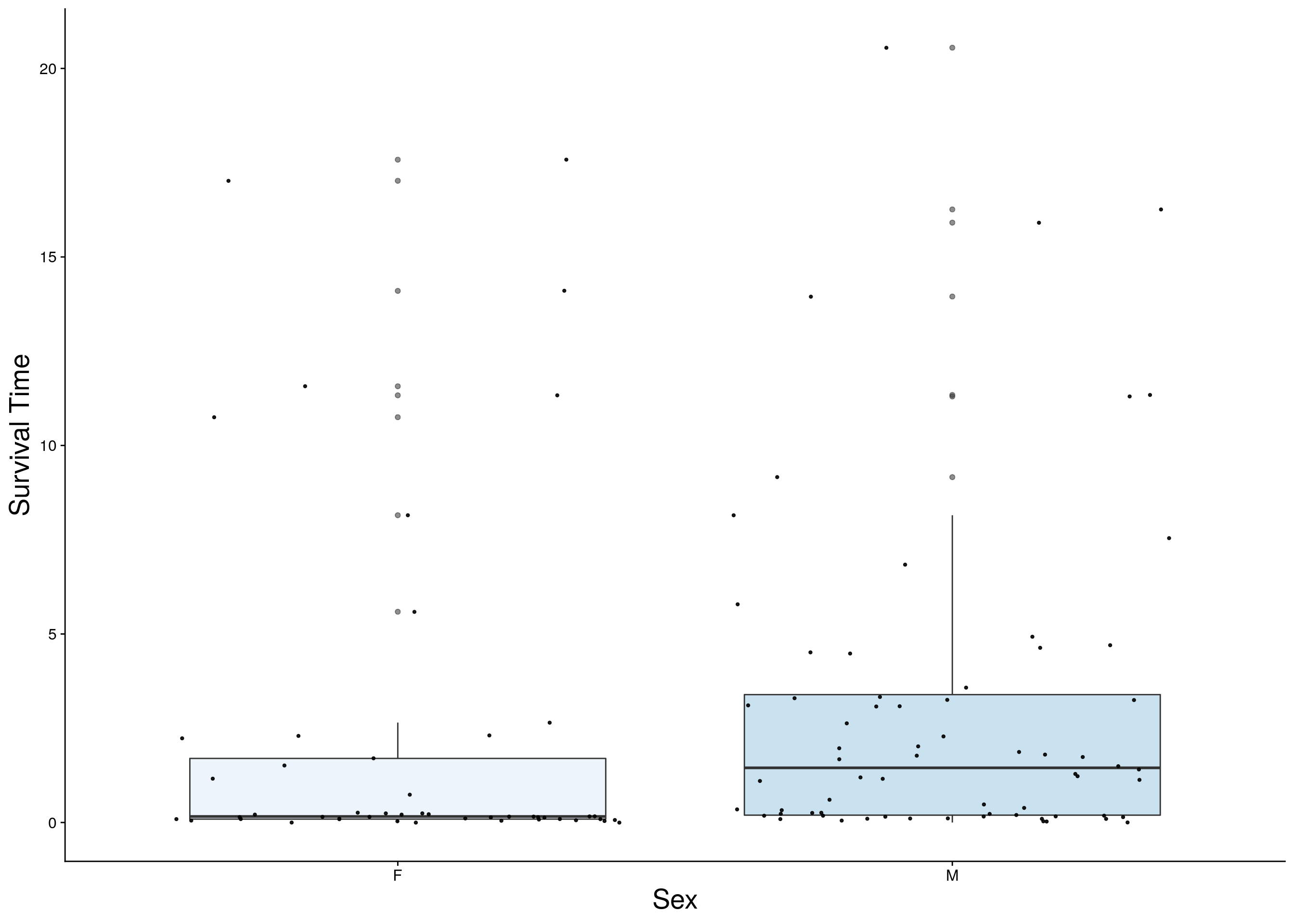
reco <- do.pheno[,c(2,3,11)]
reco <- reco[complete.cases(reco), ]
p2 <- ggplot(reco, aes(x=Sex, y=Recovery.Time, group = Sex, fill = Sex, alpha = 0.9)) +
  geom_boxplot(show.legend = F , outlier.size = 1.5, notchwidth = 0.85) +
  geom_jitter(color="black", size=0.8, alpha=0.9) +
  scale_fill_brewer(palette="Blues") +
  ylab("Recovery Time") +
  xlab("Sex") +
  labs(fill = "") +
  theme(legend.position = "none",
        panel.grid.major = element_blank(),
        panel.grid.minor = element_blank(),
        panel.background = element_blank(),
        axis.line = element_line(colour = "black"),
        text = element_text(size=21),
        axis.title=element_text(size=21)) +
  guides(shape = guide_legend(override.aes = list(size = 12)))
p2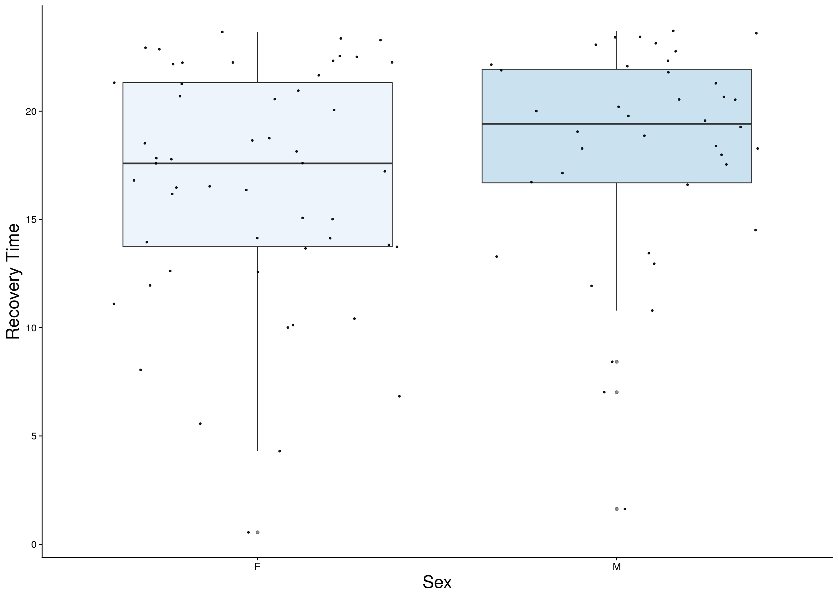
dep <- do.pheno[,c(2,3,9)]
dep <- dep[complete.cases(dep), ]
p3 <- ggplot(dep, aes(x=Sex, y=Min.depression, group = Sex, fill = Sex, alpha = 0.9)) +
  geom_boxplot(show.legend = F , outlier.size = 1.5, notchwidth = 0.85) +
  geom_jitter(color="black", size=0.8, alpha=0.9) +
  scale_fill_brewer(palette="Blues") +
  ylab("Min depression") +
  xlab("Sex") +
  labs(fill = "") +
  theme(legend.position = "none",
        panel.grid.major = element_blank(),
        panel.grid.minor = element_blank(),
        panel.background = element_blank(),
        axis.line = element_line(colour = "black"),
        text = element_text(size=21),
        axis.title=element_text(size=21)) +
  guides(shape = guide_legend(override.aes = list(size = 12)))
p3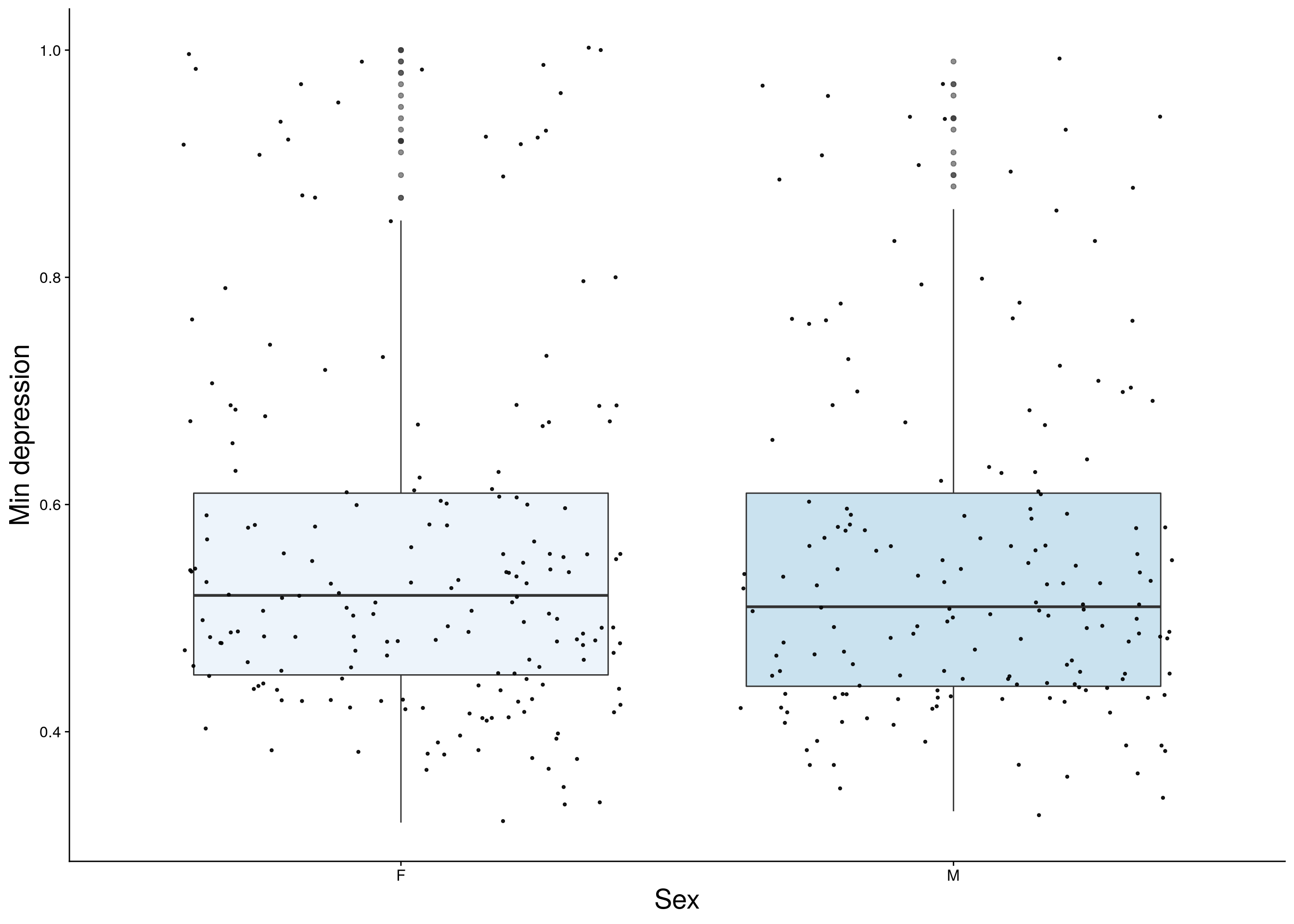
#histogram
a <- ggplot(data=do.pheno, aes(Survival.Time)) +
  geom_histogram() +
  ylab("Number of DO mice") + xlab("Survival Time (h)") +
  theme(panel.grid.major = element_blank(), panel.grid.minor = element_blank(),
        panel.background = element_blank(), axis.line = element_line(colour = "black"),
        text = element_text(size=21))
print(a)
# Warning: Removed 251 rows containing non-finite values (stat_bin).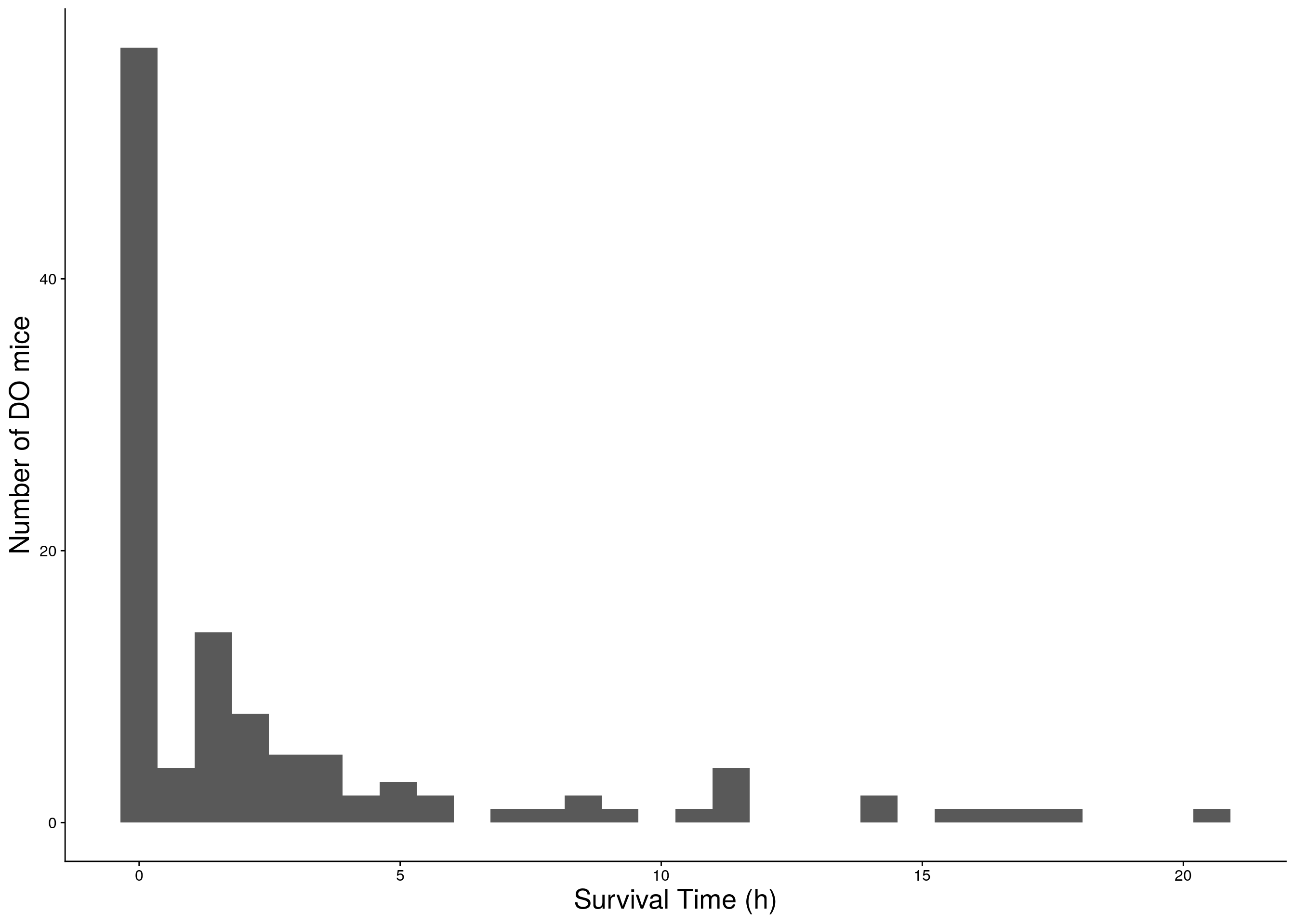
b <- ggplot(data=do.pheno, aes(Recovery.Time)) +
  geom_histogram() +
  ylab("Number of DO mice") + xlab("Recovery Time (h)") +
  theme(panel.grid.major = element_blank(), panel.grid.minor = element_blank(),
        panel.background = element_blank(), axis.line = element_line(colour = "black"),
        text = element_text(size=21))
print(b)
# Warning: Removed 275 rows containing non-finite values (stat_bin).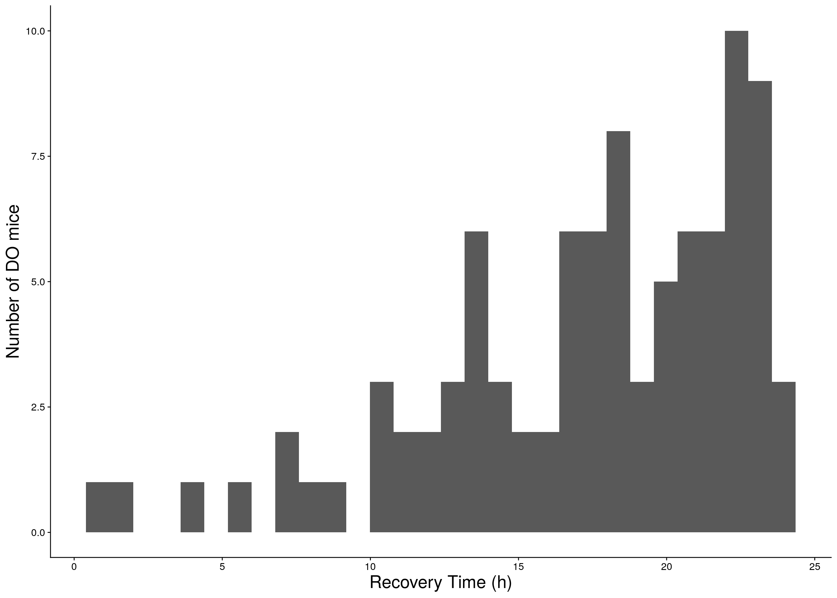
c <- ggplot(data=do.pheno, aes(Min.depression)) +
  geom_histogram() +
  ylab("Number of DO mice") + xlab("Respiratory Depression (% of baseline)") +
  theme(panel.grid.major = element_blank(), panel.grid.minor = element_blank(),
        panel.background = element_blank(), axis.line = element_line(colour = "black"),
        text = element_text(size=21))
print(c)
# Warning: Removed 12 rows containing non-finite values (stat_bin).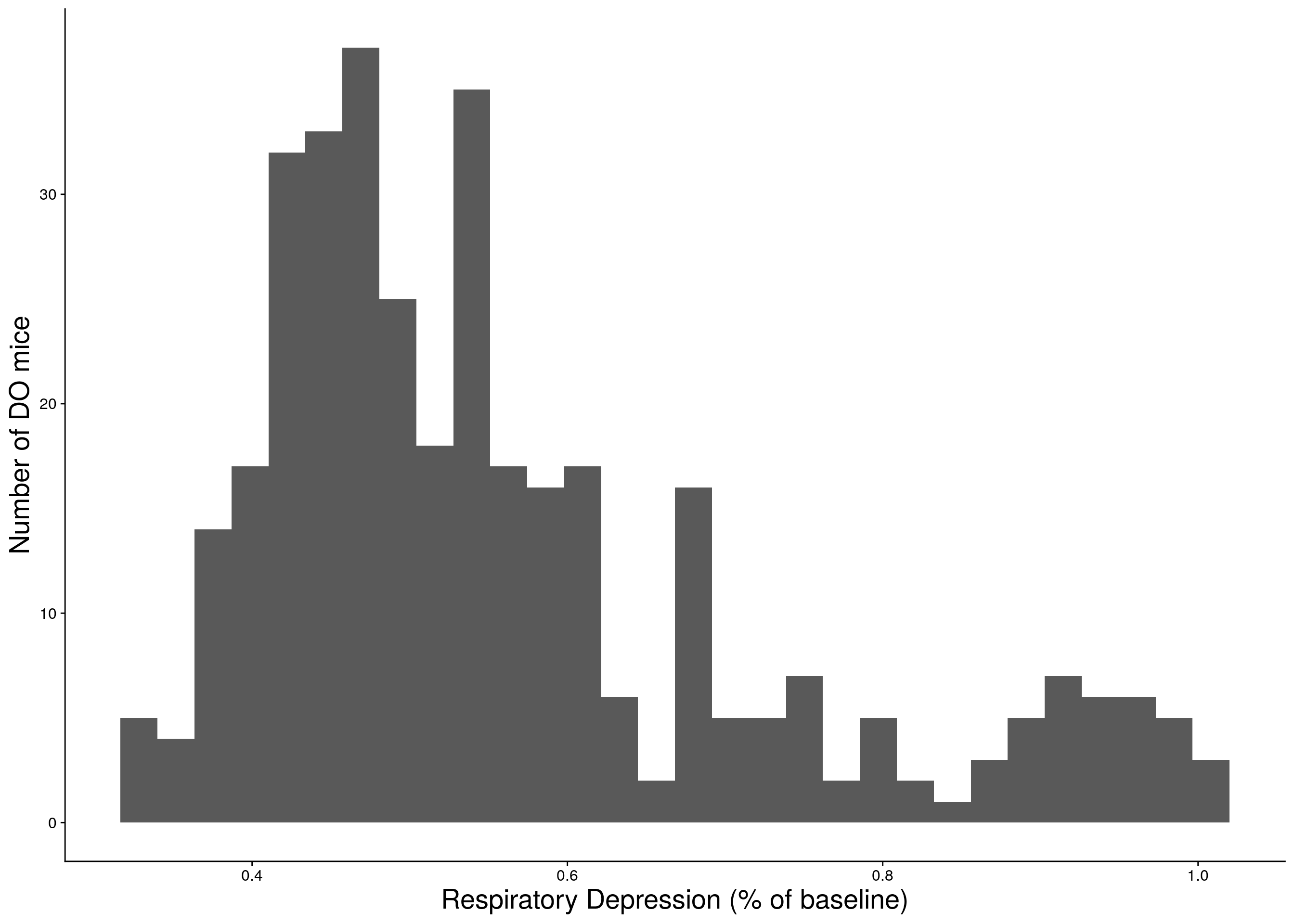
#grid.arrange(a,b,c)

#histgram for other phenotypes
do.pheno %>%
     select(14:35) %>%
     map2(.,.y = colnames(.), ~ ggplot(do.pheno, aes(x = .x)) +
            geom_histogram() +
            xlab(.y) +
            theme(panel.grid.major = element_blank(), panel.grid.minor = element_blank(),
                  panel.background = element_blank(), axis.line = element_line(colour = "black"),
                  text = element_text(size=21))
     ) %>%
     wrap_plots( ncol = 3)
# Warning: Removed 74 rows containing non-finite values (stat_bin).
# Warning: Removed 74 rows containing non-finite values (stat_bin).

# Warning: Removed 74 rows containing non-finite values (stat_bin).

# Warning: Removed 74 rows containing non-finite values (stat_bin).

# Warning: Removed 74 rows containing non-finite values (stat_bin).

# Warning: Removed 74 rows containing non-finite values (stat_bin).

# Warning: Removed 74 rows containing non-finite values (stat_bin).

# Warning: Removed 74 rows containing non-finite values (stat_bin).

# Warning: Removed 74 rows containing non-finite values (stat_bin).

# Warning: Removed 74 rows containing non-finite values (stat_bin).

# Warning: Removed 74 rows containing non-finite values (stat_bin).

# Warning: Removed 74 rows containing non-finite values (stat_bin).

# Warning: Removed 74 rows containing non-finite values (stat_bin).

# Warning: Removed 74 rows containing non-finite values (stat_bin).
# Warning: Removed 75 rows containing non-finite values (stat_bin).
# Warning: Removed 74 rows containing non-finite values (stat_bin).

# Warning: Removed 74 rows containing non-finite values (stat_bin).

# Warning: Removed 74 rows containing non-finite values (stat_bin).

# Warning: Removed 74 rows containing non-finite values (stat_bin).

# Warning: Removed 74 rows containing non-finite values (stat_bin).

# Warning: Removed 74 rows containing non-finite values (stat_bin).

# Warning: Removed 74 rows containing non-finite values (stat_bin).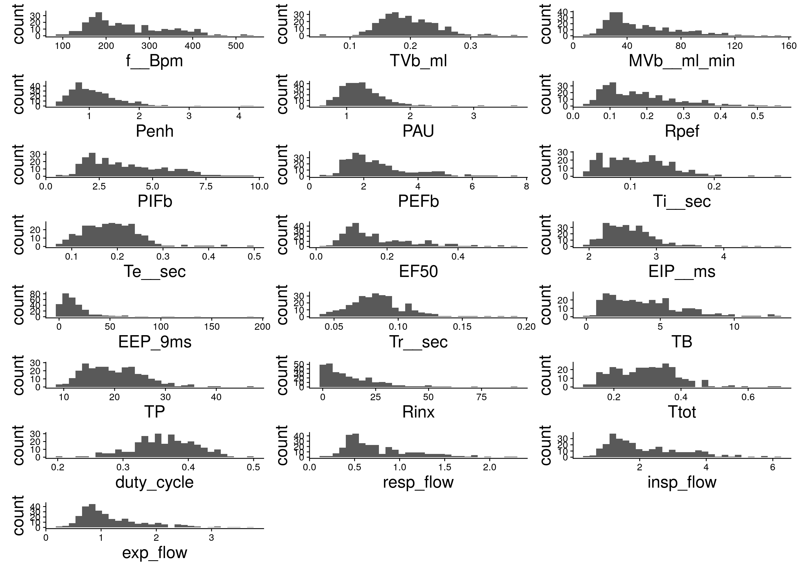
#boxplot on the rankz data------------
#survival time
surv <- do.pheno[,c(2,3,10)]
surv <- surv[complete.cases(surv), ]
p1 <- ggplot(surv, aes(x=Sex, y=rz.transform(Survival.Time), group = Sex, fill = Sex, alpha = 0.9)) +
  geom_boxplot(show.legend = F , outlier.size = 1.5, notchwidth = 0.85) +
  geom_jitter(color="black", size=0.8, alpha=0.9) +
  scale_fill_brewer(palette="Blues") +
  ylab("Survival Time") +
  xlab("Sex") +
  labs(fill = "") +
  theme(legend.position = "none",
        panel.grid.major = element_blank(),
        panel.grid.minor = element_blank(),
        panel.background = element_blank(),
        axis.line = element_line(colour = "black"),
        text = element_text(size=21),
        axis.title=element_text(size=21)) +
  guides(shape = guide_legend(override.aes = list(size = 12)))
p1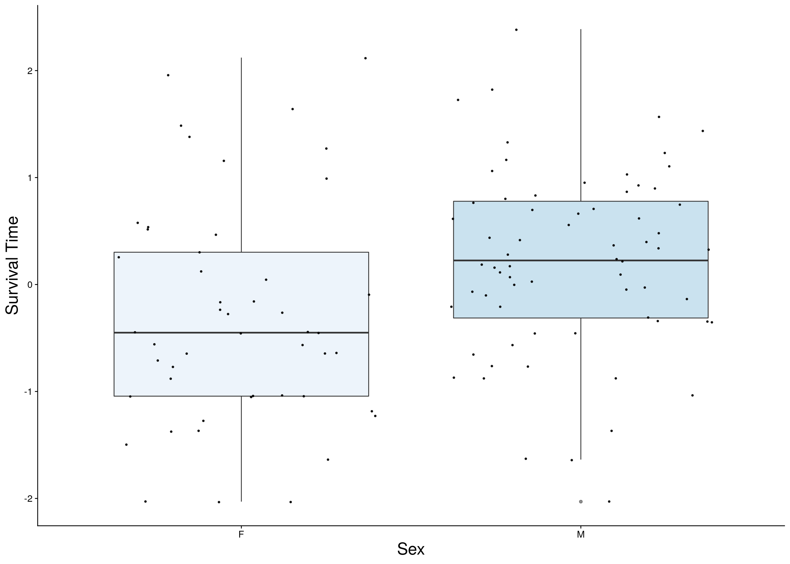
reco <- do.pheno[,c(2,3,11)]
reco <- reco[complete.cases(reco), ]
p2 <- ggplot(reco, aes(x=Sex, y=rz.transform(Recovery.Time), group = Sex, fill = Sex, alpha = 0.9)) +
  geom_boxplot(show.legend = F , outlier.size = 1.5, notchwidth = 0.85) +
  geom_jitter(color="black", size=0.8, alpha=0.9) +
  scale_fill_brewer(palette="Blues") +
  ylab("Recovery Time") +
  xlab("Sex") +
  labs(fill = "") +
  theme(legend.position = "none",
        panel.grid.major = element_blank(),
        panel.grid.minor = element_blank(),
        panel.background = element_blank(),
        axis.line = element_line(colour = "black"),
        text = element_text(size=21),
        axis.title=element_text(size=21)) +
  guides(shape = guide_legend(override.aes = list(size = 12)))
p2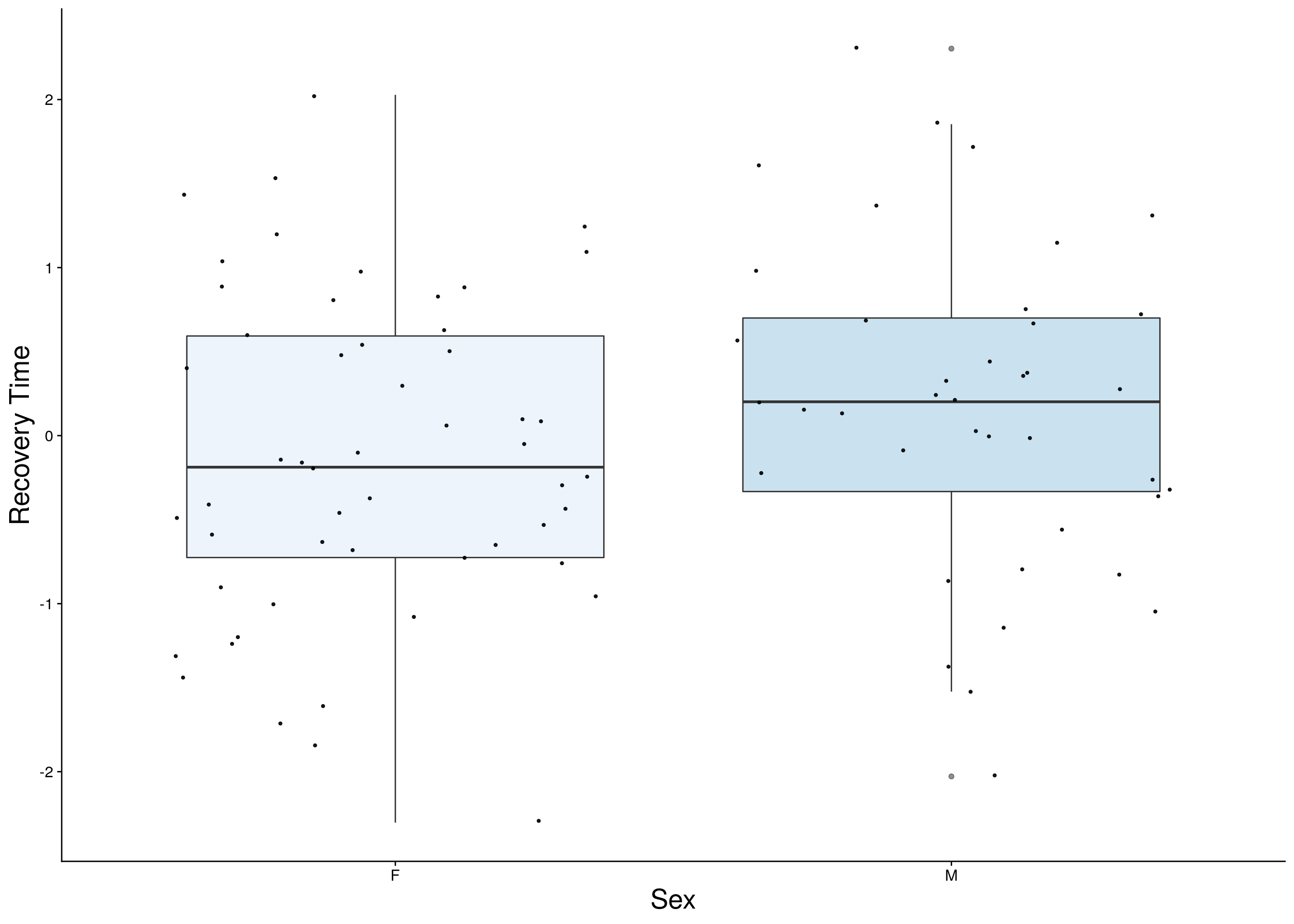
dep <- do.pheno[,c(2,3,9)]
dep <- dep[complete.cases(dep), ]
p3 <- ggplot(dep, aes(x=Sex, y=rz.transform(Min.depression), group = Sex, fill = Sex, alpha = 0.9)) +
  geom_boxplot(show.legend = F , outlier.size = 1.5, notchwidth = 0.85) +
  geom_jitter(color="black", size=0.8, alpha=0.9) +
  scale_fill_brewer(palette="Blues") +
  ylab("Min depression") +
  xlab("Sex") +
  labs(fill = "") +
  theme(legend.position = "none",
        panel.grid.major = element_blank(),
        panel.grid.minor = element_blank(),
        panel.background = element_blank(),
        axis.line = element_line(colour = "black"),
        text = element_text(size=21),
        axis.title=element_text(size=21)) +
  guides(shape = guide_legend(override.aes = list(size = 12)))
p3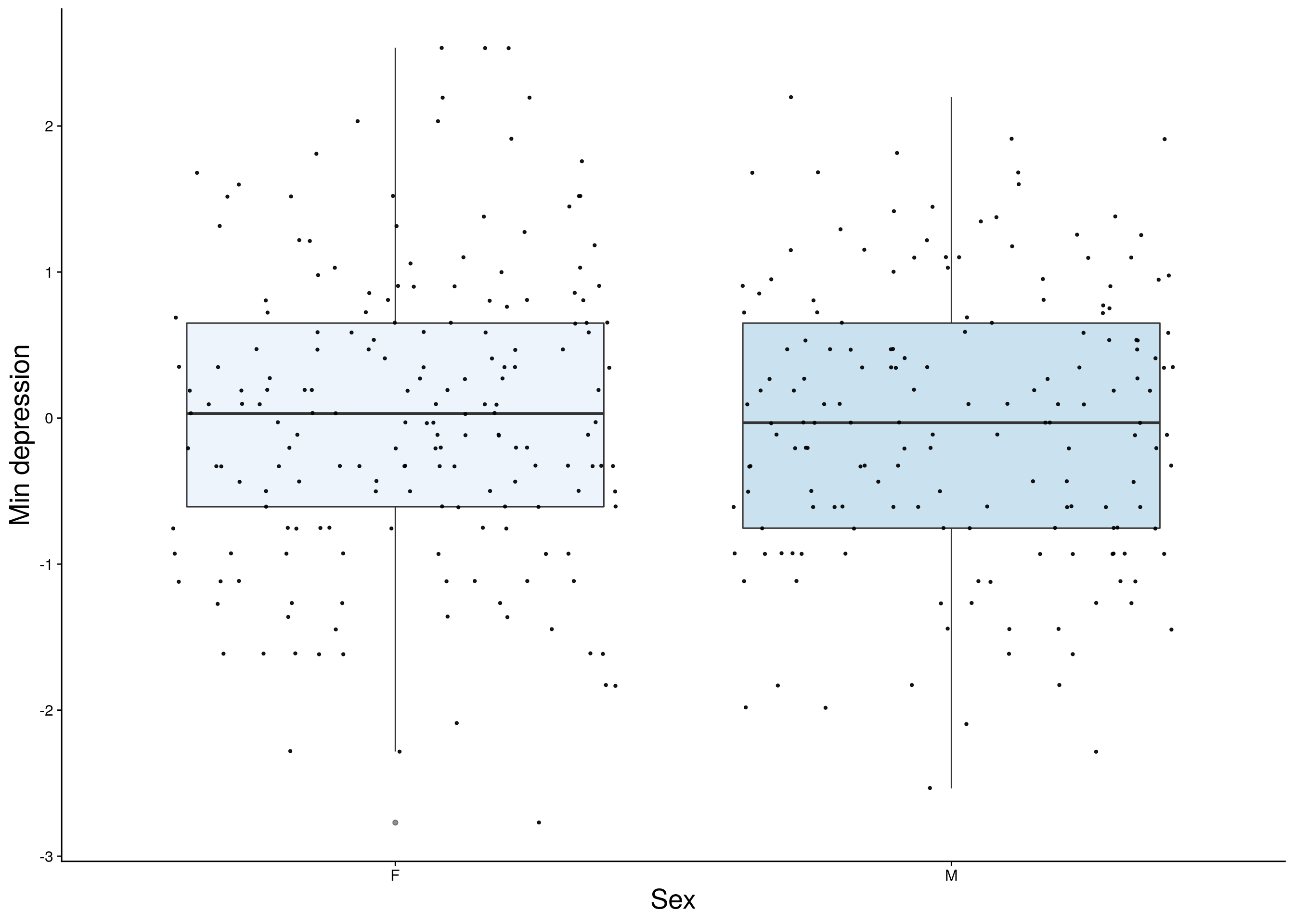
#histogram
a <- ggplot(data=do.pheno, aes(rz.transform(Survival.Time))) +
  geom_histogram() +
  ylab("Number of DO mice") + xlab("RankZ of Survival Time (h)") +
  theme(panel.grid.major = element_blank(), panel.grid.minor = element_blank(),
        panel.background = element_blank(), axis.line = element_line(colour = "black"),
        text = element_text(size=21))
print(a)
# Warning: Removed 251 rows containing non-finite values (stat_bin).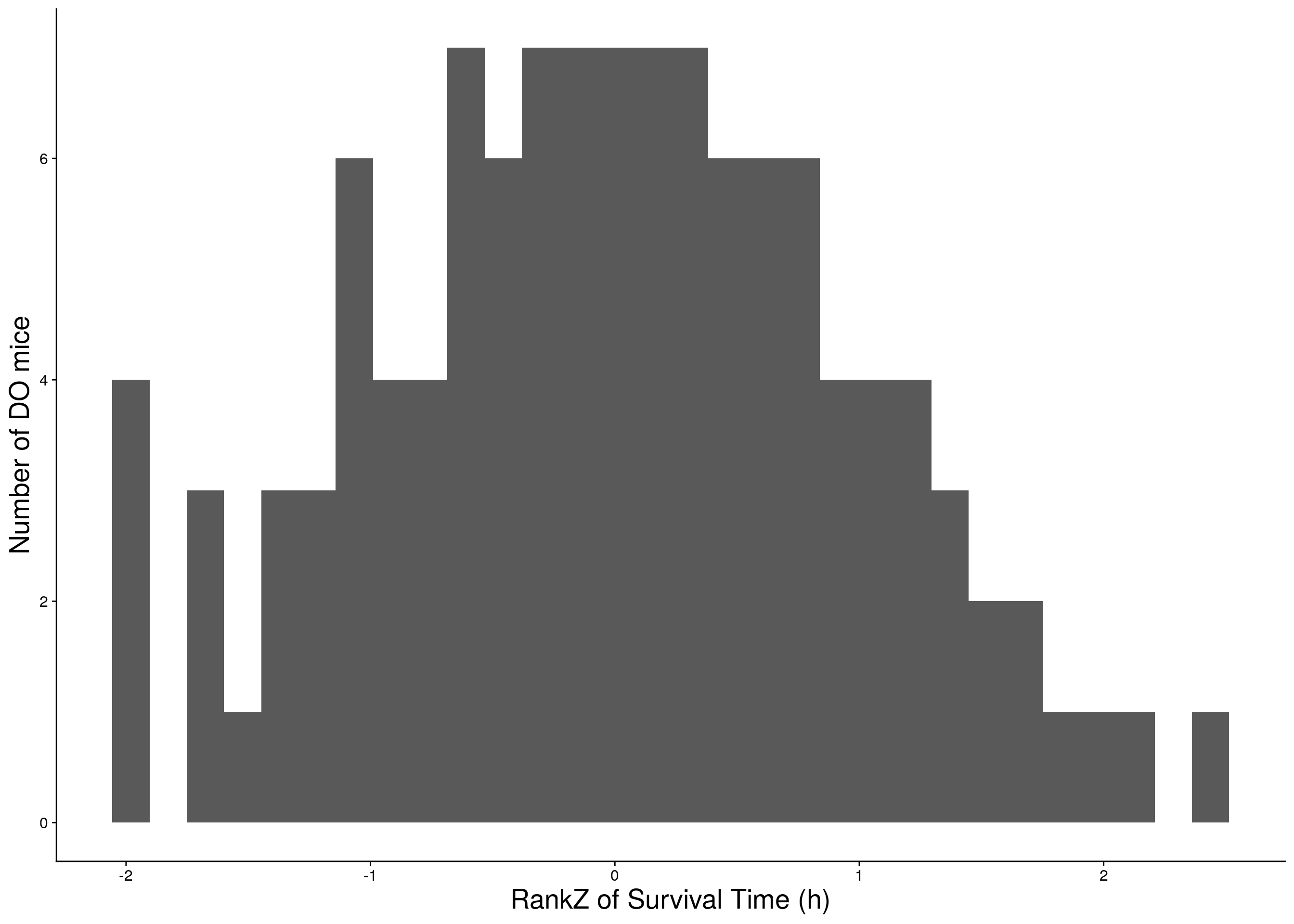
| Version | Author | Date |
|---|---|---|
| fd4dc88 | xhyuo | 2023-01-11 |
b <- ggplot(data=do.pheno, aes(rz.transform(Recovery.Time))) +
  geom_histogram() +
  ylab("Number of DO mice") + xlab("RankZ of Recovery Time (h)") +
  theme(panel.grid.major = element_blank(), panel.grid.minor = element_blank(),
        panel.background = element_blank(), axis.line = element_line(colour = "black"),
        text = element_text(size=21))
print(b)
# Warning: Removed 275 rows containing non-finite values (stat_bin).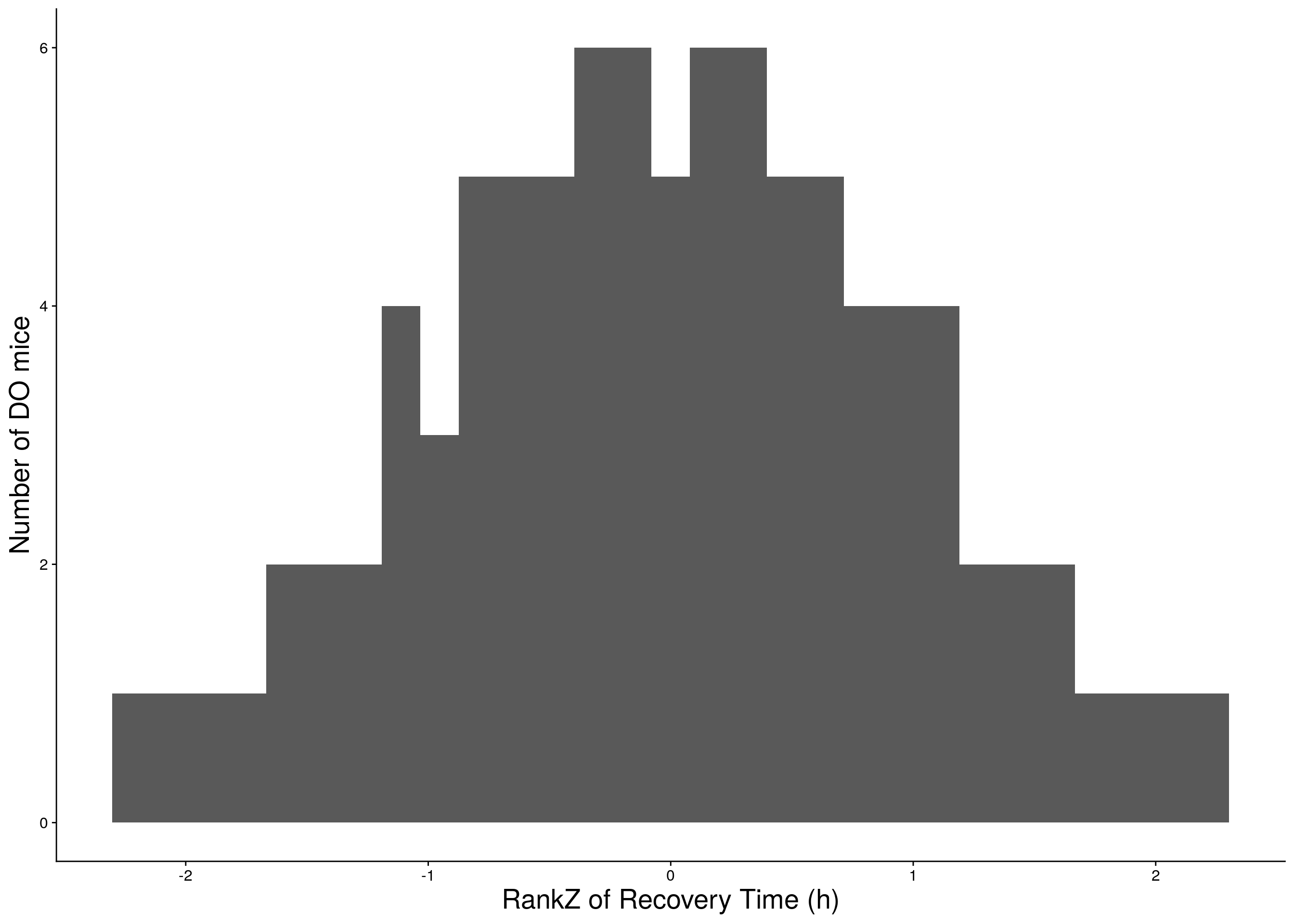
| Version | Author | Date |
|---|---|---|
| fd4dc88 | xhyuo | 2023-01-11 |
c <- ggplot(data=do.pheno, aes(rz.transform(Min.depression))) +
  geom_histogram() +
  ylab("Number of DO mice") + xlab("RankZ of Respiratory Depression (% of baseline)") +
  theme(panel.grid.major = element_blank(), panel.grid.minor = element_blank(),
        panel.background = element_blank(), axis.line = element_line(colour = "black"),
        text = element_text(size=21))
print(c)
# Warning: Removed 12 rows containing non-finite values (stat_bin).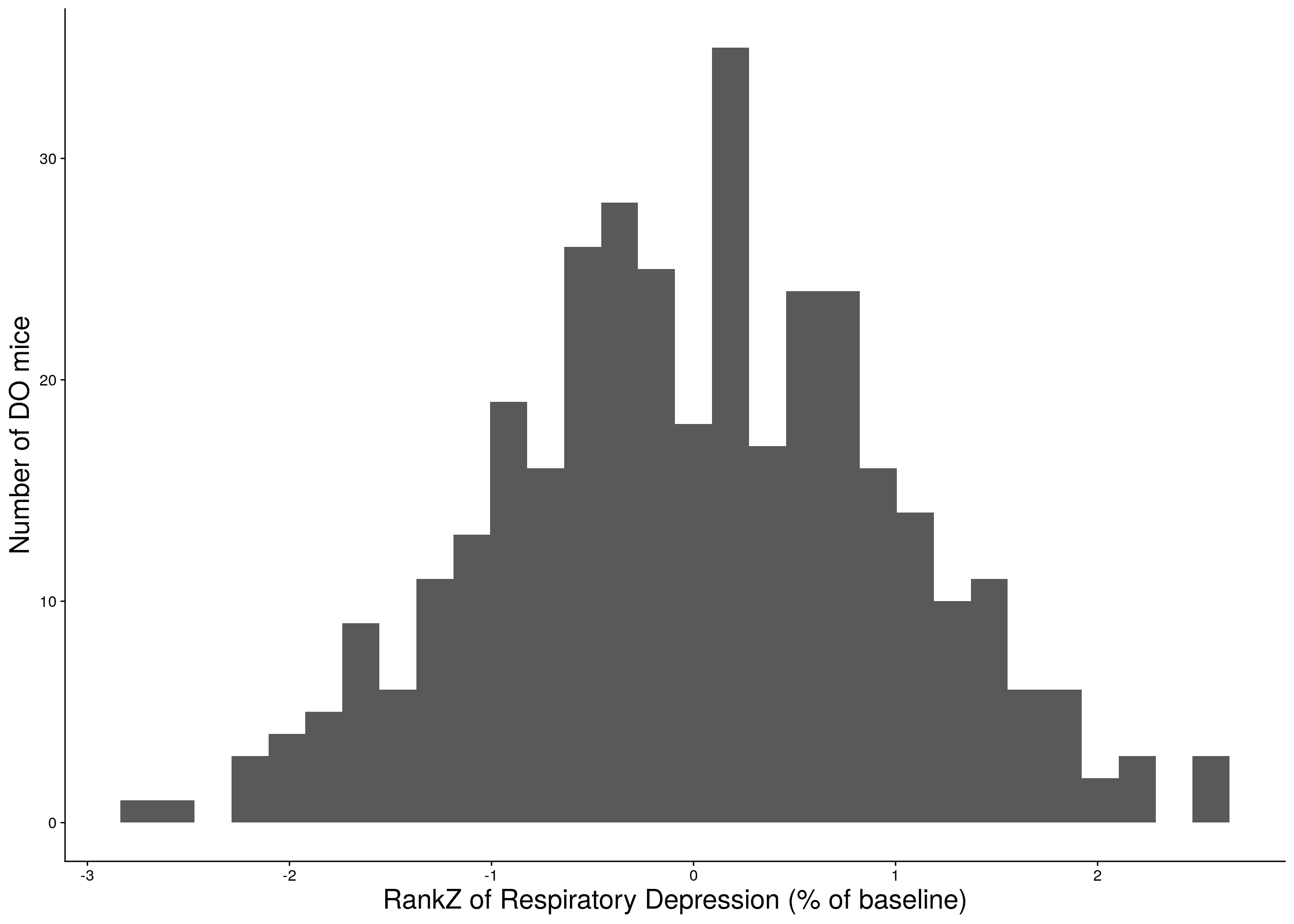
| Version | Author | Date |
|---|---|---|
| fd4dc88 | xhyuo | 2023-01-11 |
#grid.arrange(a,b,c)

#histgram for other phenotypes
do.pheno %>%
     select(14:35) %>%
     map2(.,.y = colnames(.), ~ ggplot(do.pheno, aes(x = rz.transform(.x))) +
               geom_histogram() +
               xlab(.y)
     ) %>%
     wrap_plots( ncol = 3)
# Warning: Removed 74 rows containing non-finite values (stat_bin).

# Warning: Removed 74 rows containing non-finite values (stat_bin).

# Warning: Removed 74 rows containing non-finite values (stat_bin).

# Warning: Removed 74 rows containing non-finite values (stat_bin).

# Warning: Removed 74 rows containing non-finite values (stat_bin).

# Warning: Removed 74 rows containing non-finite values (stat_bin).

# Warning: Removed 74 rows containing non-finite values (stat_bin).

# Warning: Removed 74 rows containing non-finite values (stat_bin).

# Warning: Removed 74 rows containing non-finite values (stat_bin).

# Warning: Removed 74 rows containing non-finite values (stat_bin).

# Warning: Removed 74 rows containing non-finite values (stat_bin).

# Warning: Removed 74 rows containing non-finite values (stat_bin).

# Warning: Removed 74 rows containing non-finite values (stat_bin).

# Warning: Removed 74 rows containing non-finite values (stat_bin).
# Warning: Removed 75 rows containing non-finite values (stat_bin).
# Warning: Removed 74 rows containing non-finite values (stat_bin).

# Warning: Removed 74 rows containing non-finite values (stat_bin).

# Warning: Removed 74 rows containing non-finite values (stat_bin).

# Warning: Removed 74 rows containing non-finite values (stat_bin).

# Warning: Removed 74 rows containing non-finite values (stat_bin).

# Warning: Removed 74 rows containing non-finite values (stat_bin).

# Warning: Removed 74 rows containing non-finite values (stat_bin).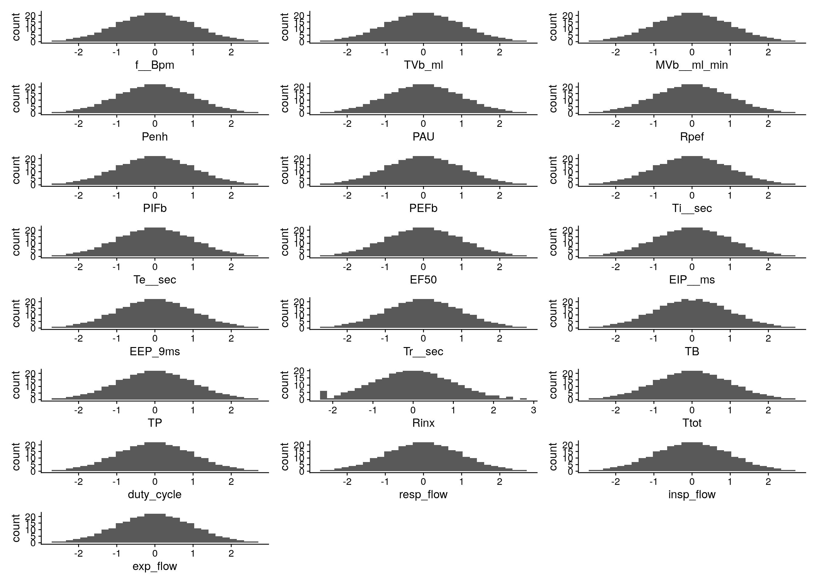
| Version | Author | Date |
|---|---|---|
| fd4dc88 | xhyuo | 2023-01-11 |
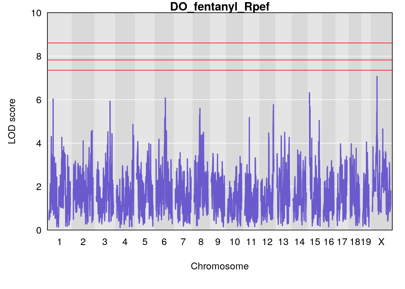
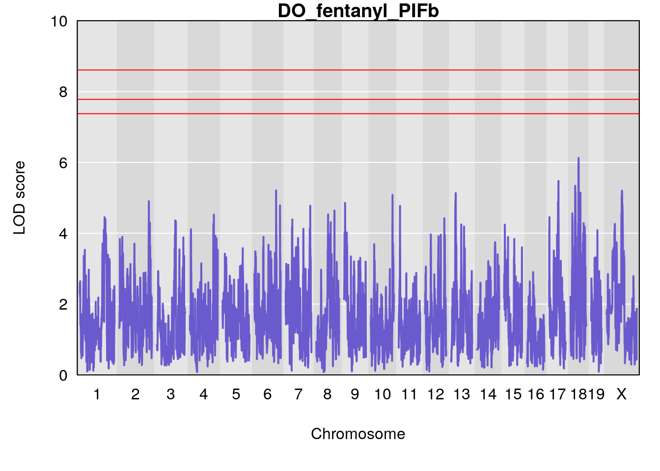
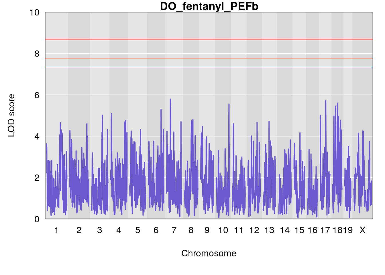
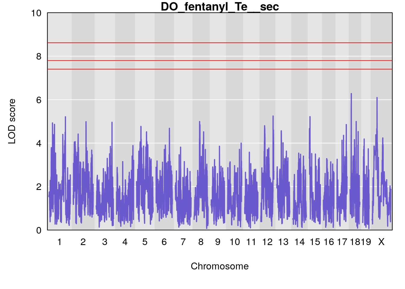
Plot qtl mapping on array
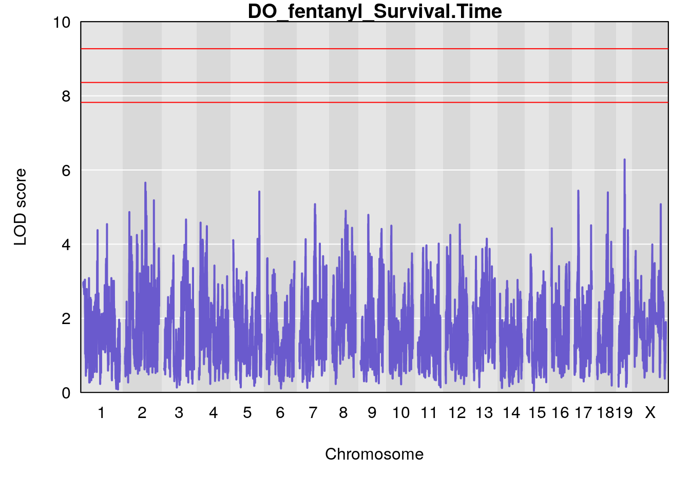
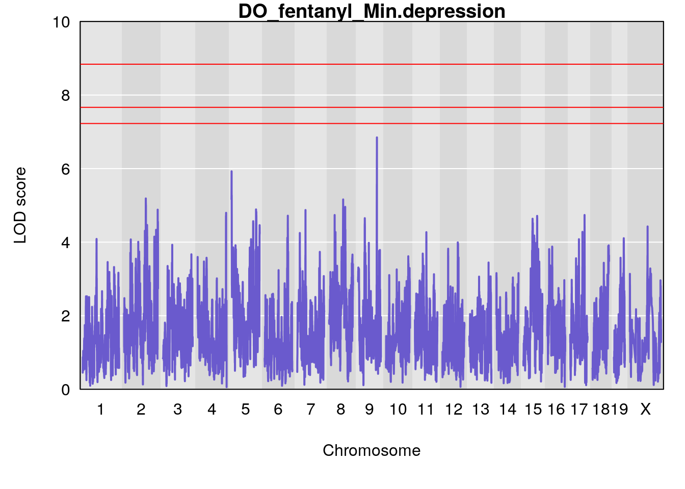
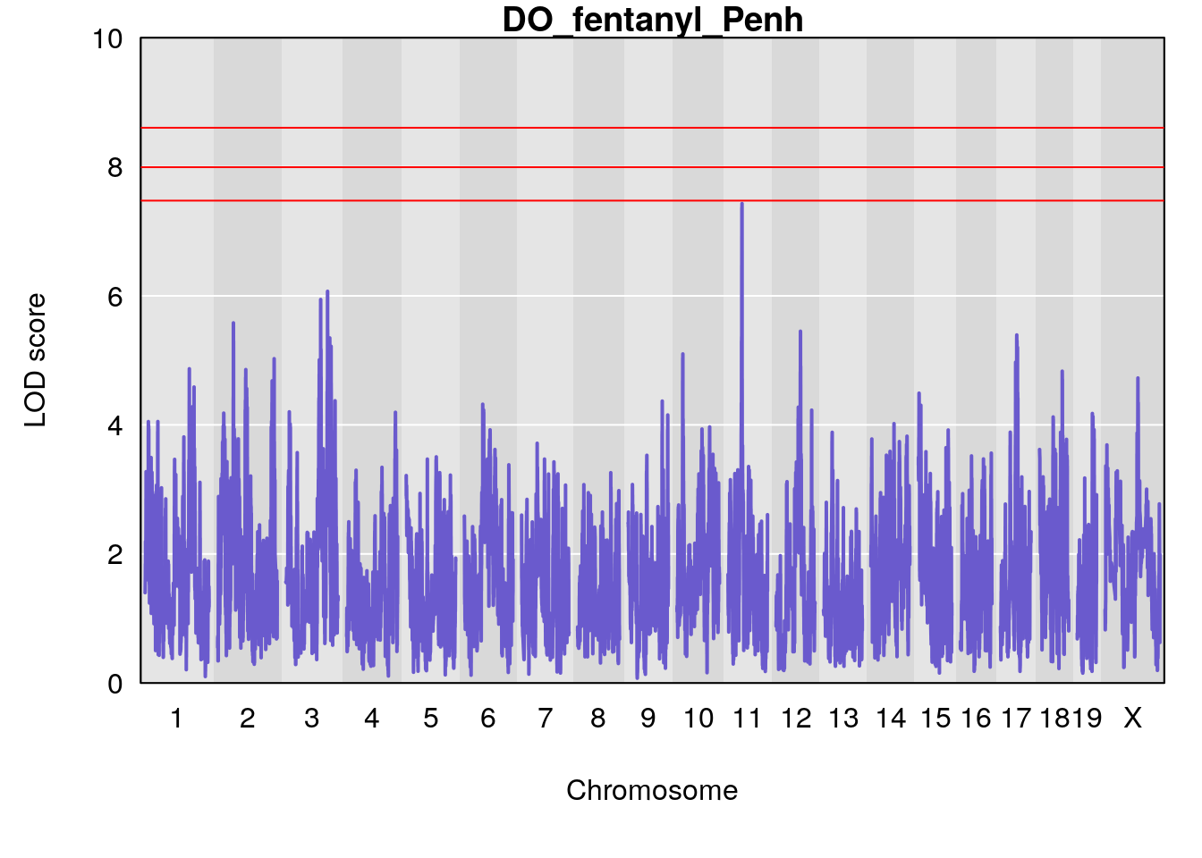
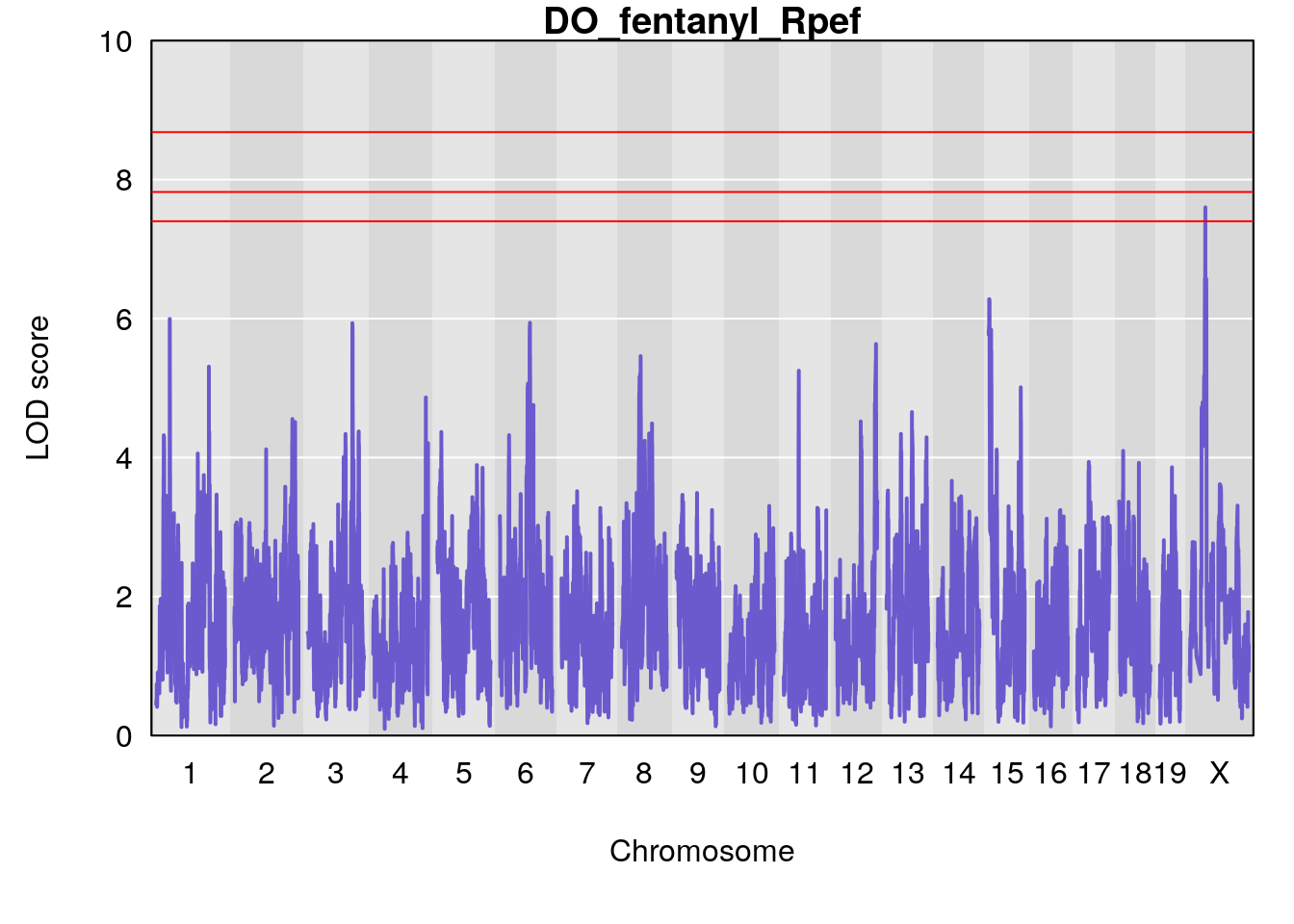
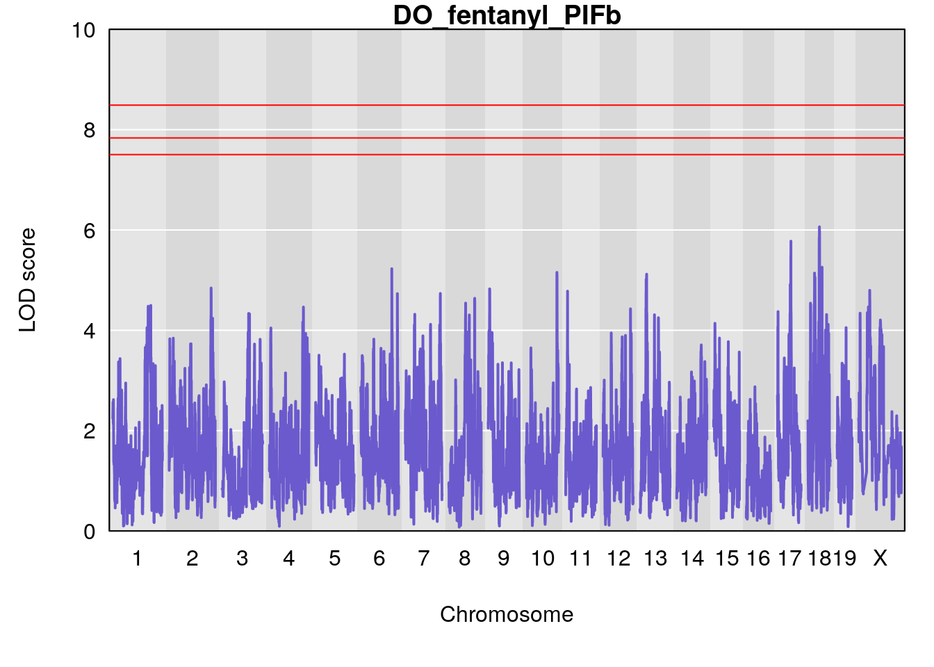
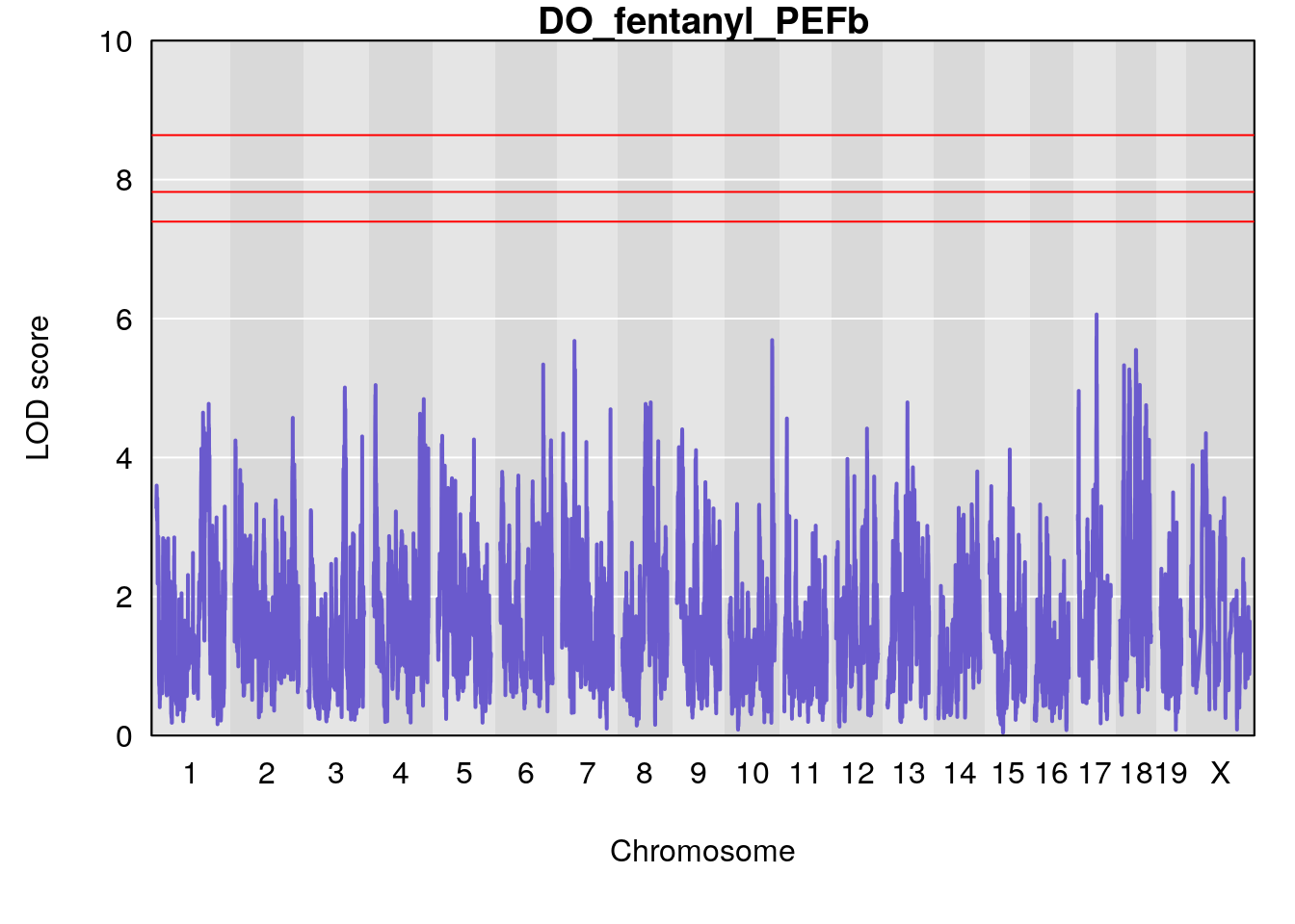
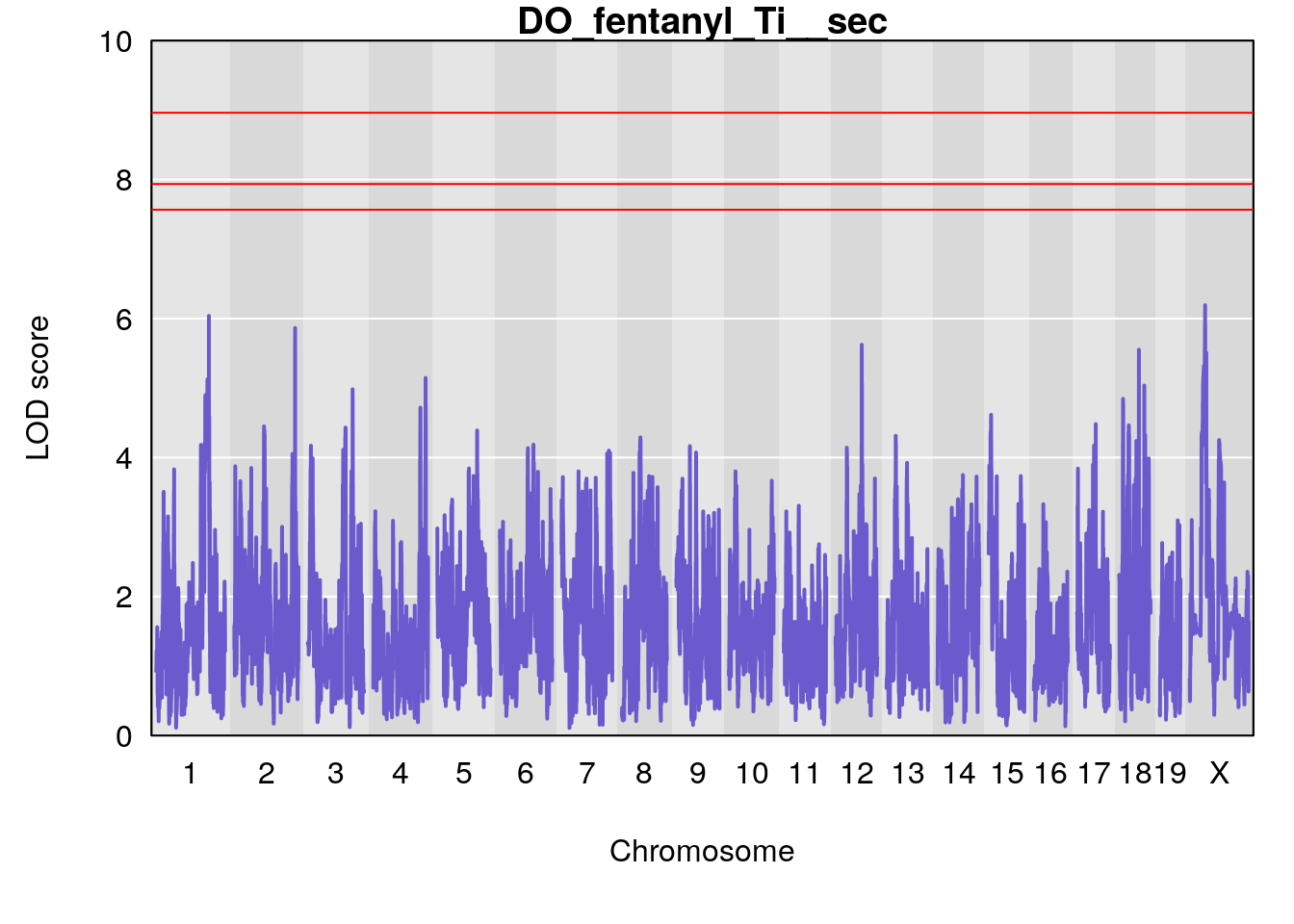
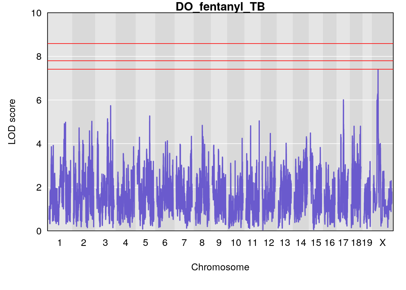
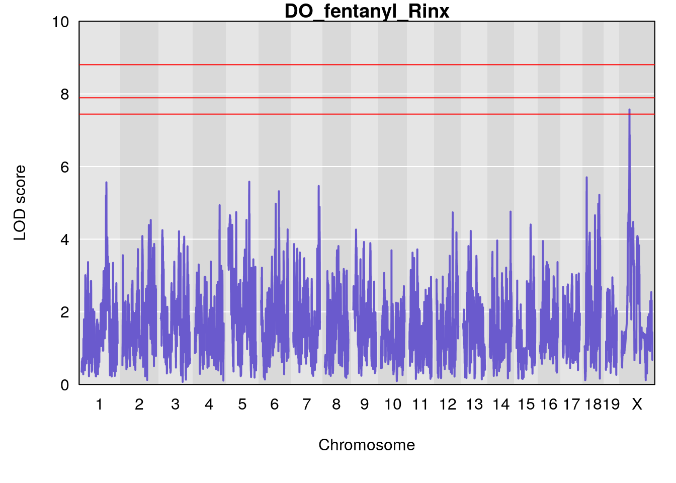
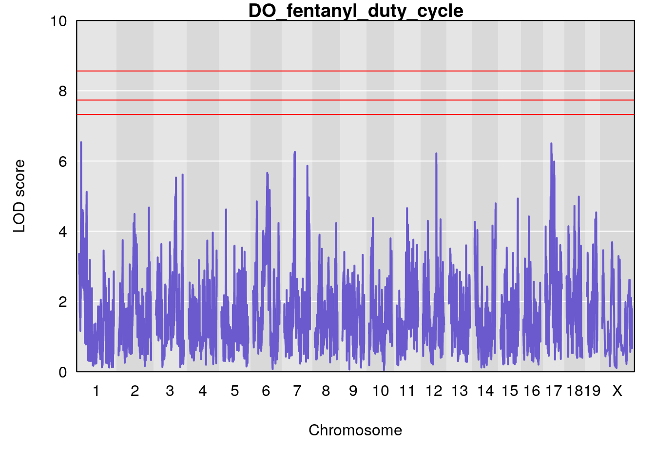
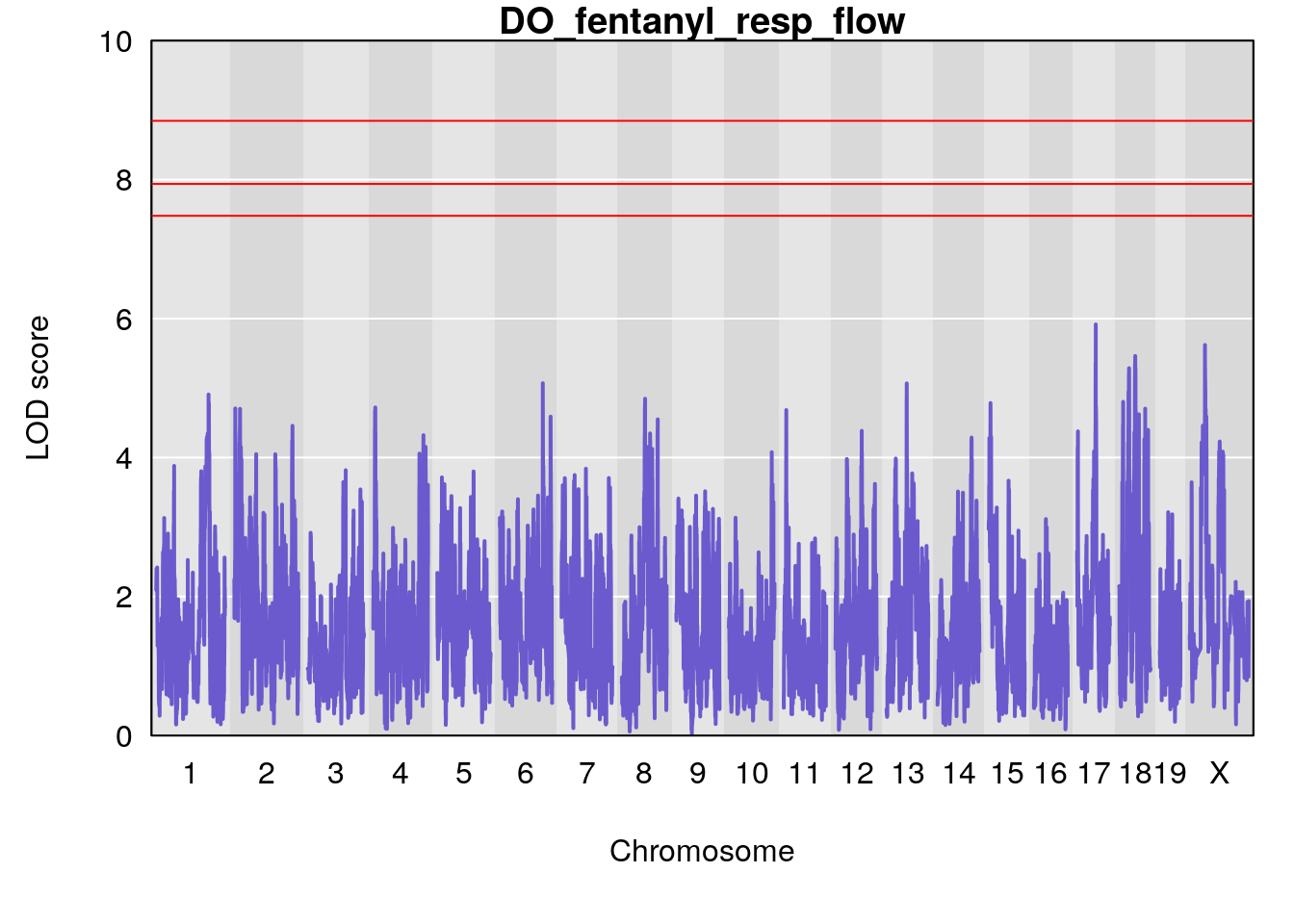
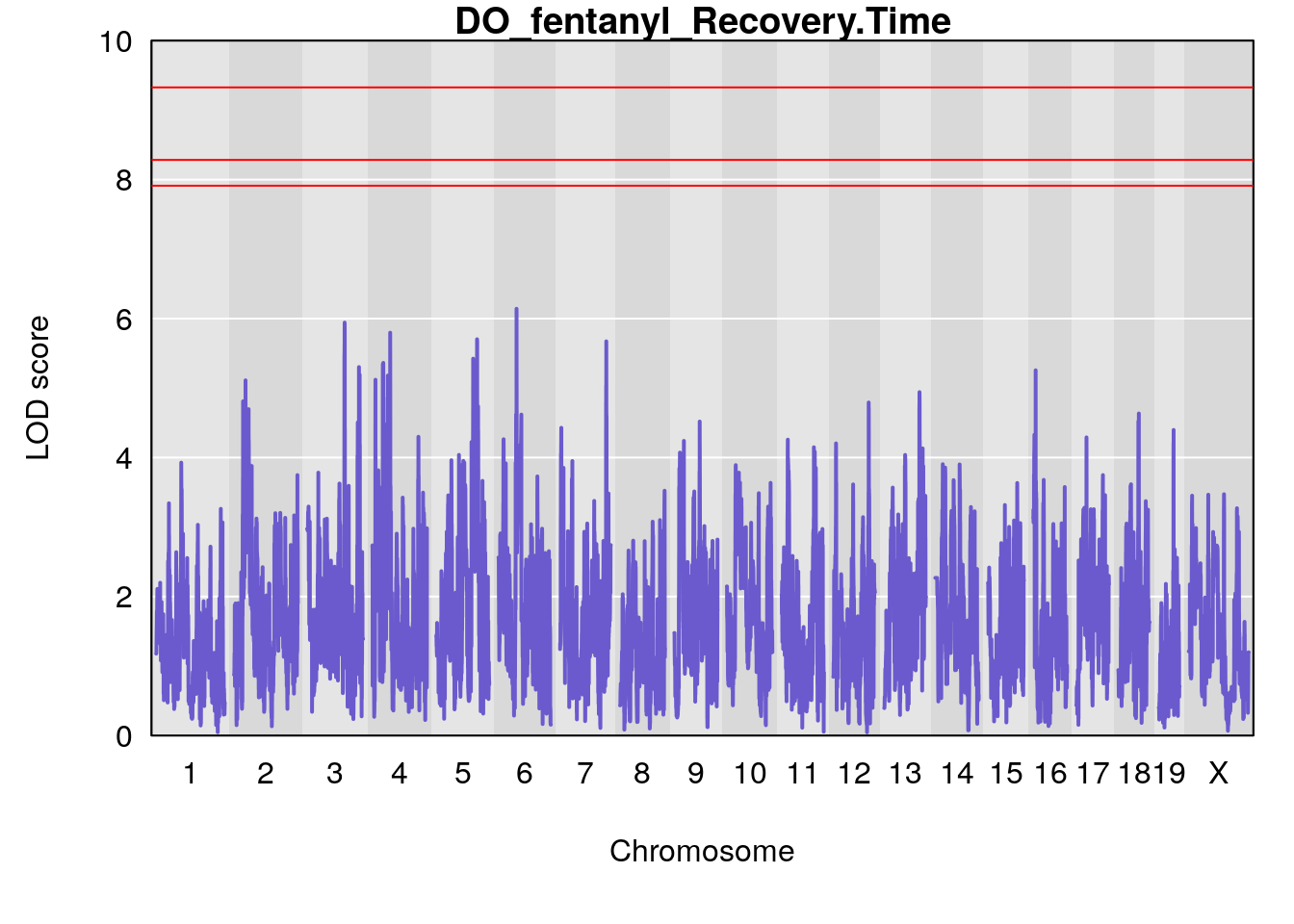
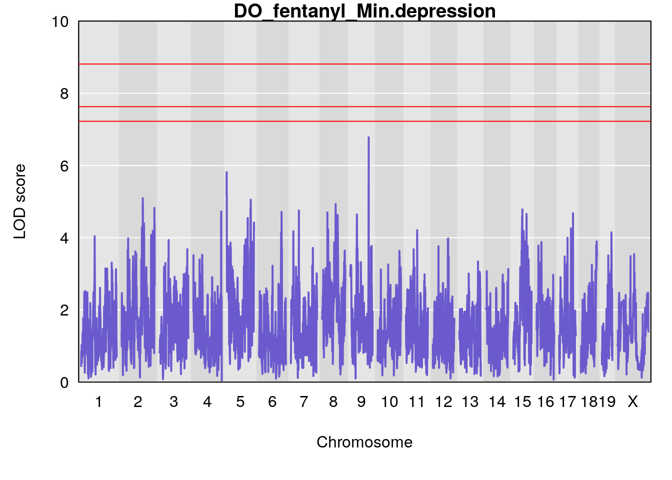
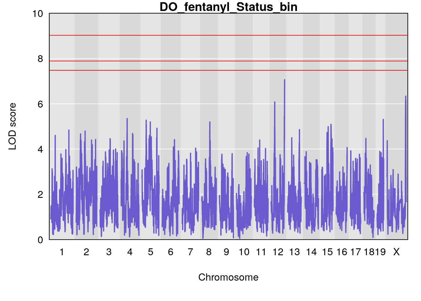
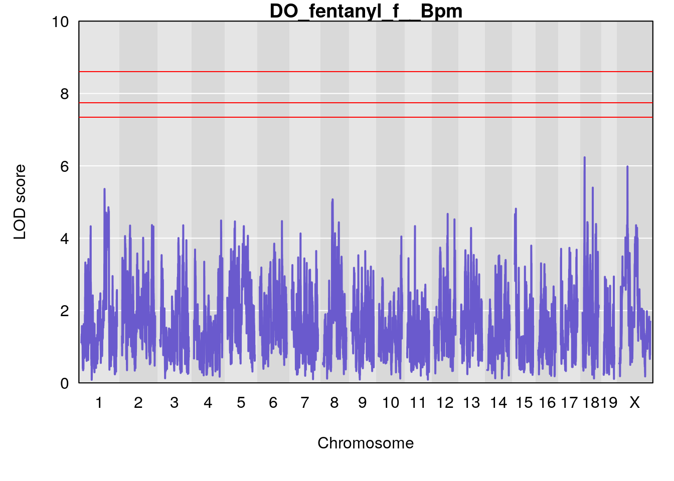
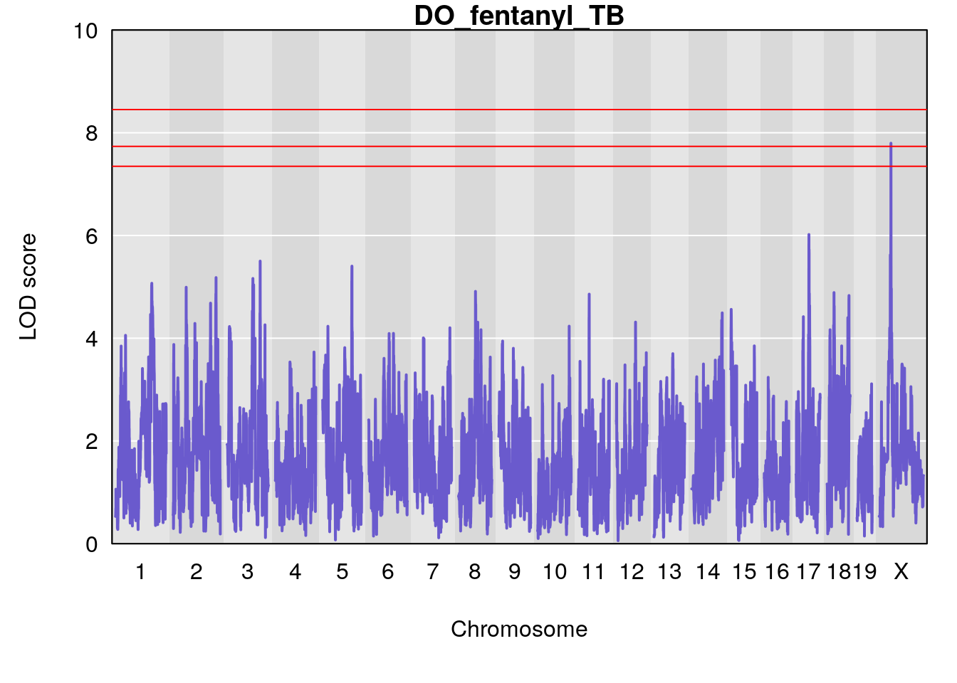
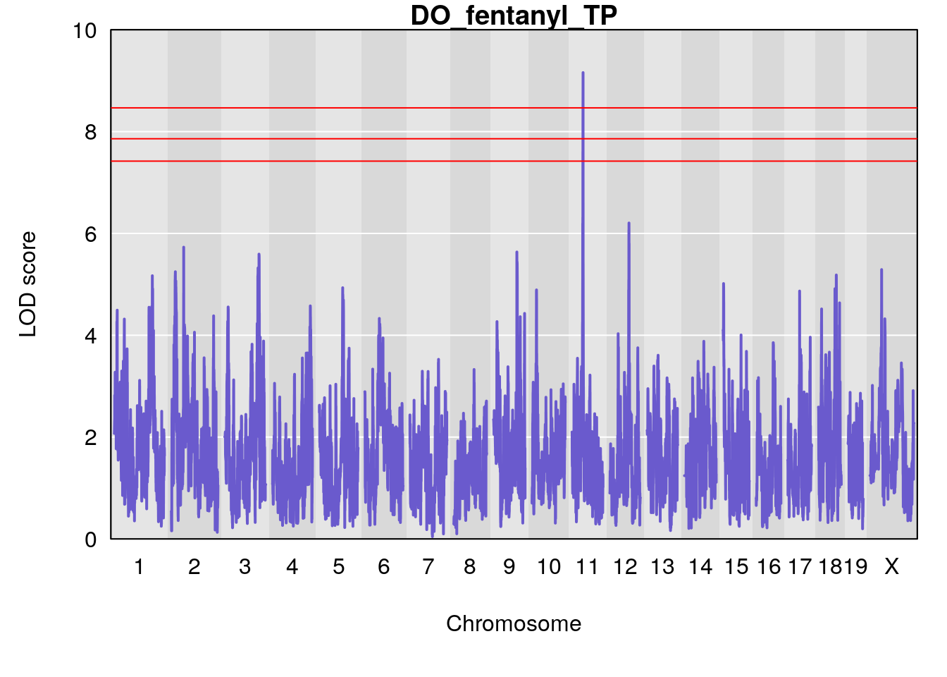
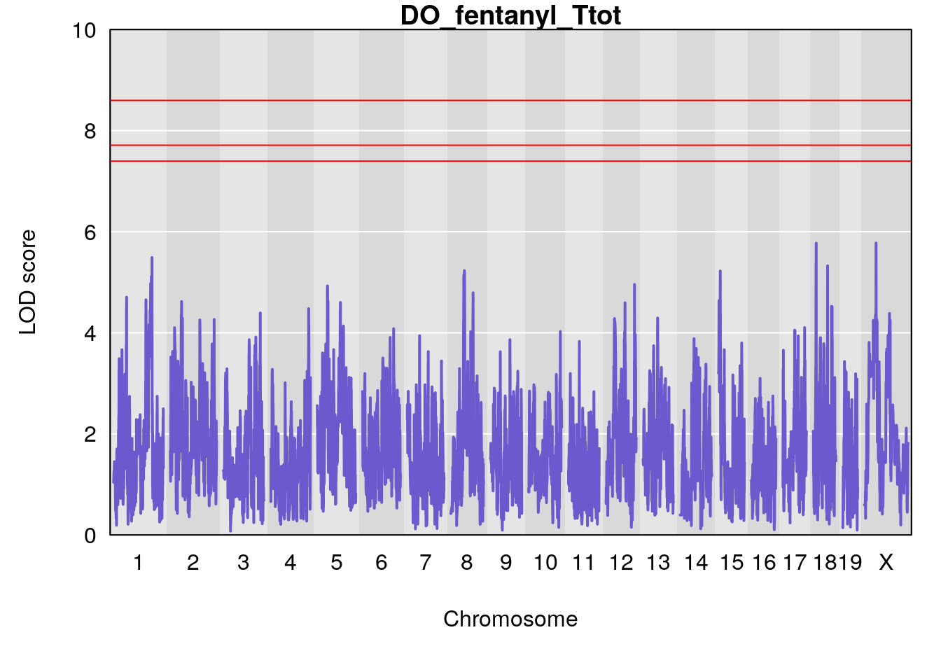
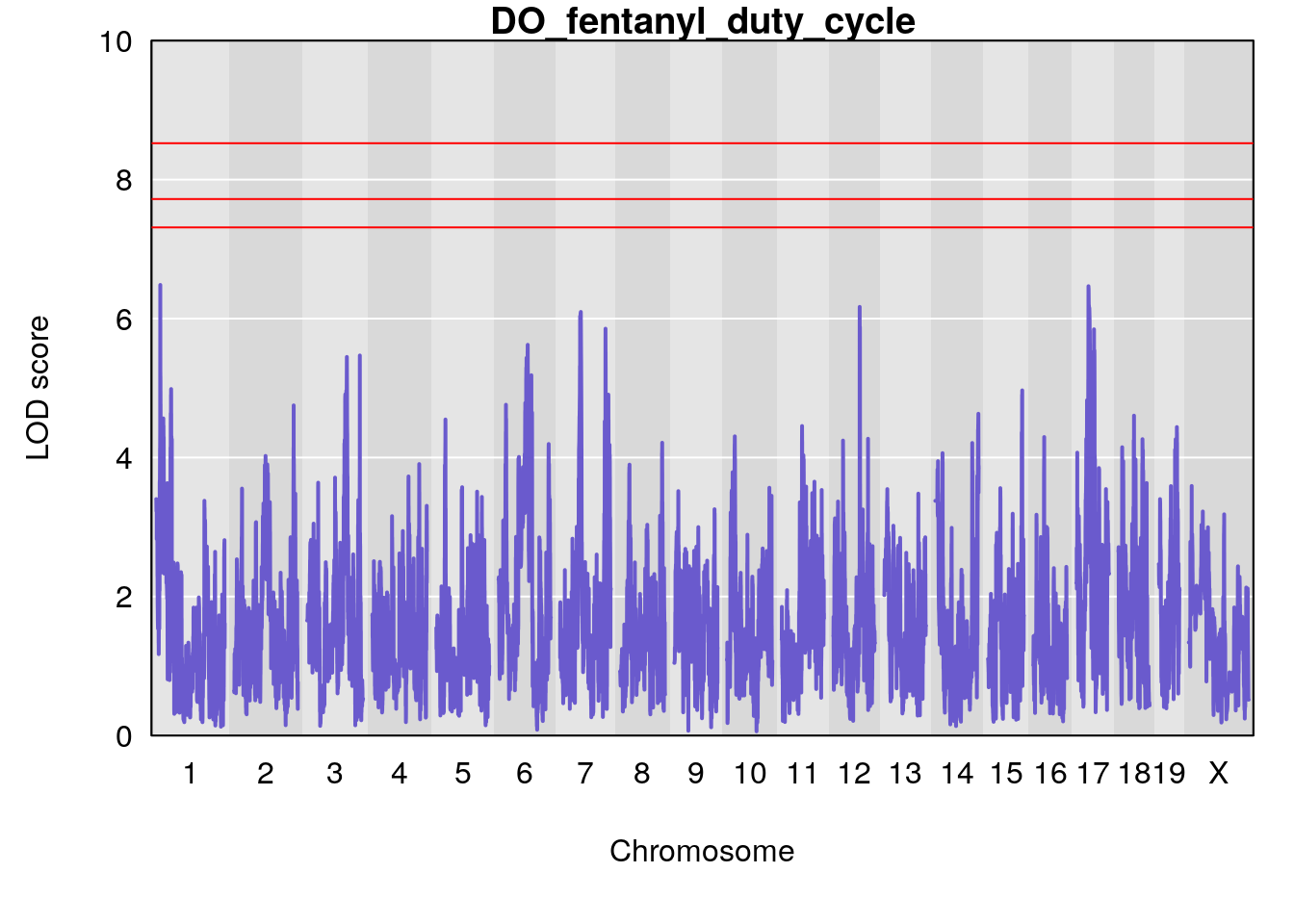
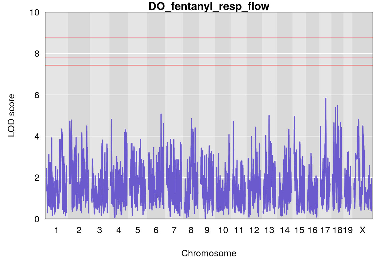
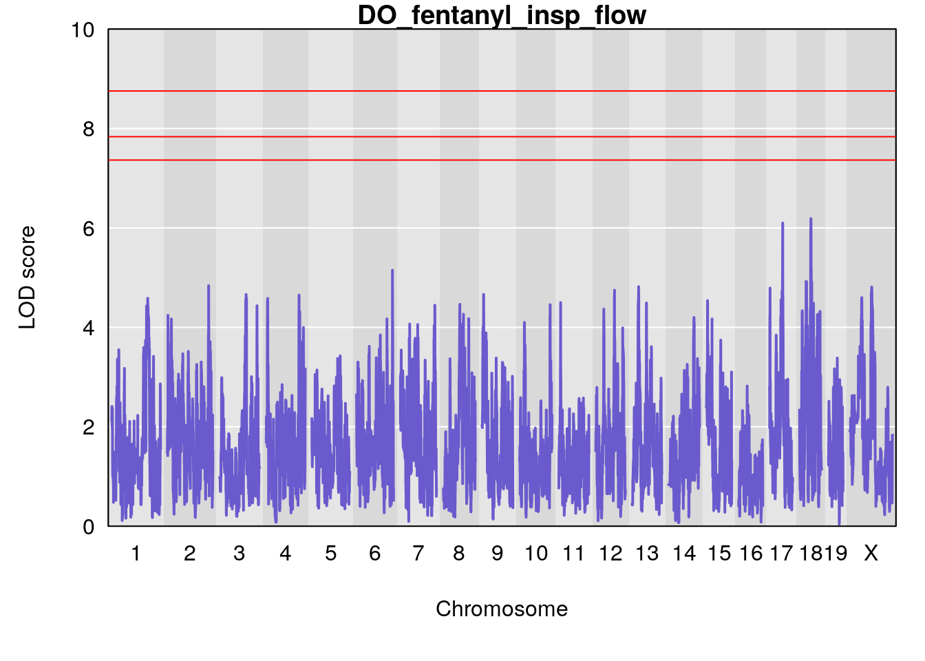
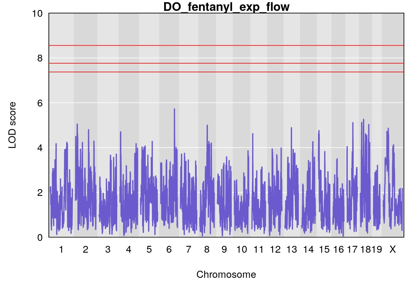
load("output/Fentanyl/qtl.fentanyl.out.RData")
#genome-wide plot
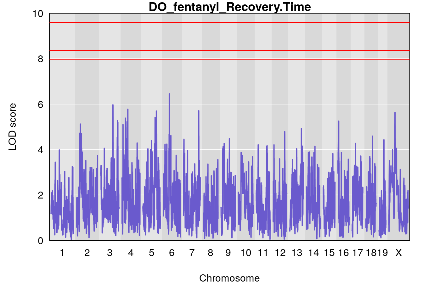
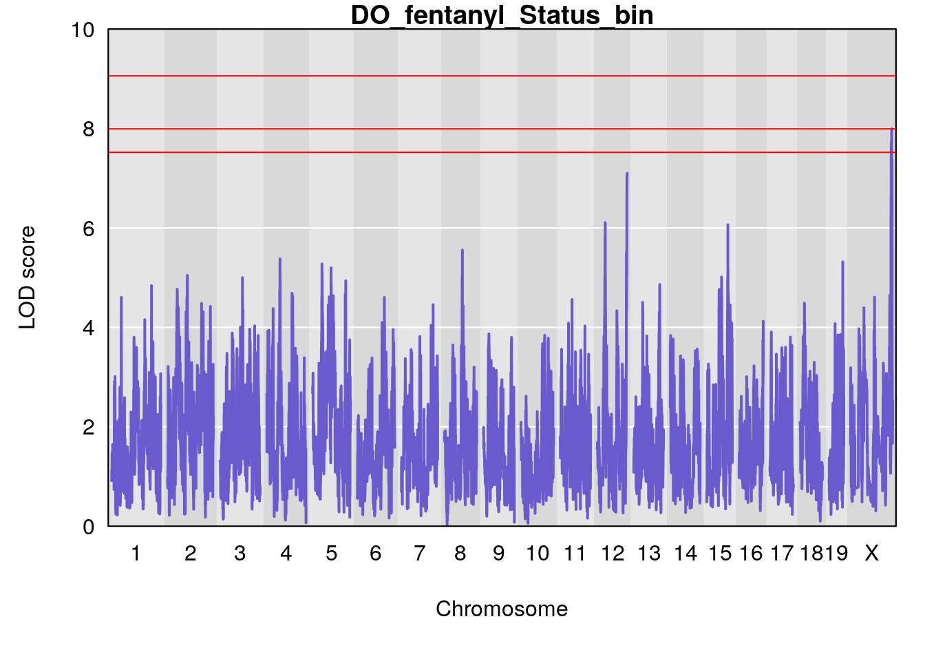
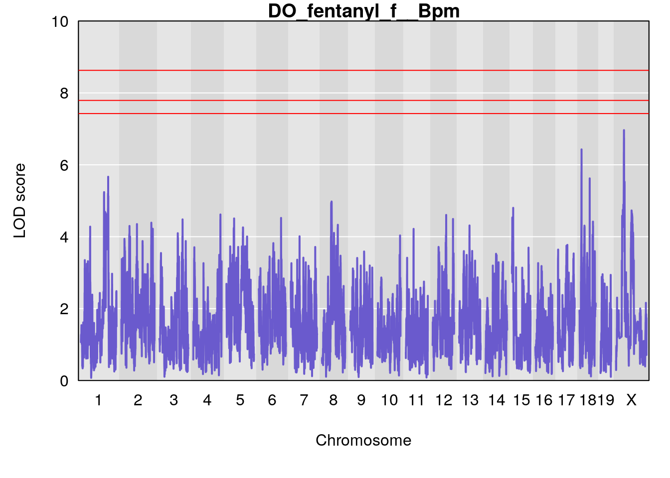
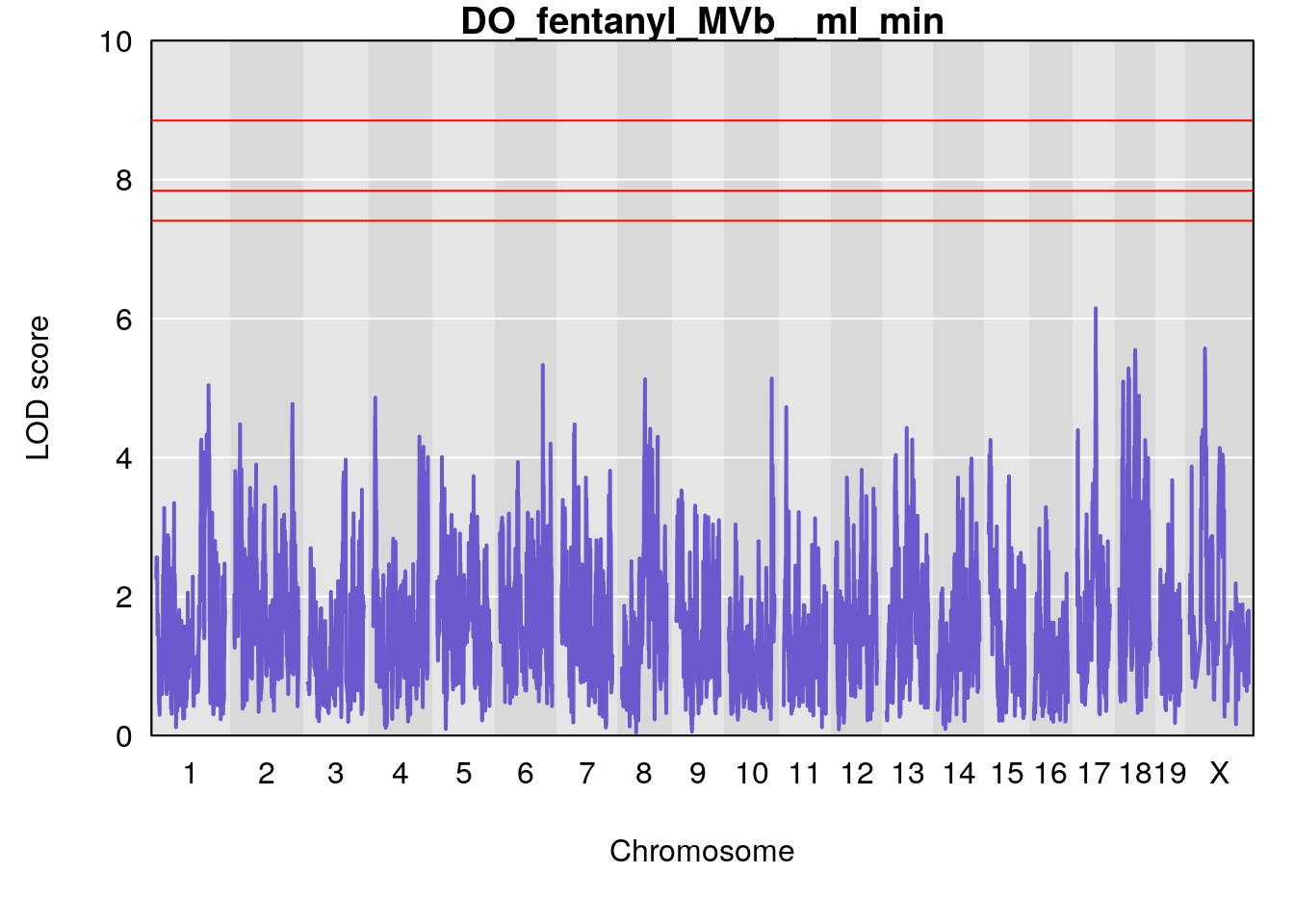
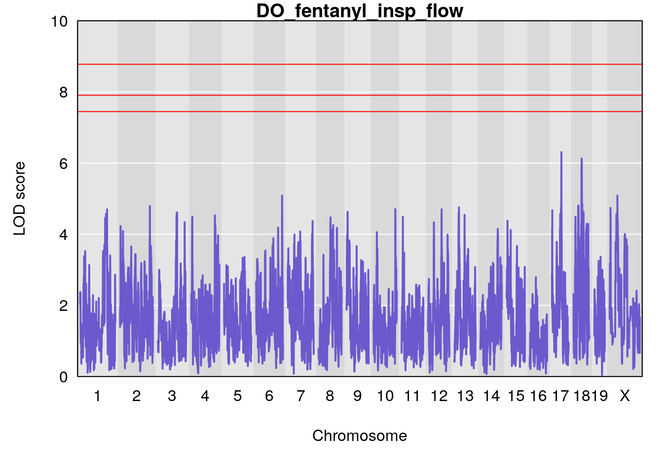
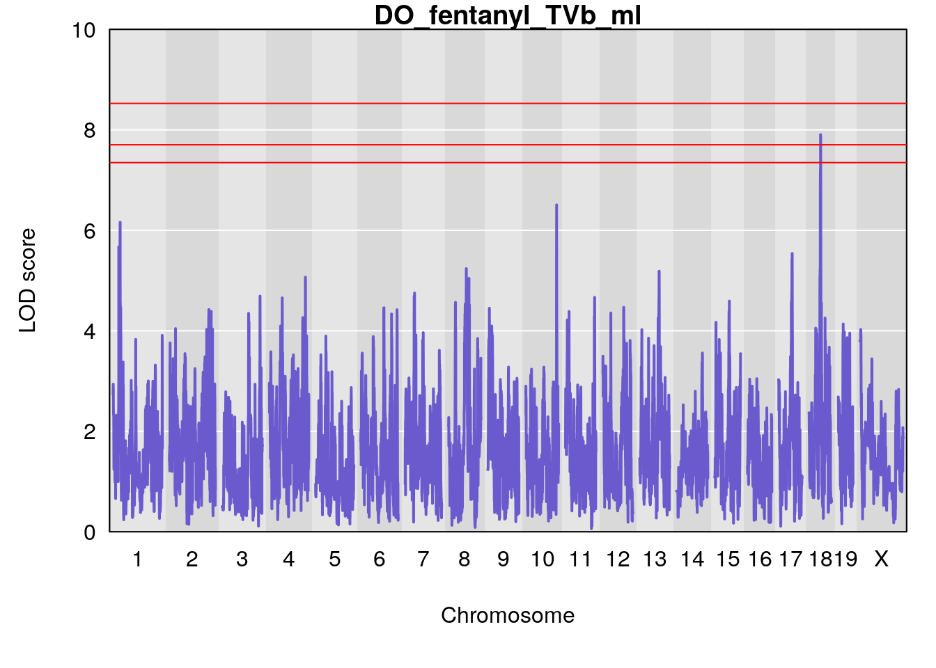
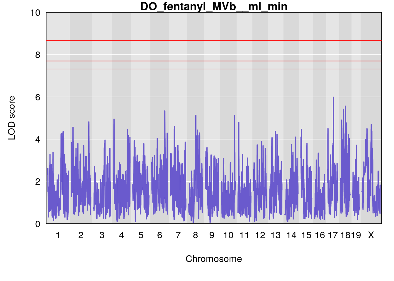
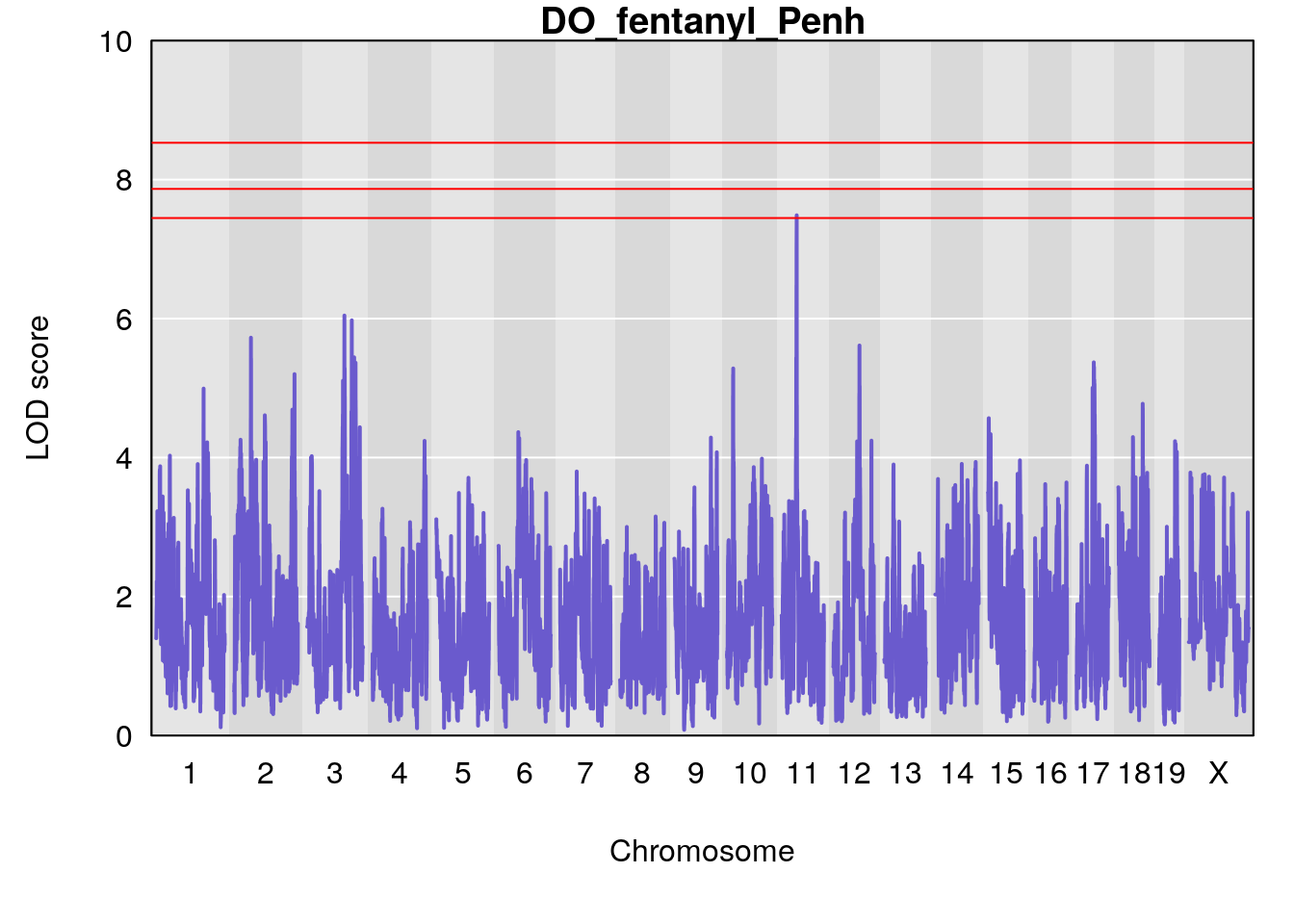
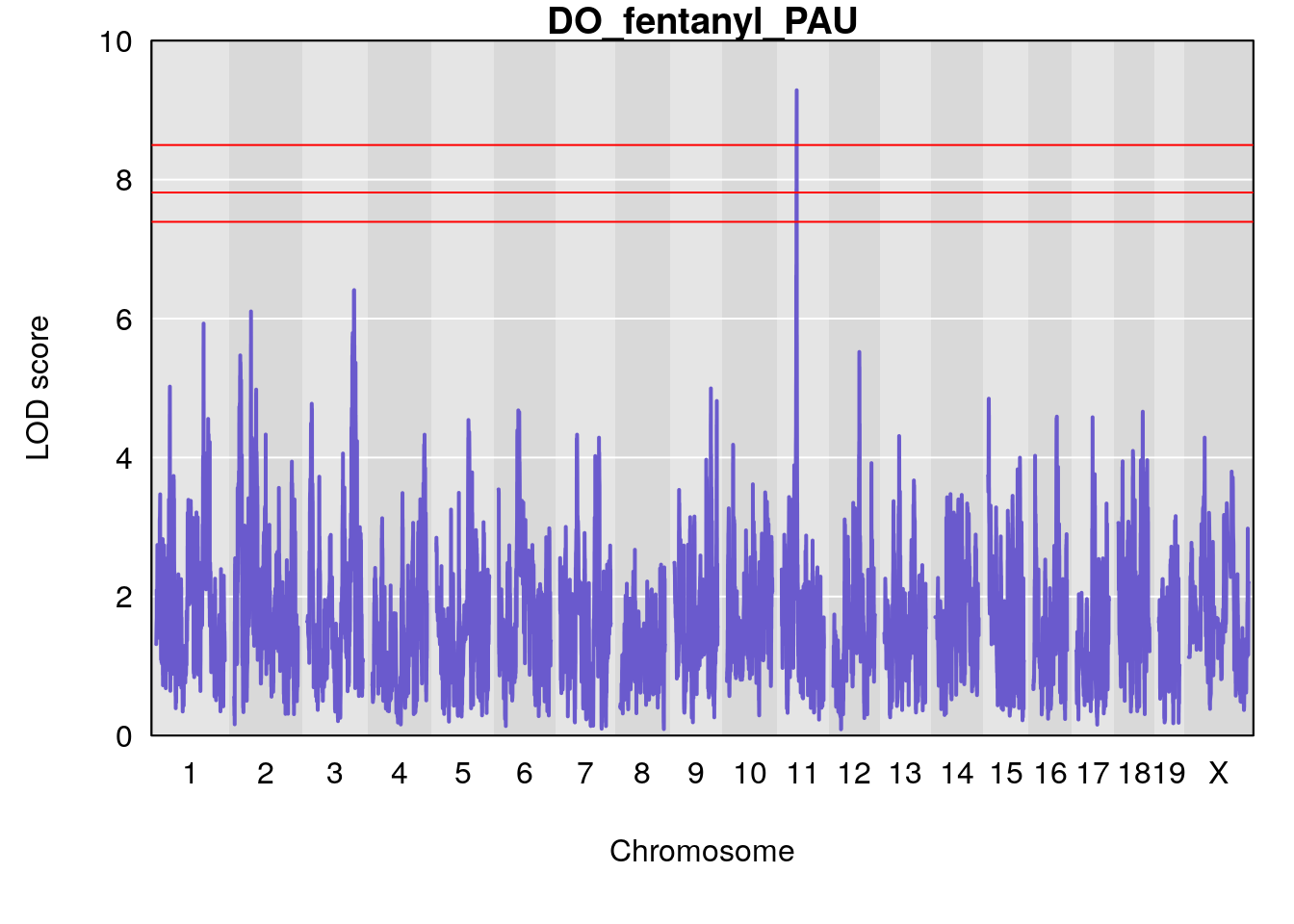
for(i in names(qtl.morphine.out)){
par(mar=c(5.1, 4.1, 1.1, 1.1))
ymx <- maxlod(qtl.morphine.out[[i]]) # overall maximum LOD score
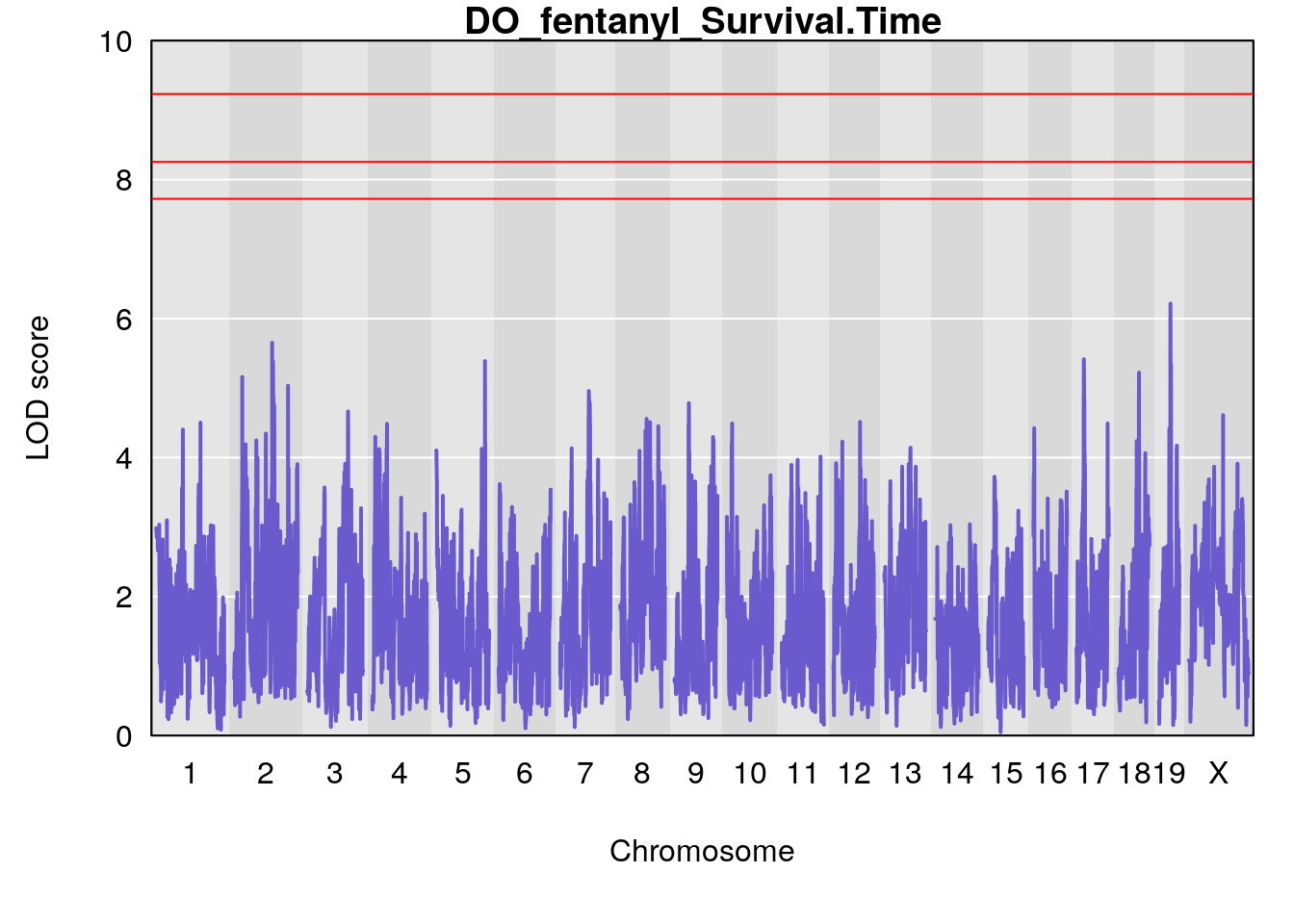
plot(qtl.morphine.out[[i]], map=gm$pmap, lodcolumn=1, col="slateblue", ylim=c(0, 10))
abline(h=summary(qtl.morphine.operm[[i]], alpha=c(0.10, 0.05, 0.01))[[1]], col="red")
abline(h=summary(qtl.morphine.operm[[i]], alpha=c(0.10, 0.05, 0.01))[[2]], col="red")
abline(h=summary(qtl.morphine.operm[[i]], alpha=c(0.10, 0.05, 0.01))[[3]], col="red")
title(main = paste0("DO_fentanyl_",i))
}


#save genome-wide plot
for(i in names(qtl.morphine.out)){
png(file = paste0("output/Fentanyl/DO_fentanyl_", i, ".png"), width = 16, height =8, res=300, units = "in")
par(mar=c(5.1, 4.1, 1.1, 1.1))
ymx <- maxlod(qtl.morphine.out[[i]]) # overall maximum LOD score
plot(qtl.morphine.out[[i]], map=gm$pmap, lodcolumn=1, col="slateblue", ylim=c(0, 10))
abline(h=summary(qtl.morphine.operm[[i]], alpha=c(0.10, 0.05, 0.01))[[1]], col="red")
abline(h=summary(qtl.morphine.operm[[i]], alpha=c(0.10, 0.05, 0.01))[[2]], col="red")
abline(h=summary(qtl.morphine.operm[[i]], alpha=c(0.10, 0.05, 0.01))[[3]], col="red")
title(main = paste0("DO_fentanyl_",i))
dev.off()
}
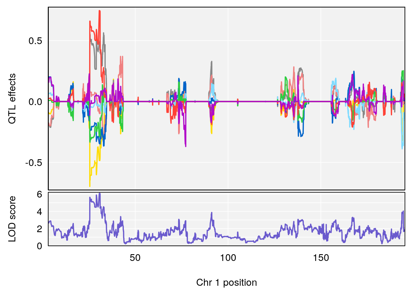
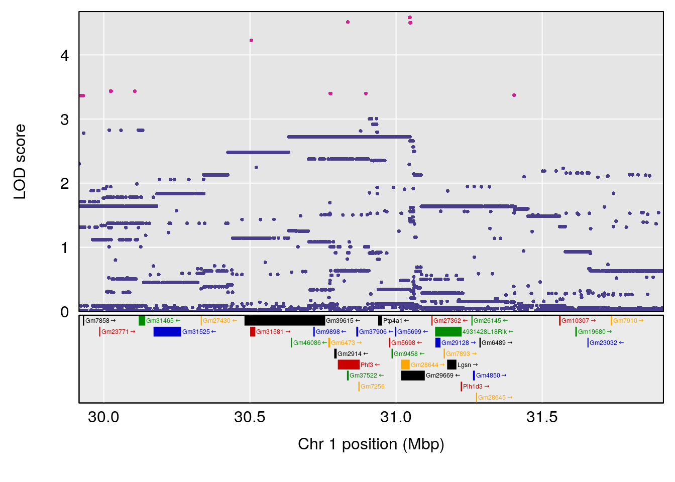
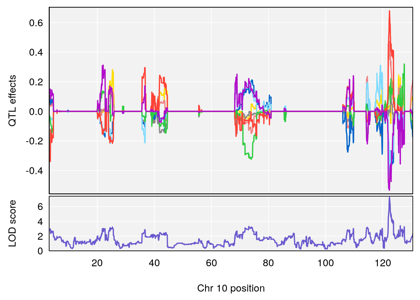
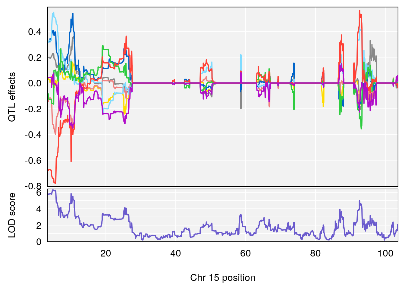
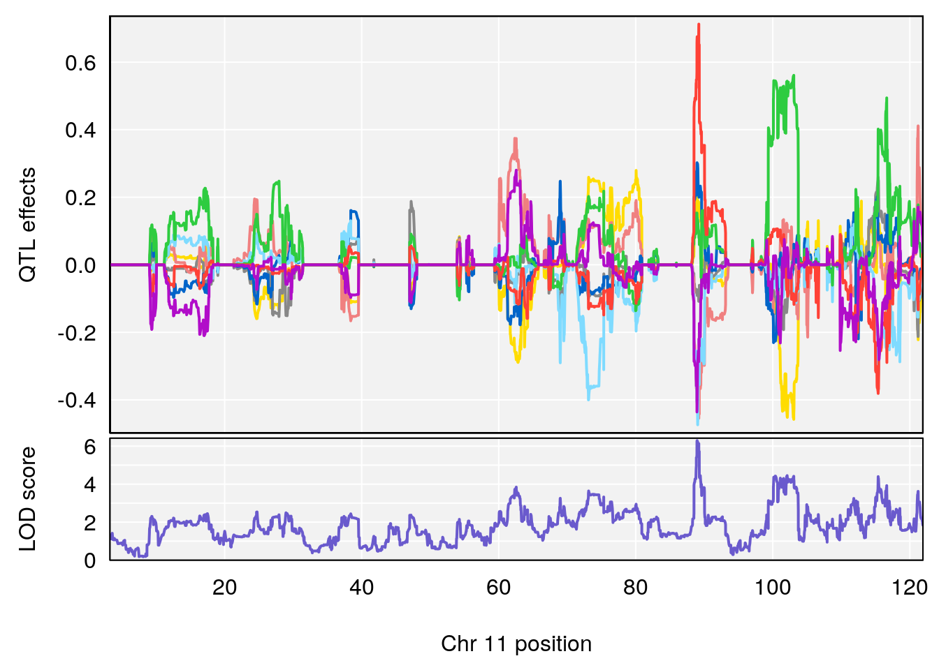
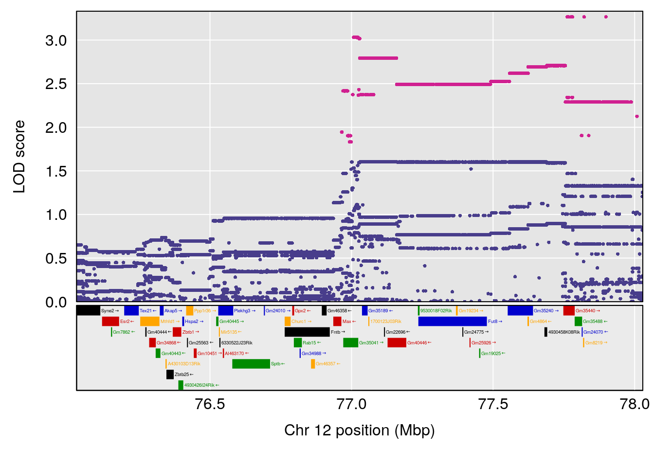
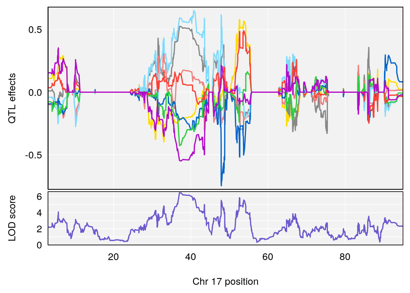
#peaks coeff plot
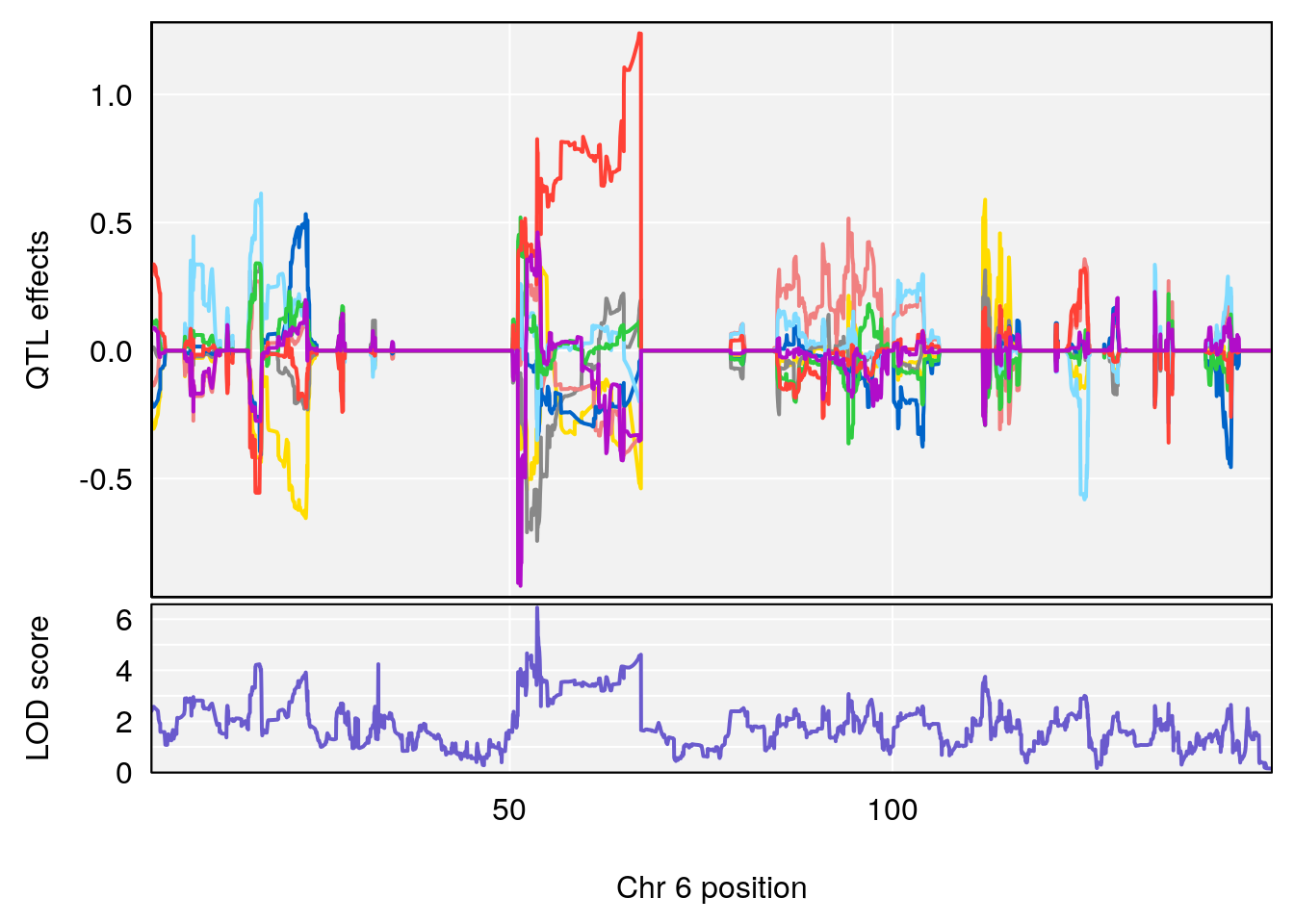
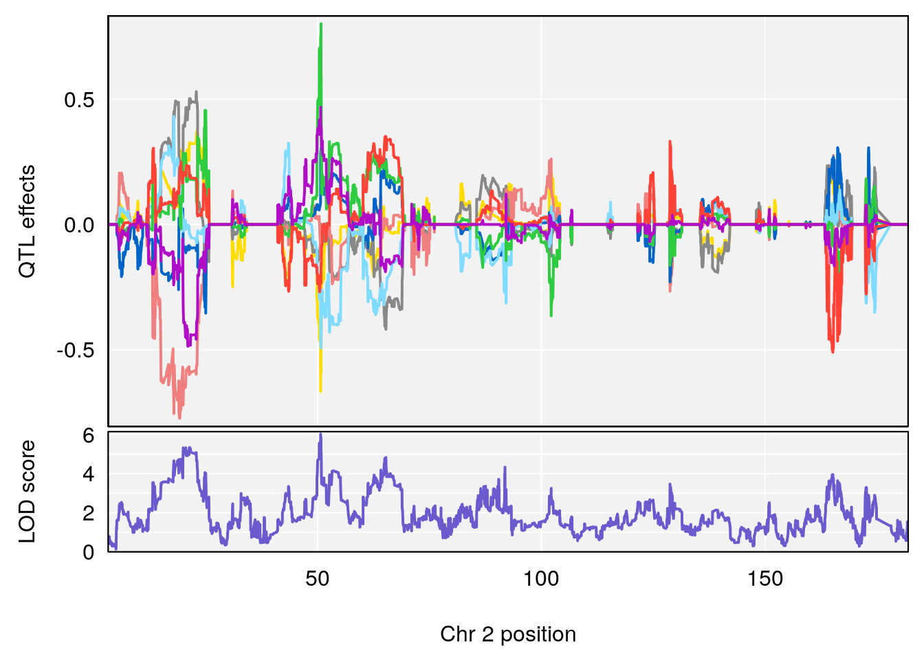
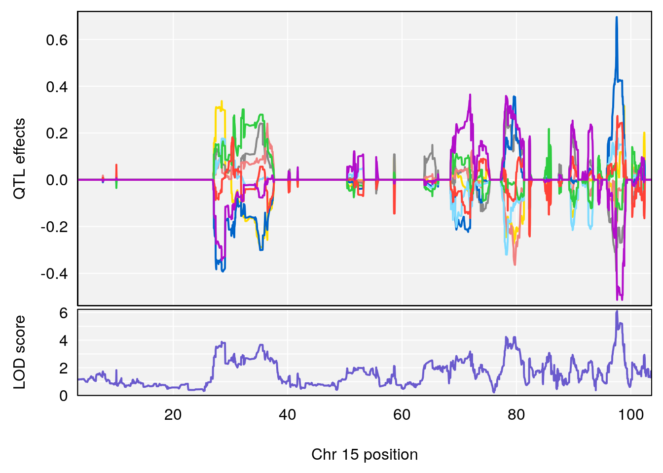
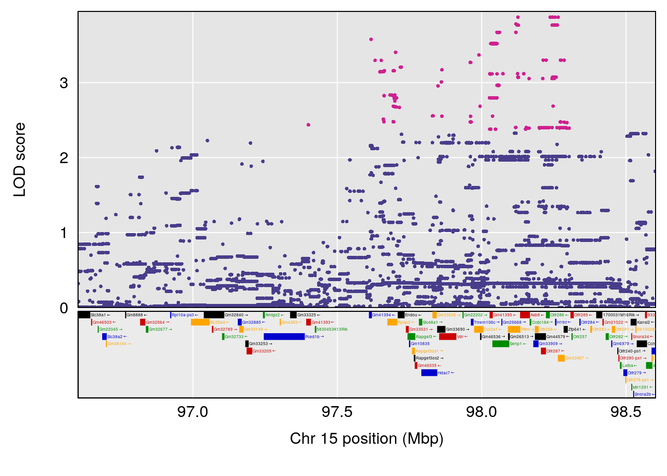
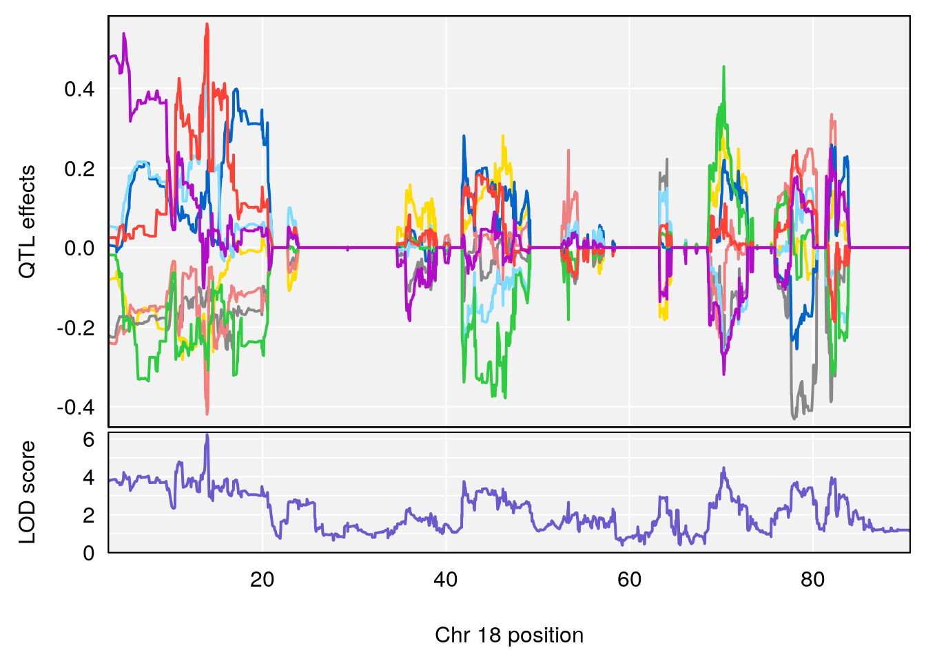
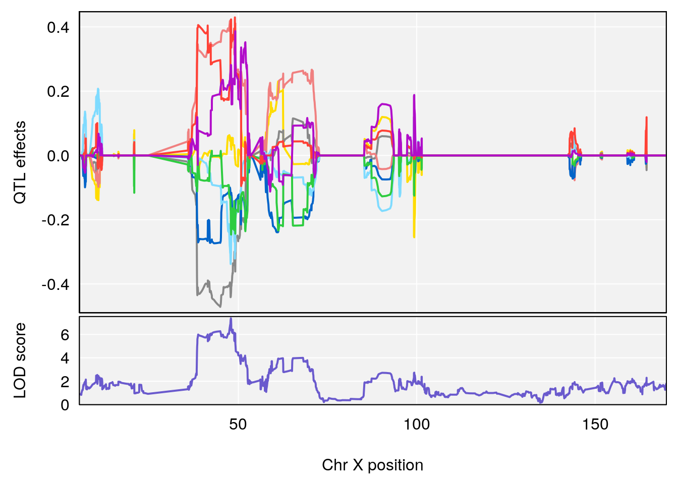
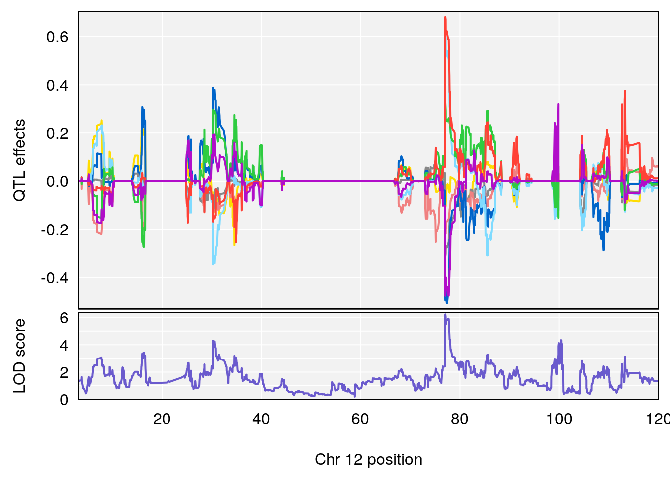
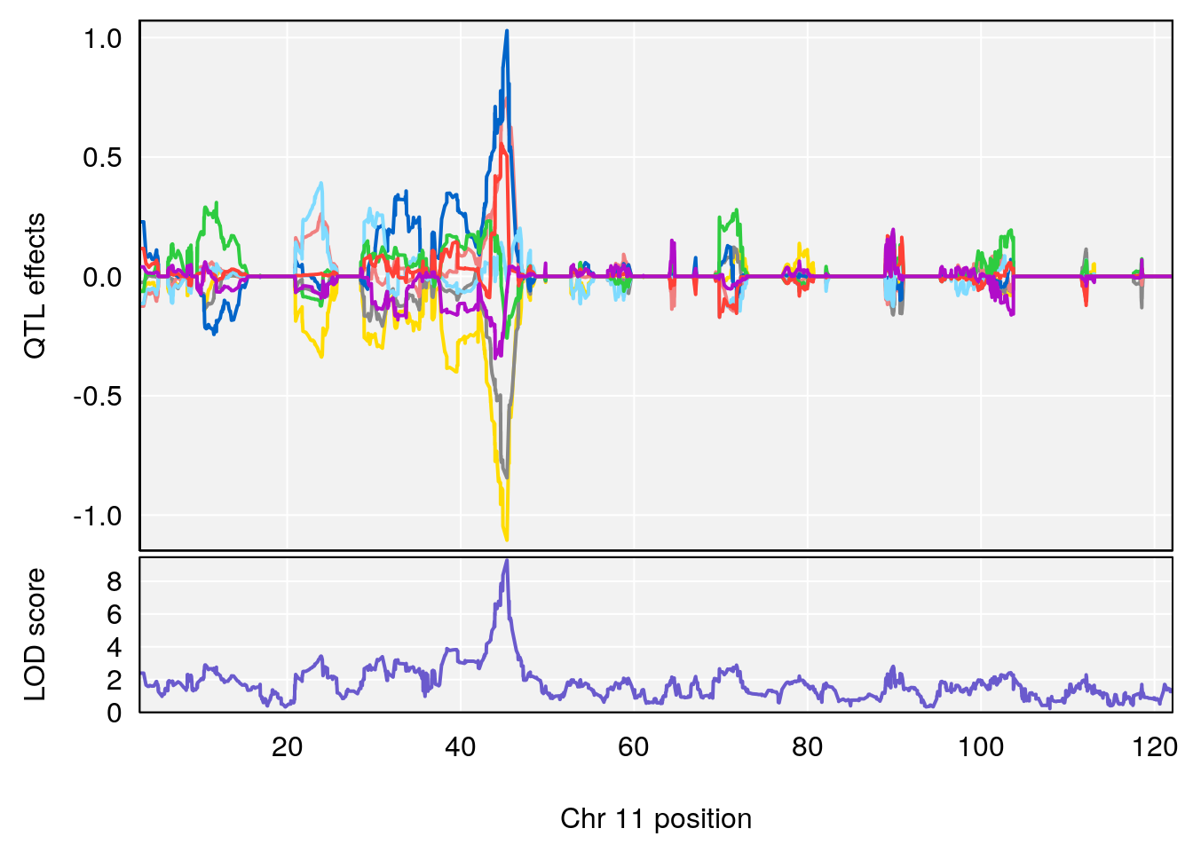
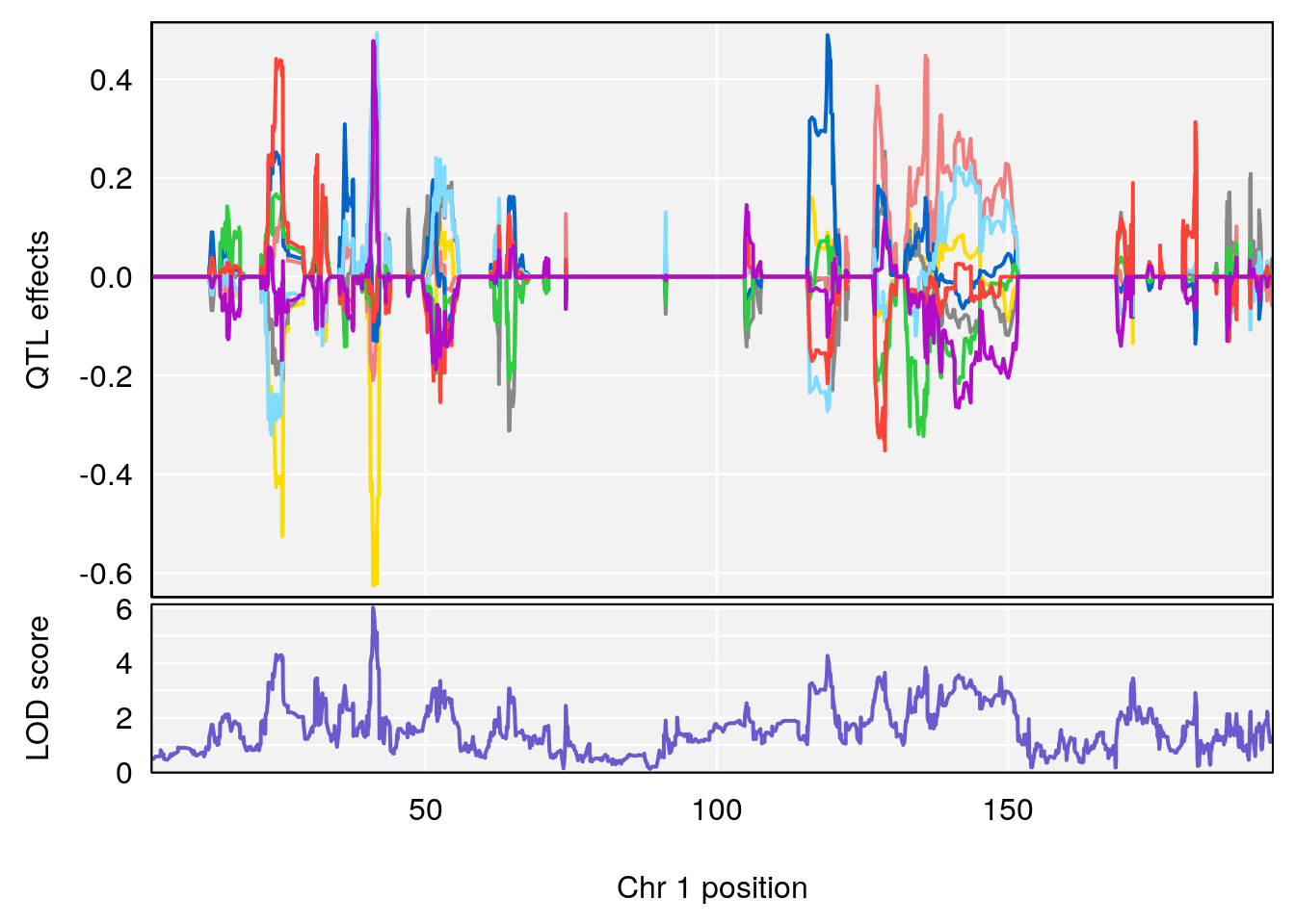
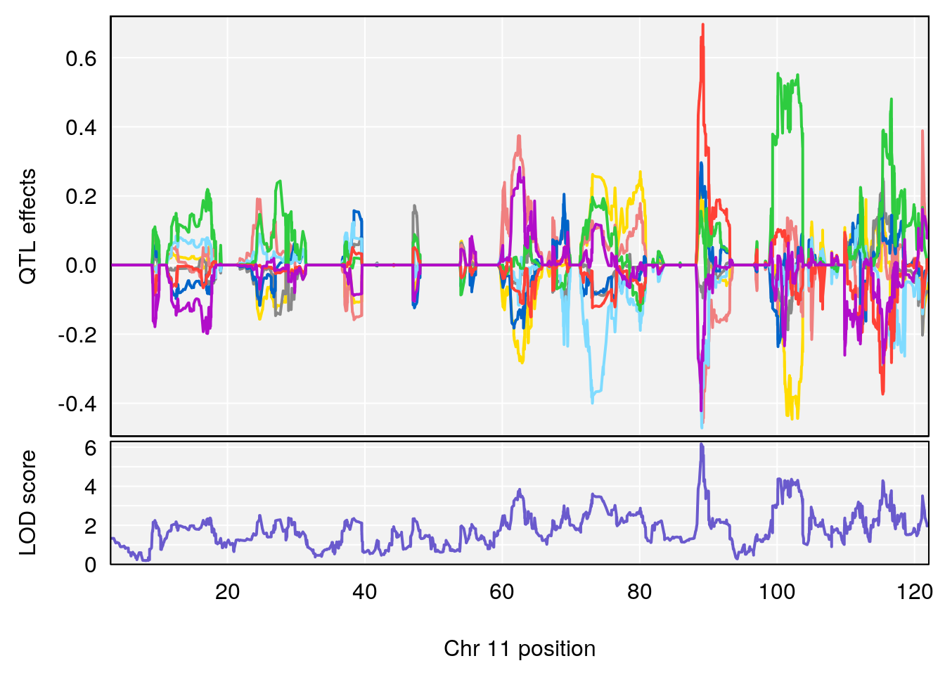
for(i in names(qtl.morphine.out)){
print(i)
peaks <- find_peaks(qtl.morphine.out[[i]], map=gm$pmap, threshold=6, drop=1.5)
print(peaks)
if(dim(peaks)[1] != 0){
for(p in 1:dim(peaks)[1]) {
print(p)
chr <-peaks[p,3]
#coeff plot
par(mar=c(4.1, 4.1, 0.6, 0.6))
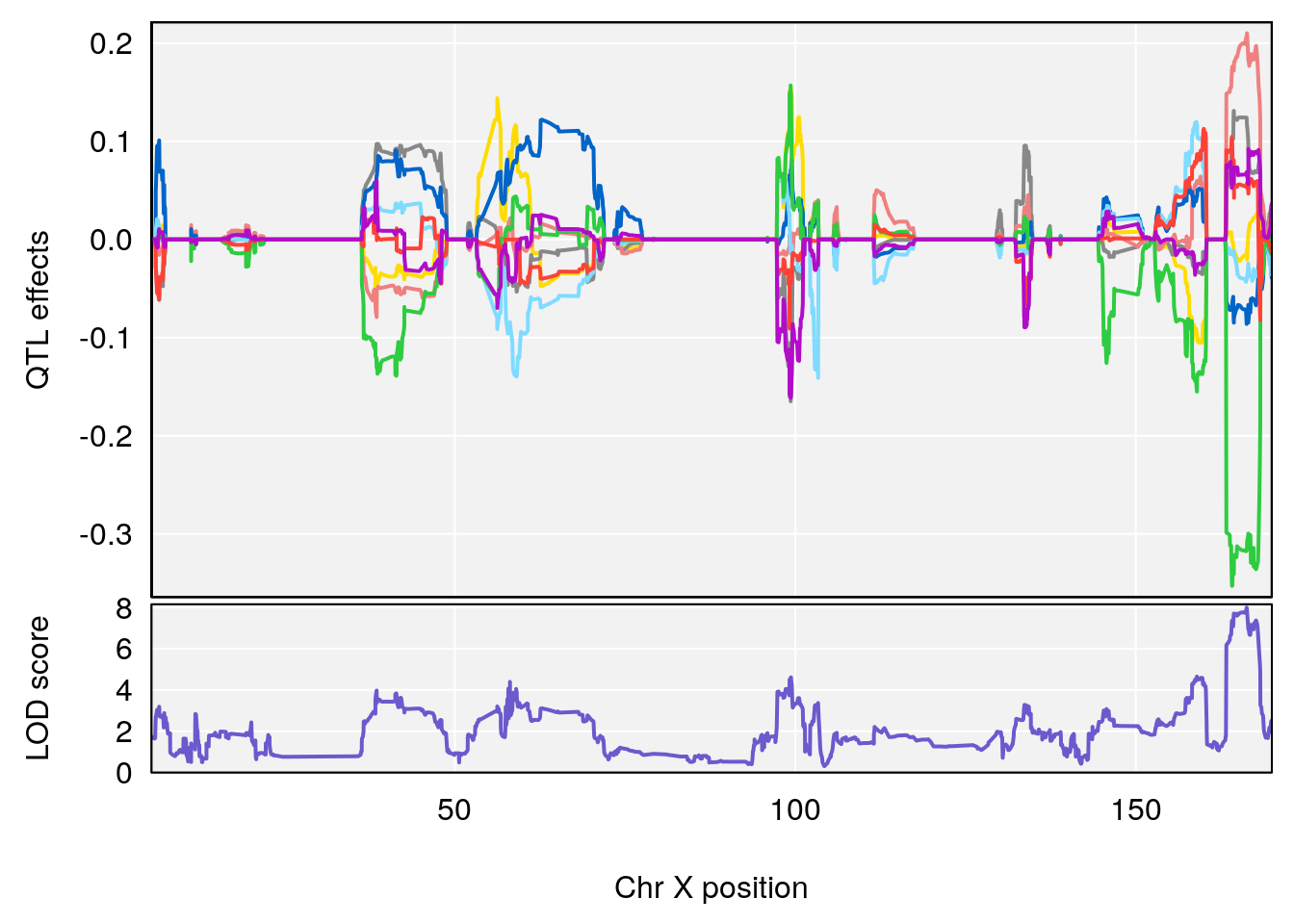
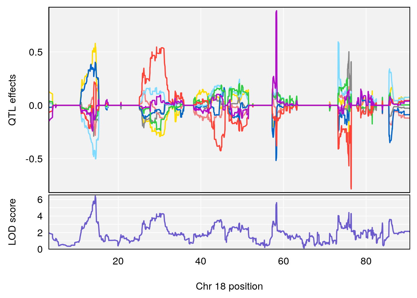
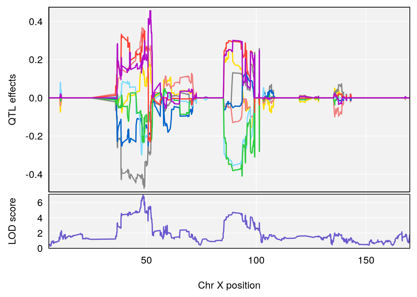
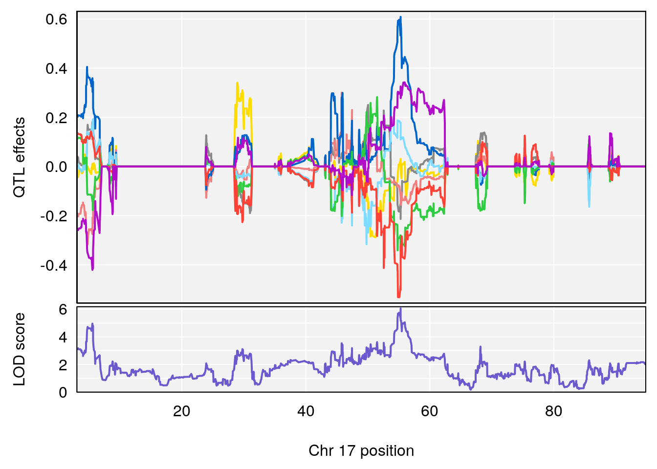
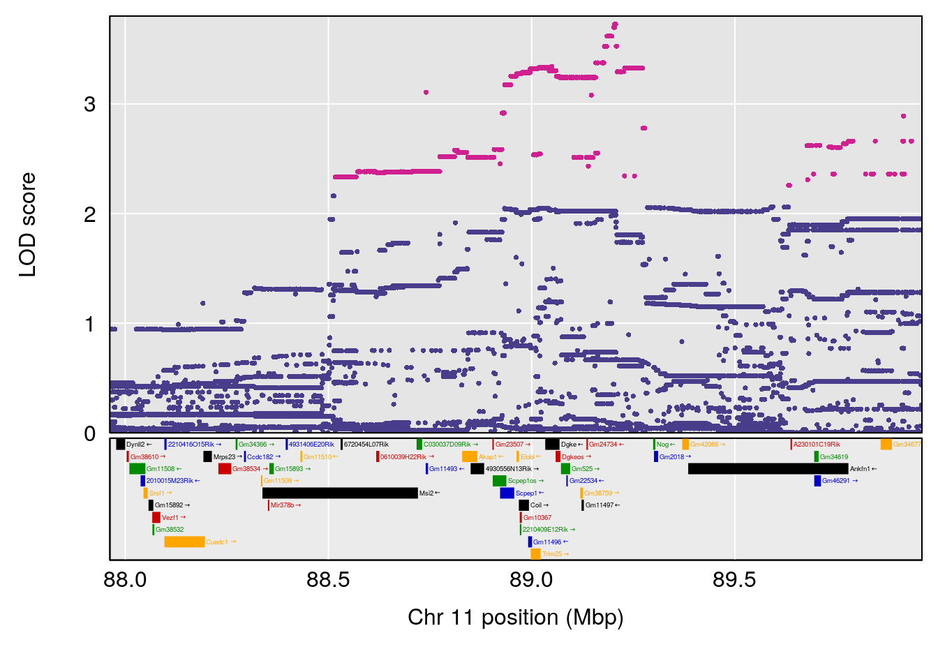
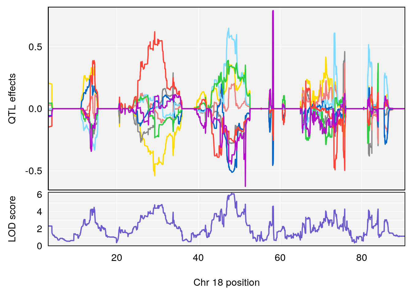
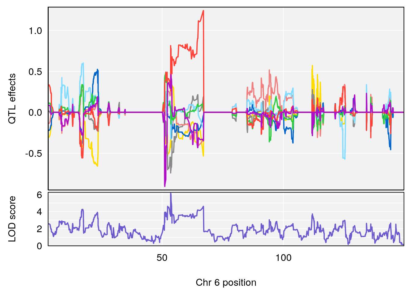
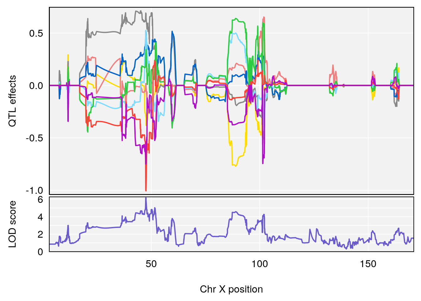
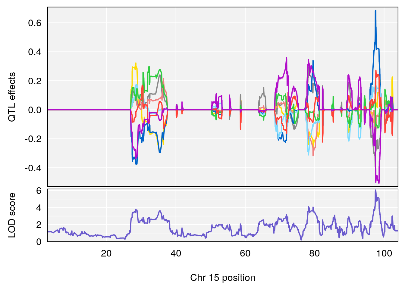
plot_coefCC(coef_c1[[i]][[p]], gm$pmap[chr], scan1_output=qtl.morphine.out[[i]], bgcolor="gray95", legend=NULL)
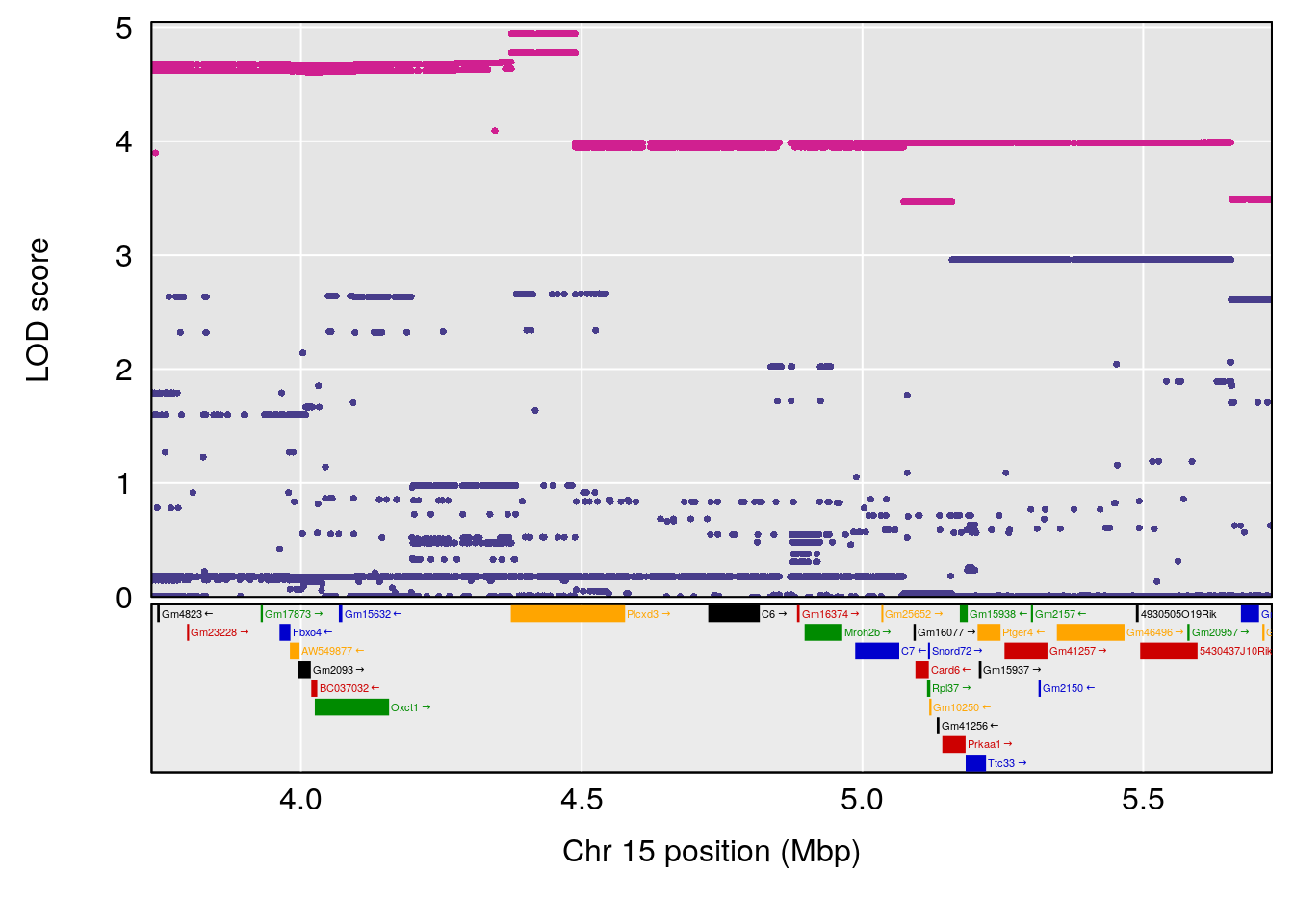
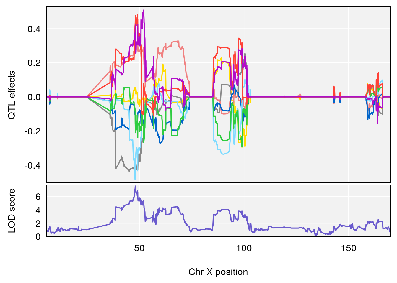
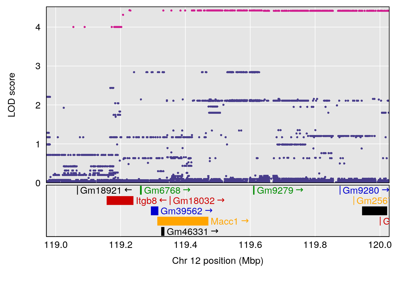
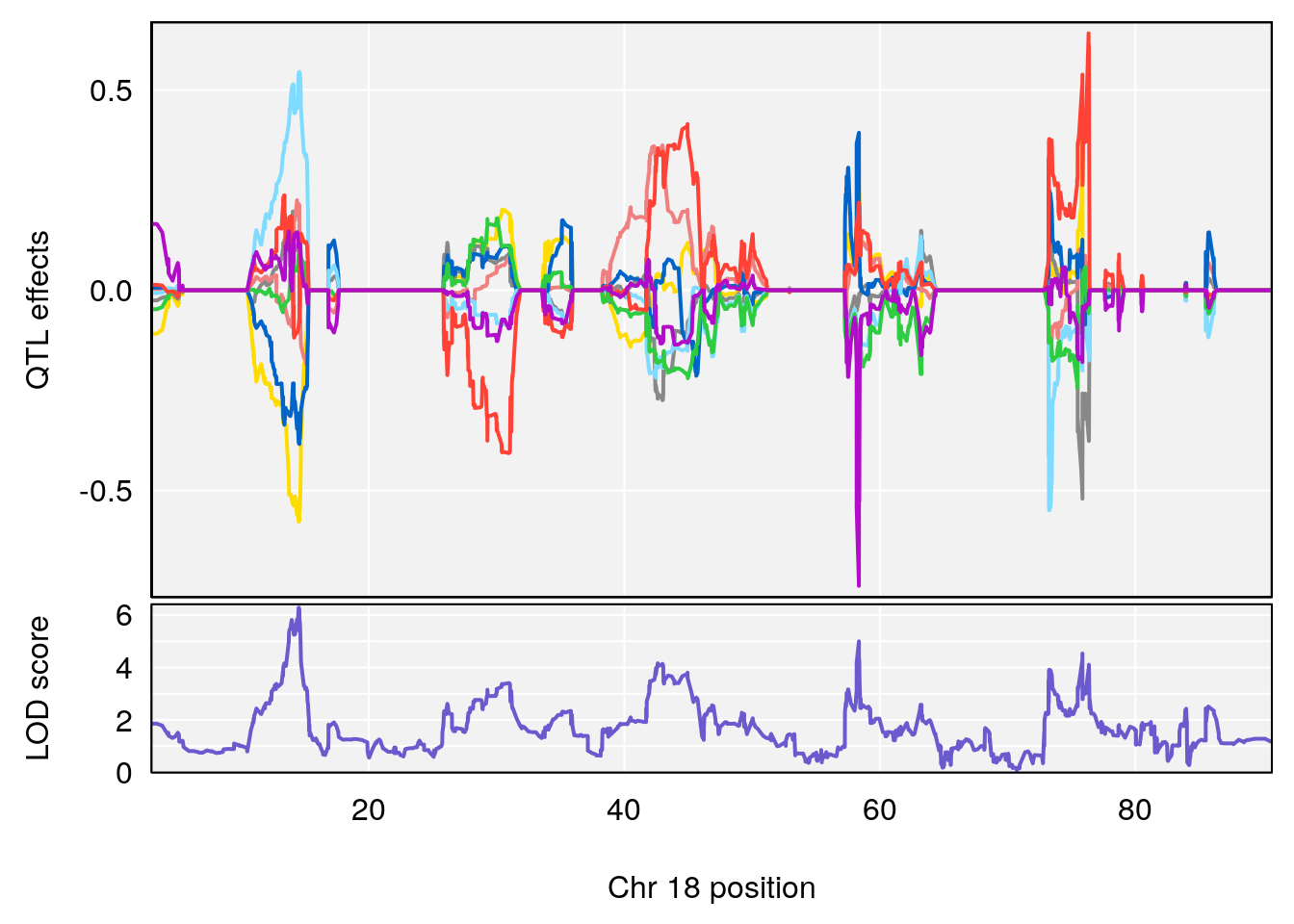
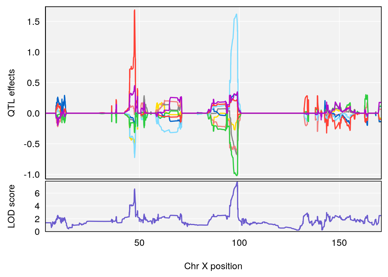
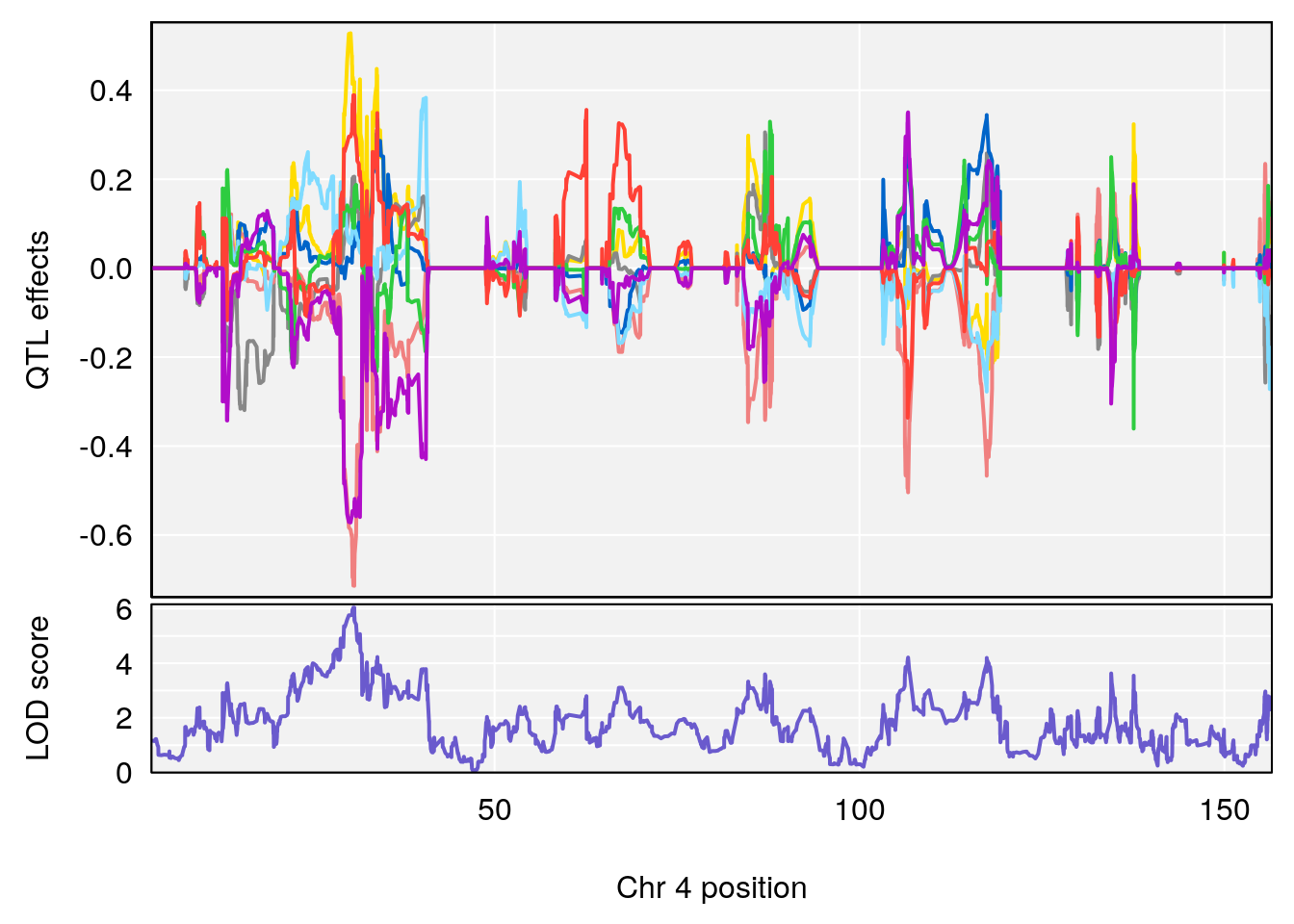
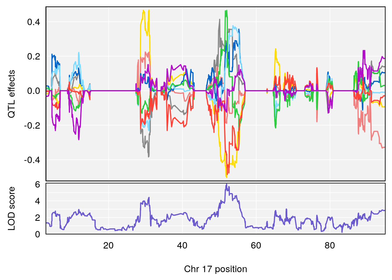
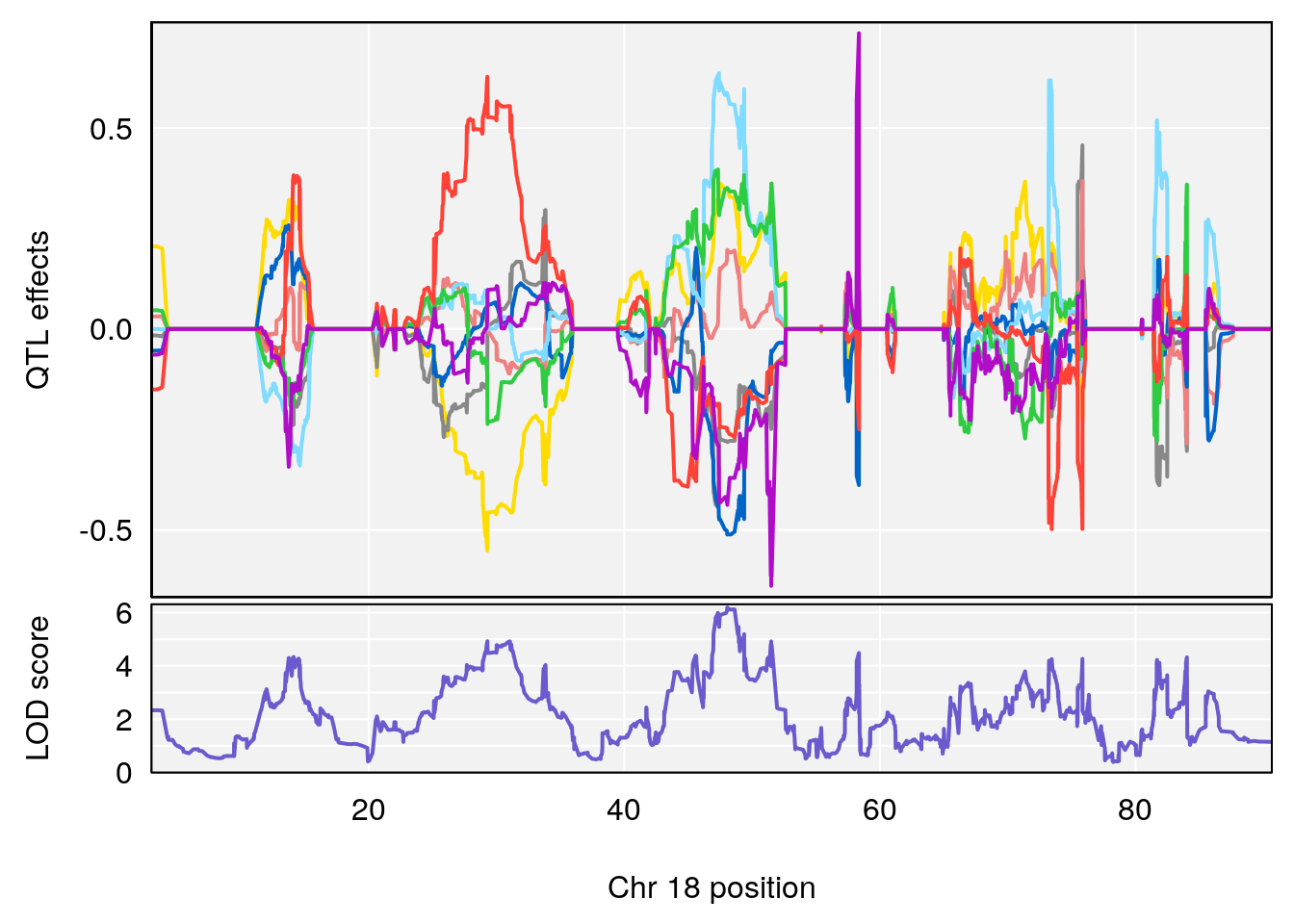
plot_coefCC(coef_c2[[i]][[p]], gm$pmap[chr], scan1_output=qtl.morphine.out[[i]], bgcolor="gray95", legend=NULL)
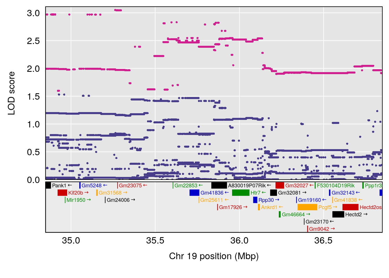
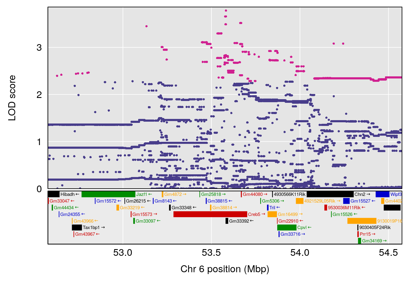
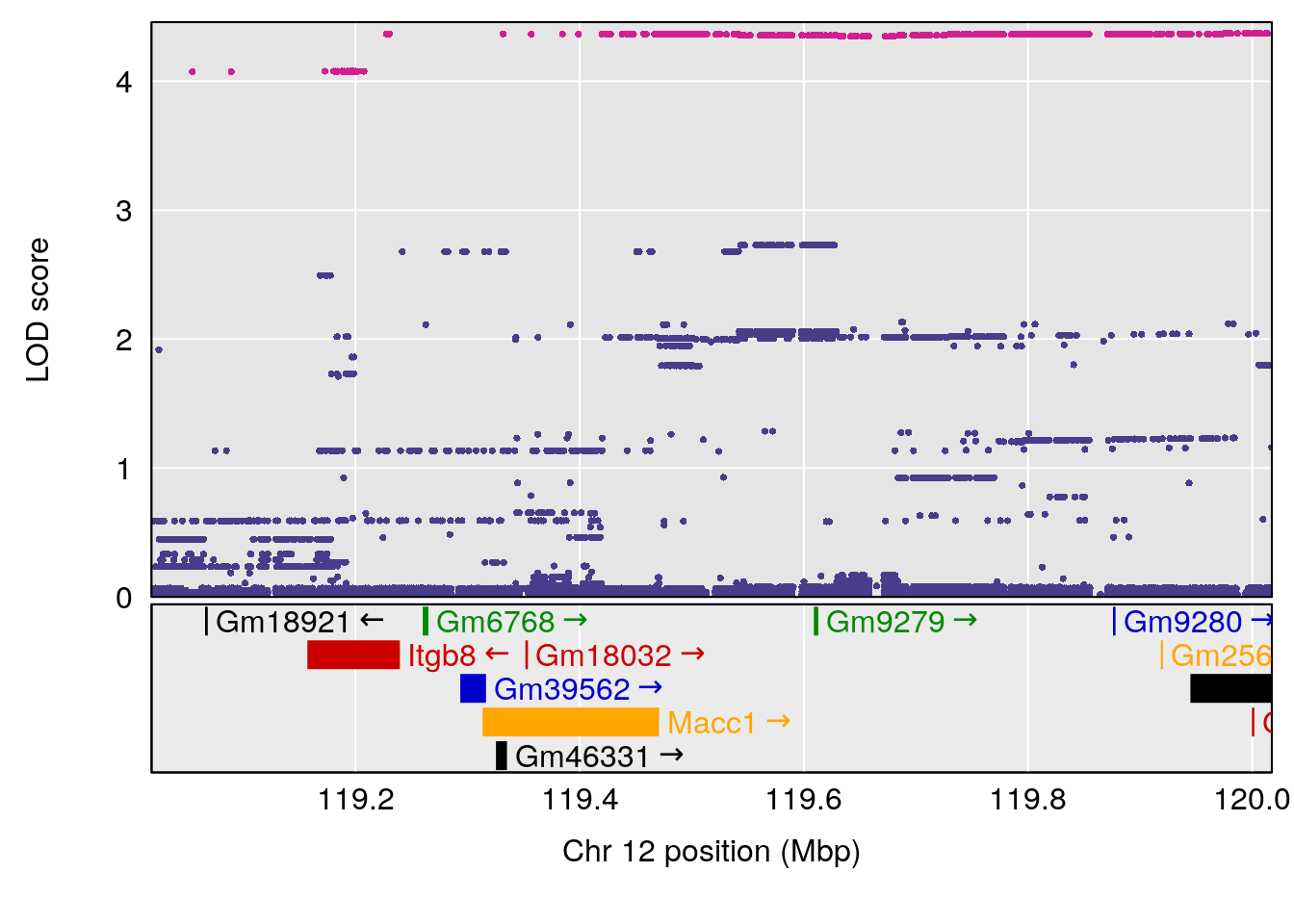
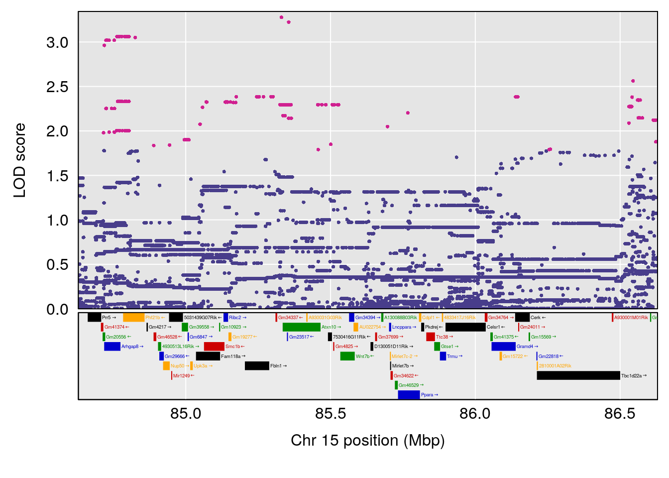
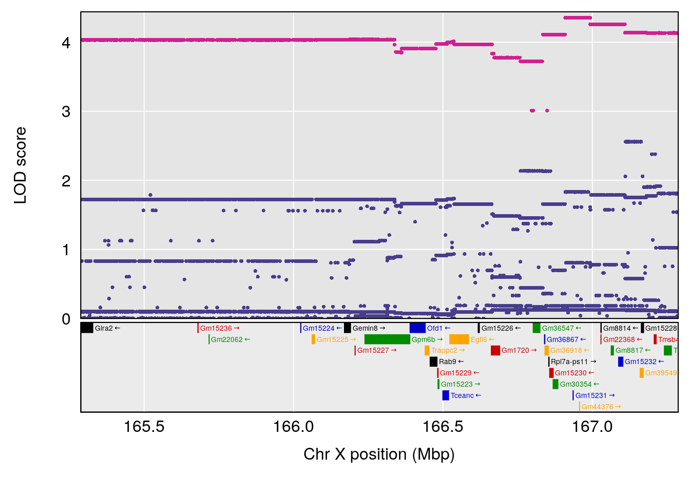
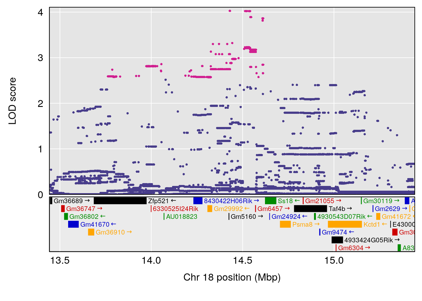
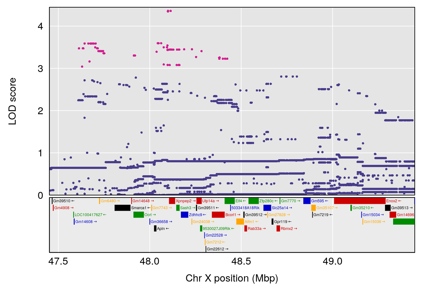
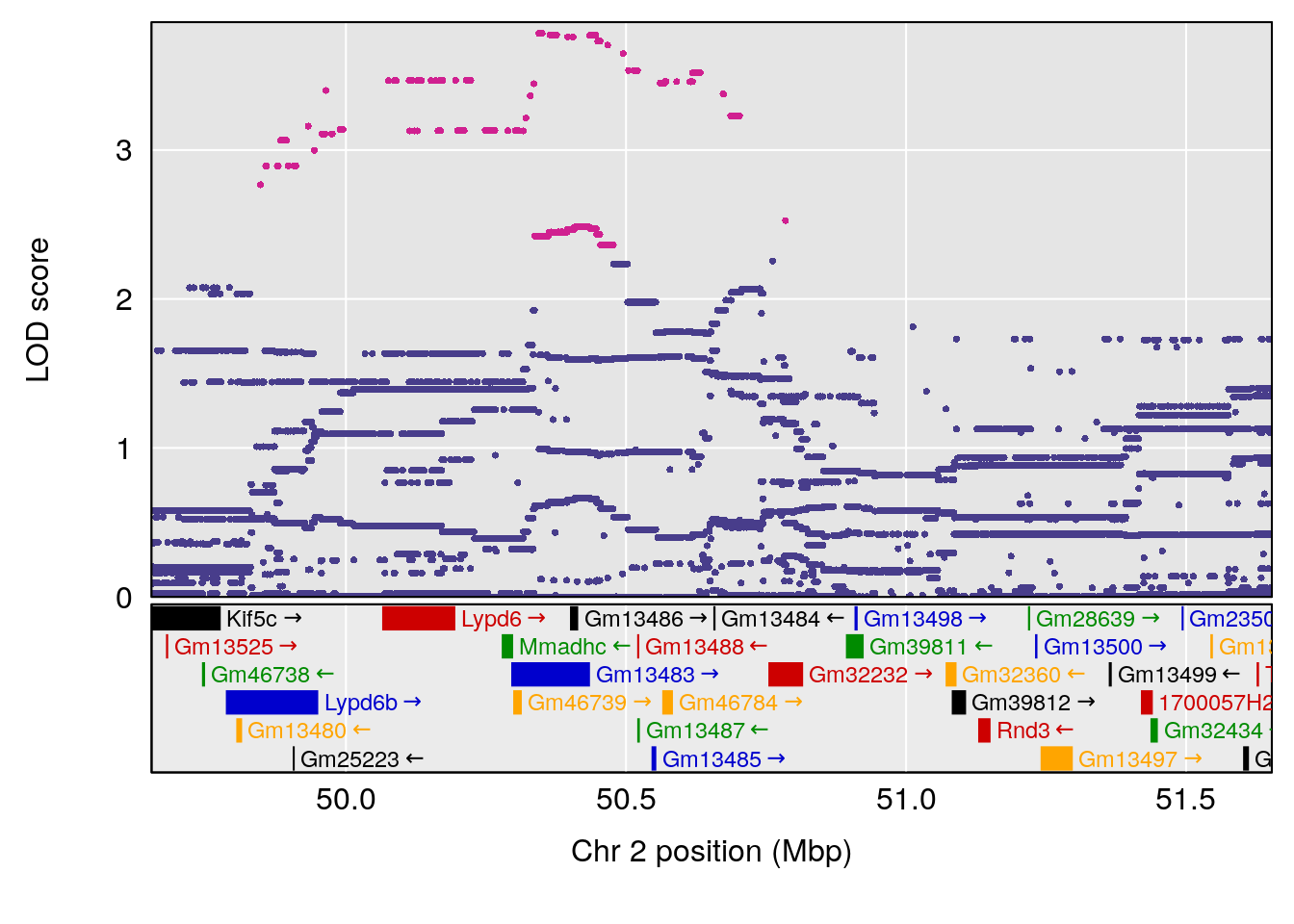
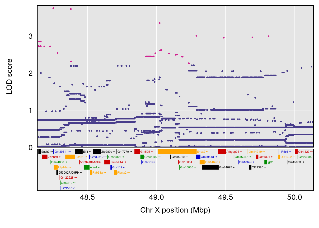
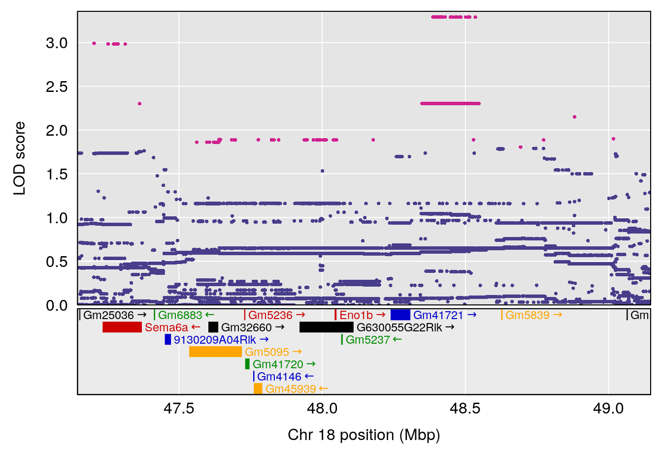
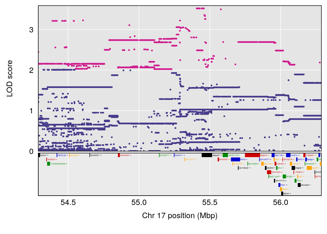
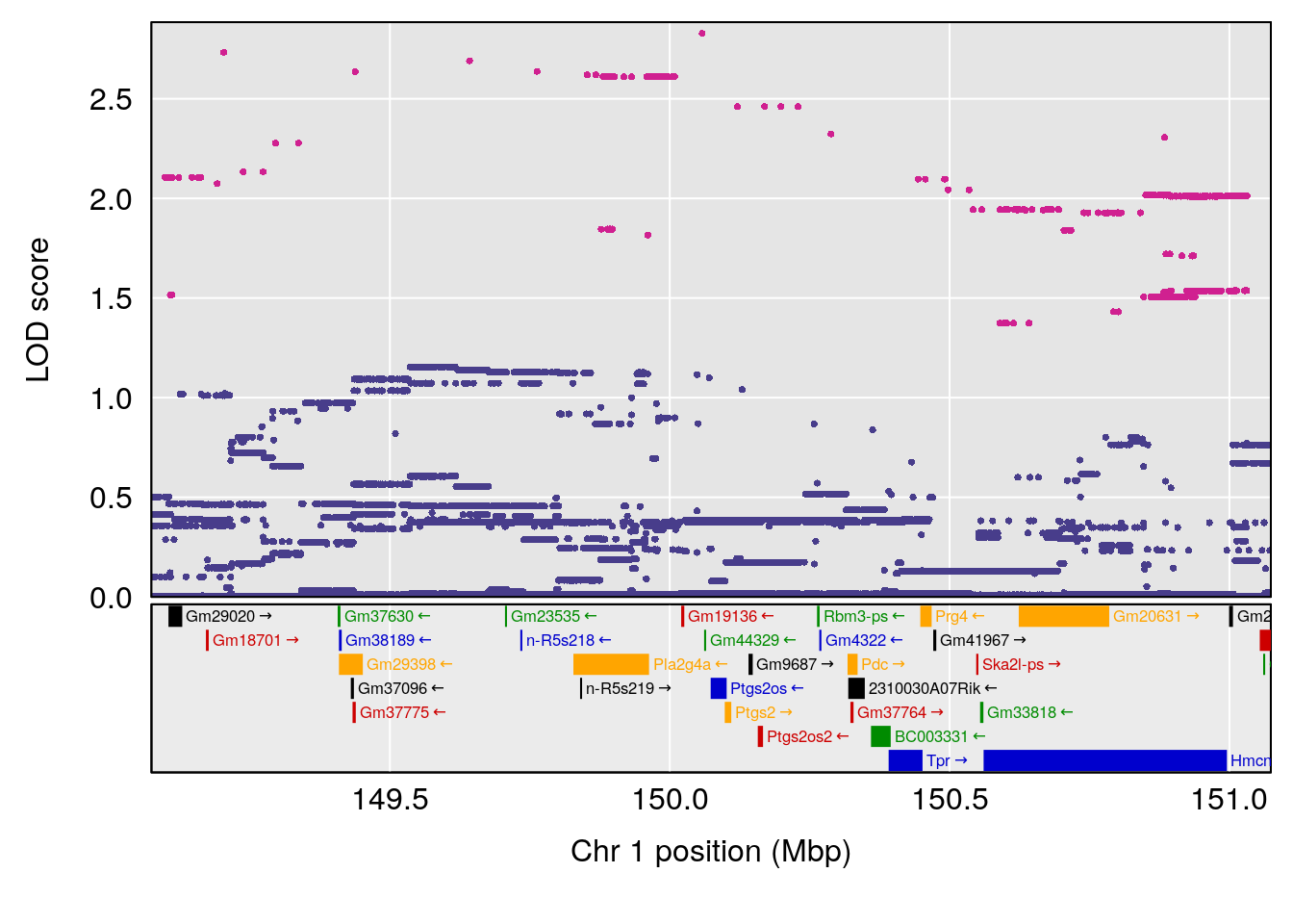
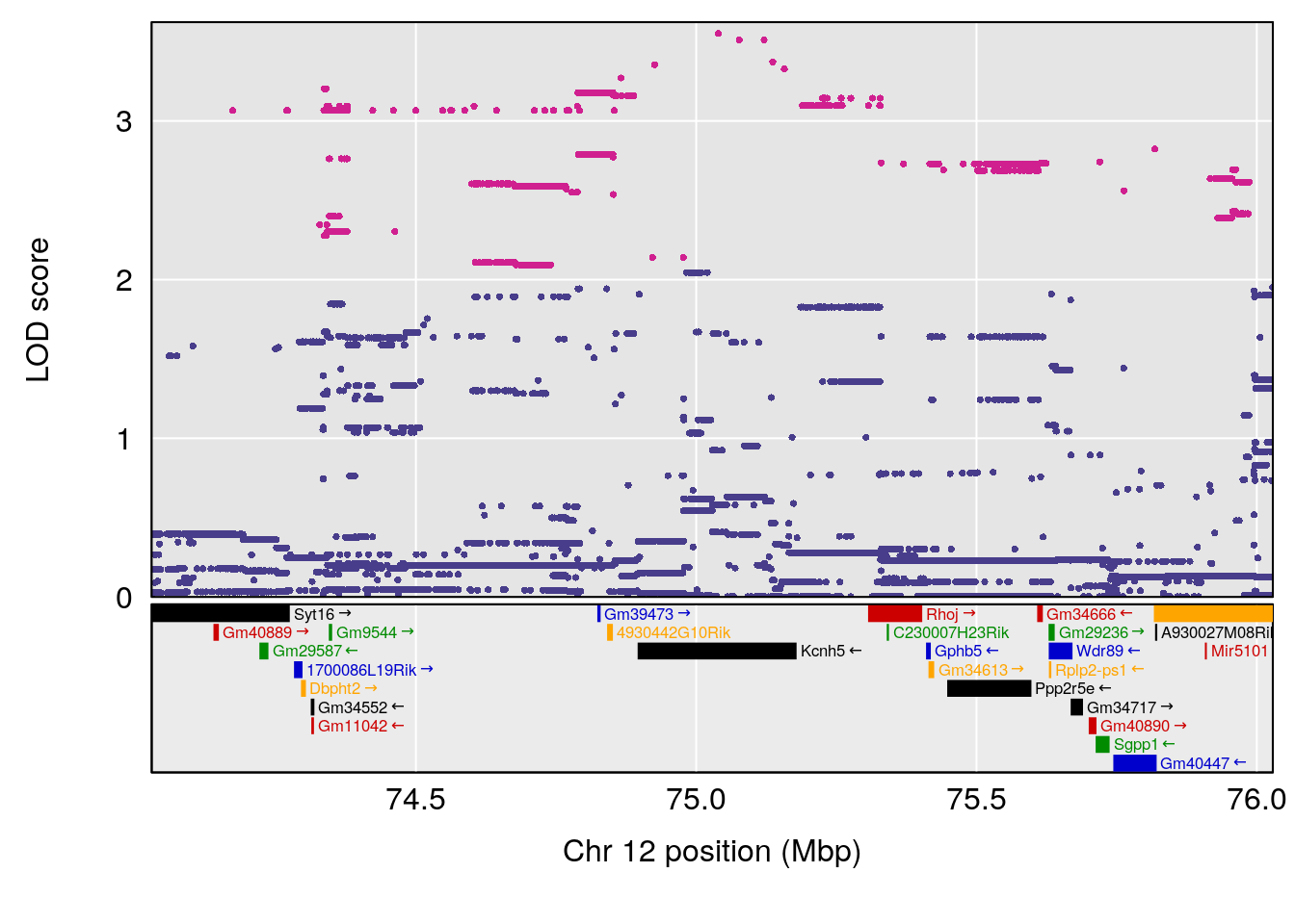
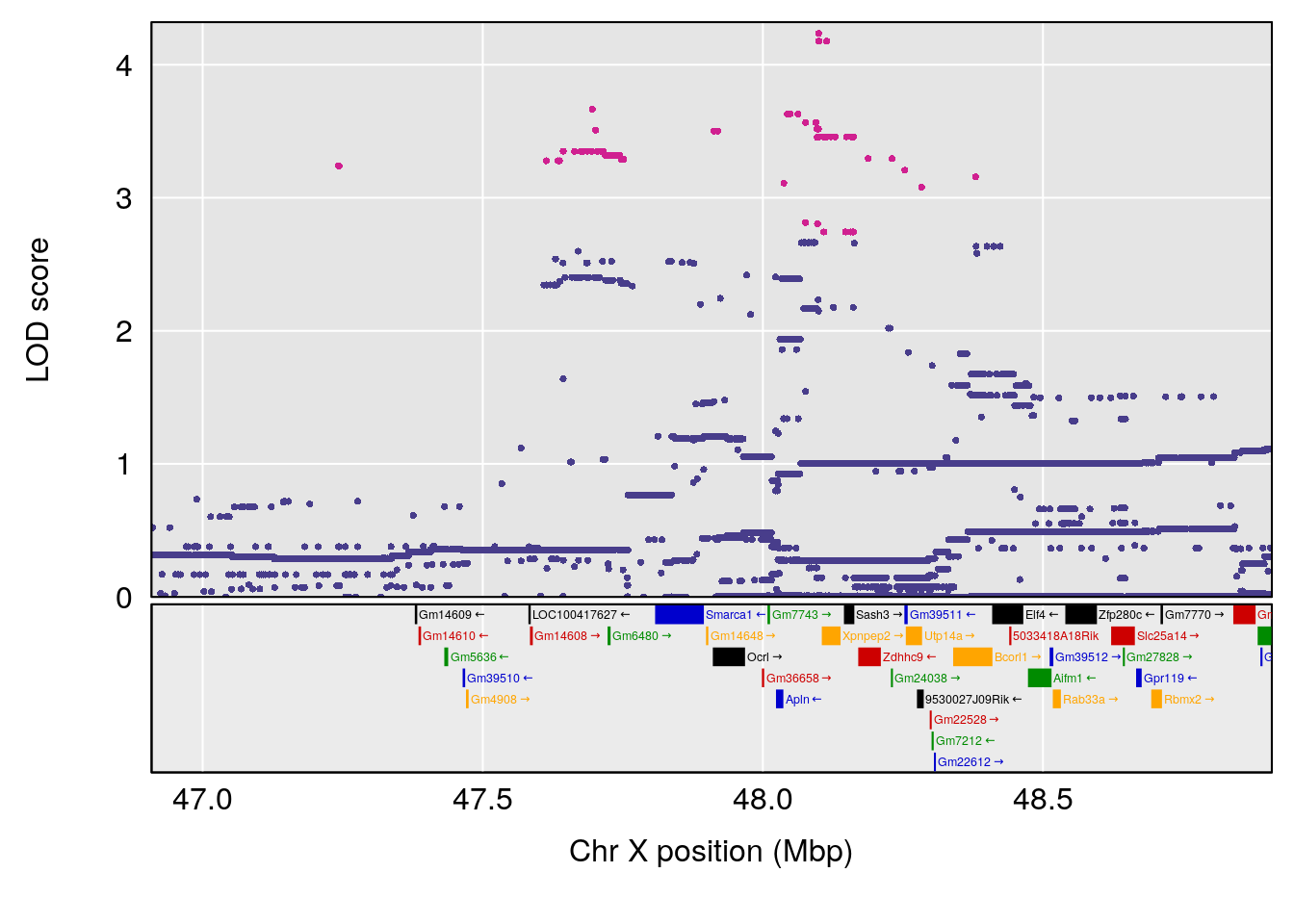
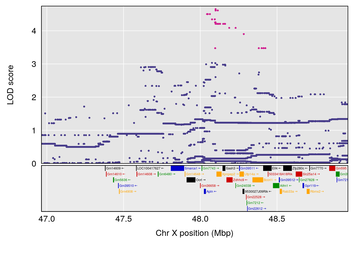
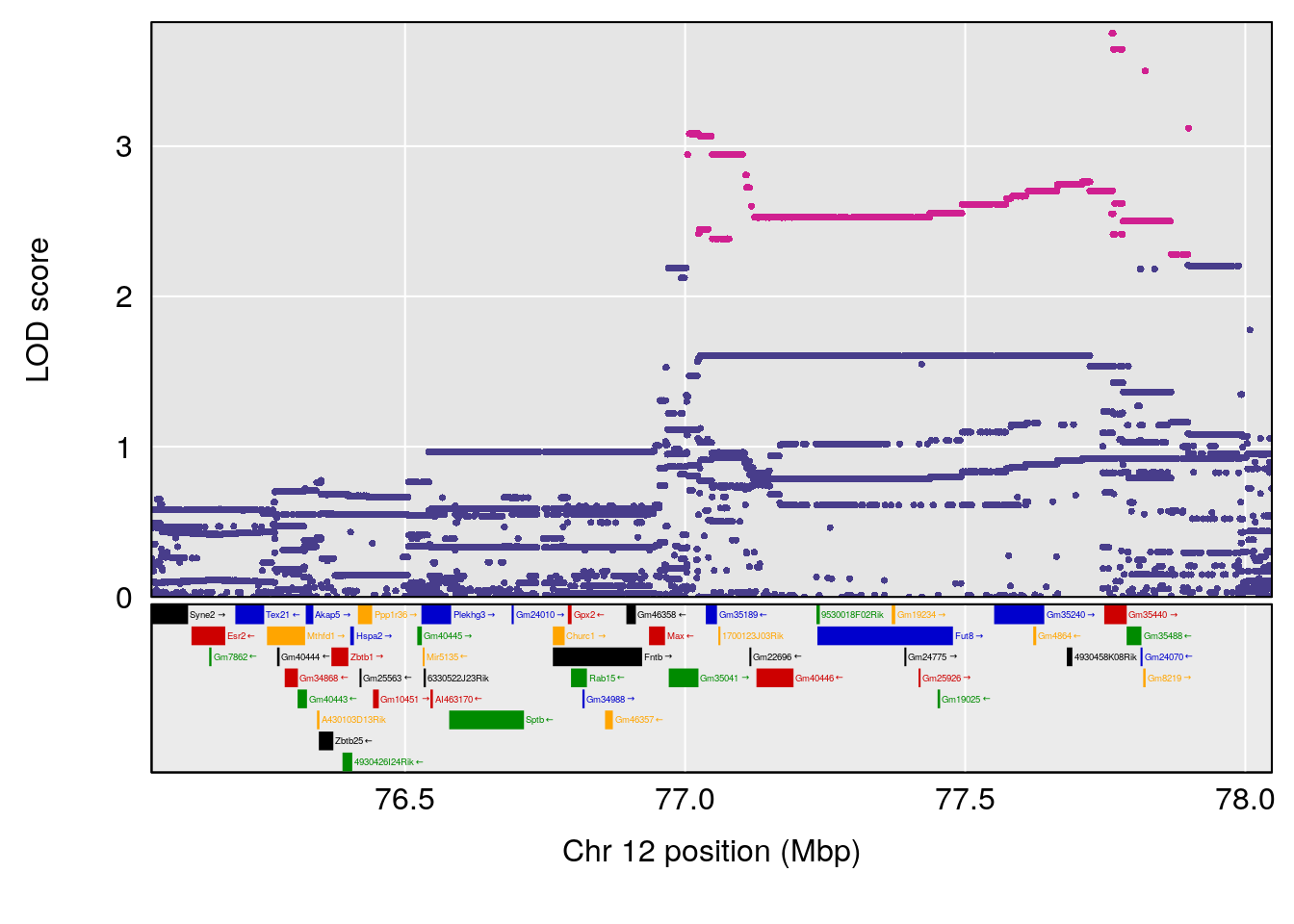
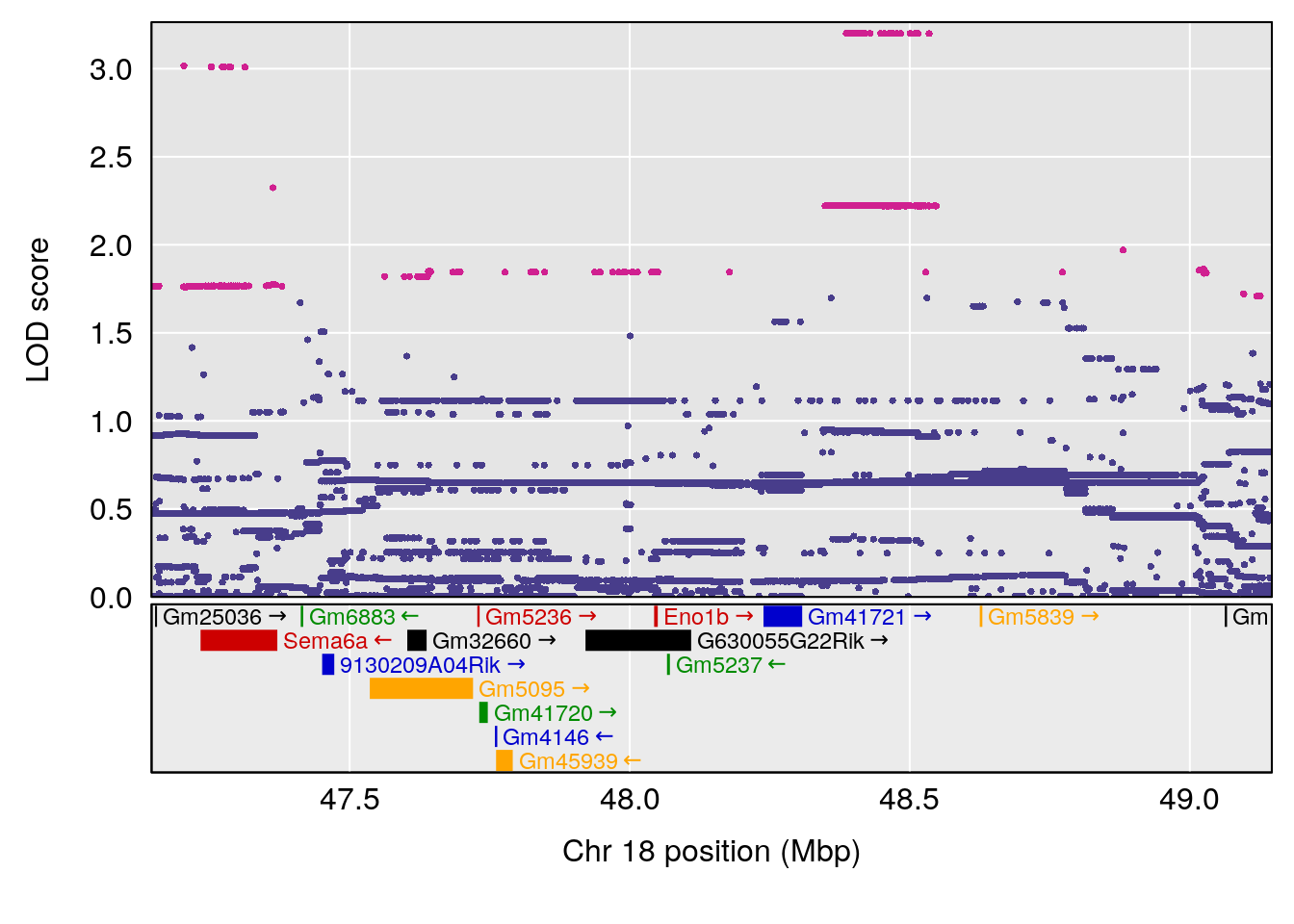
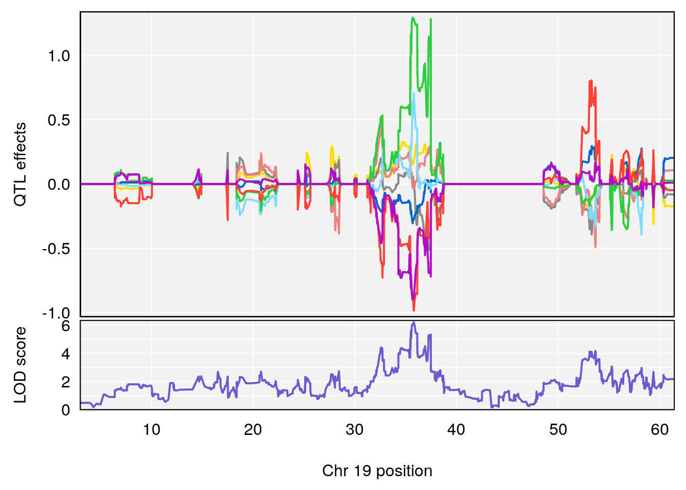
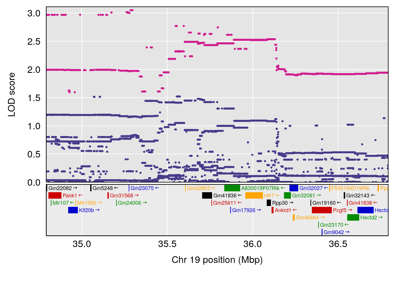
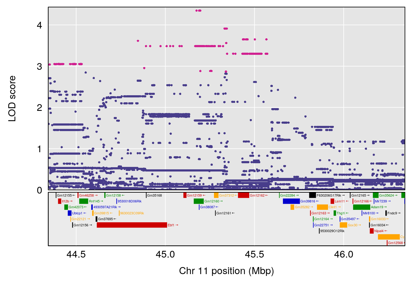
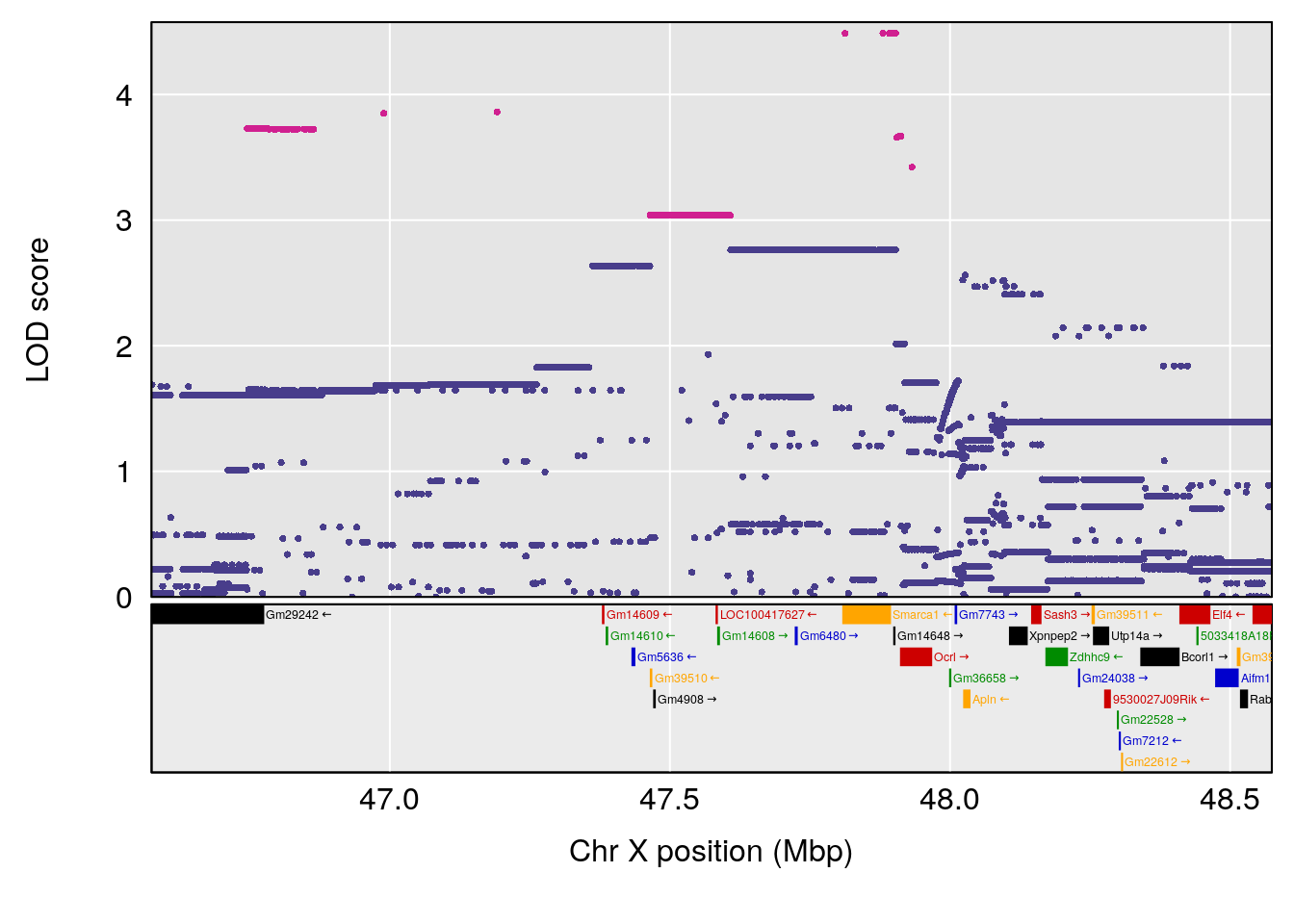
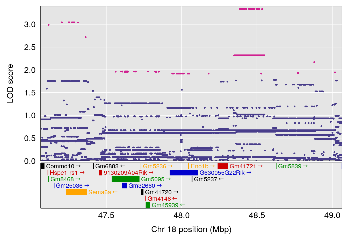
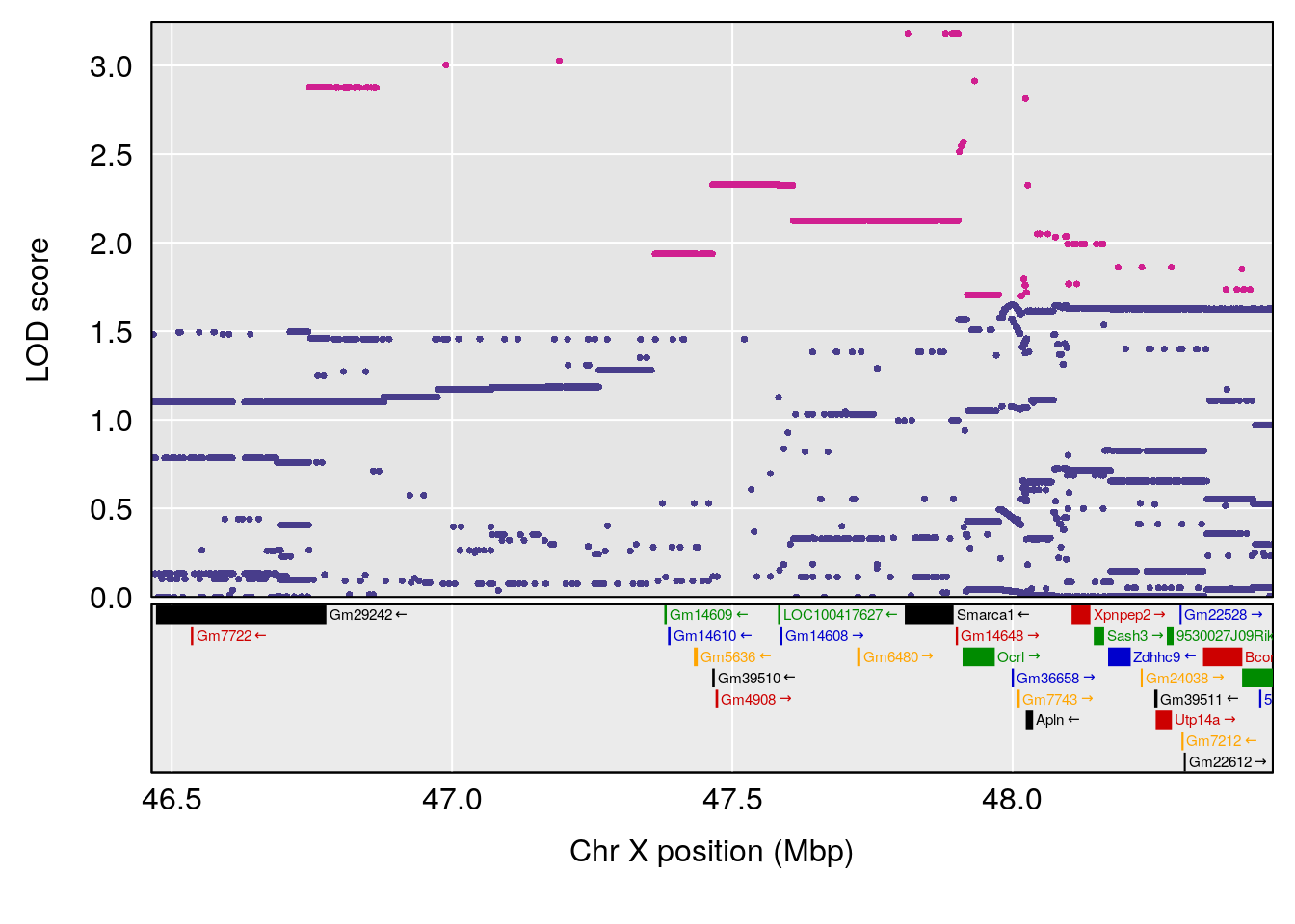
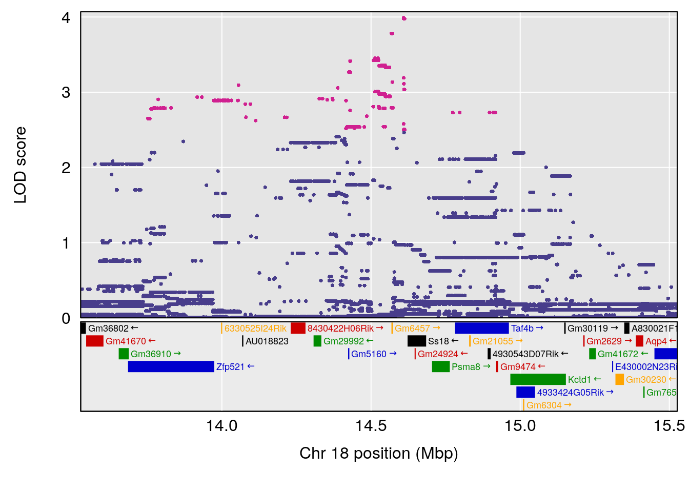
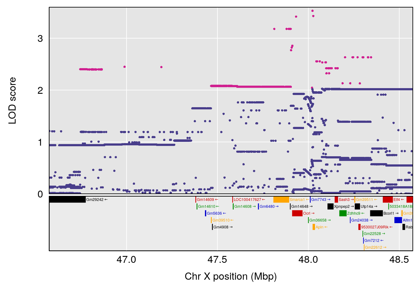
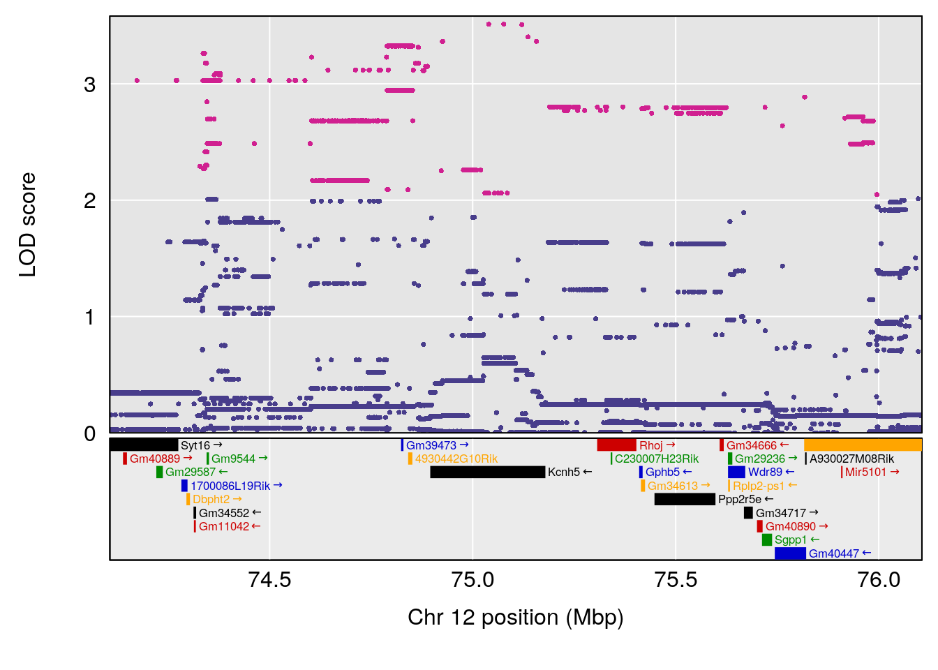
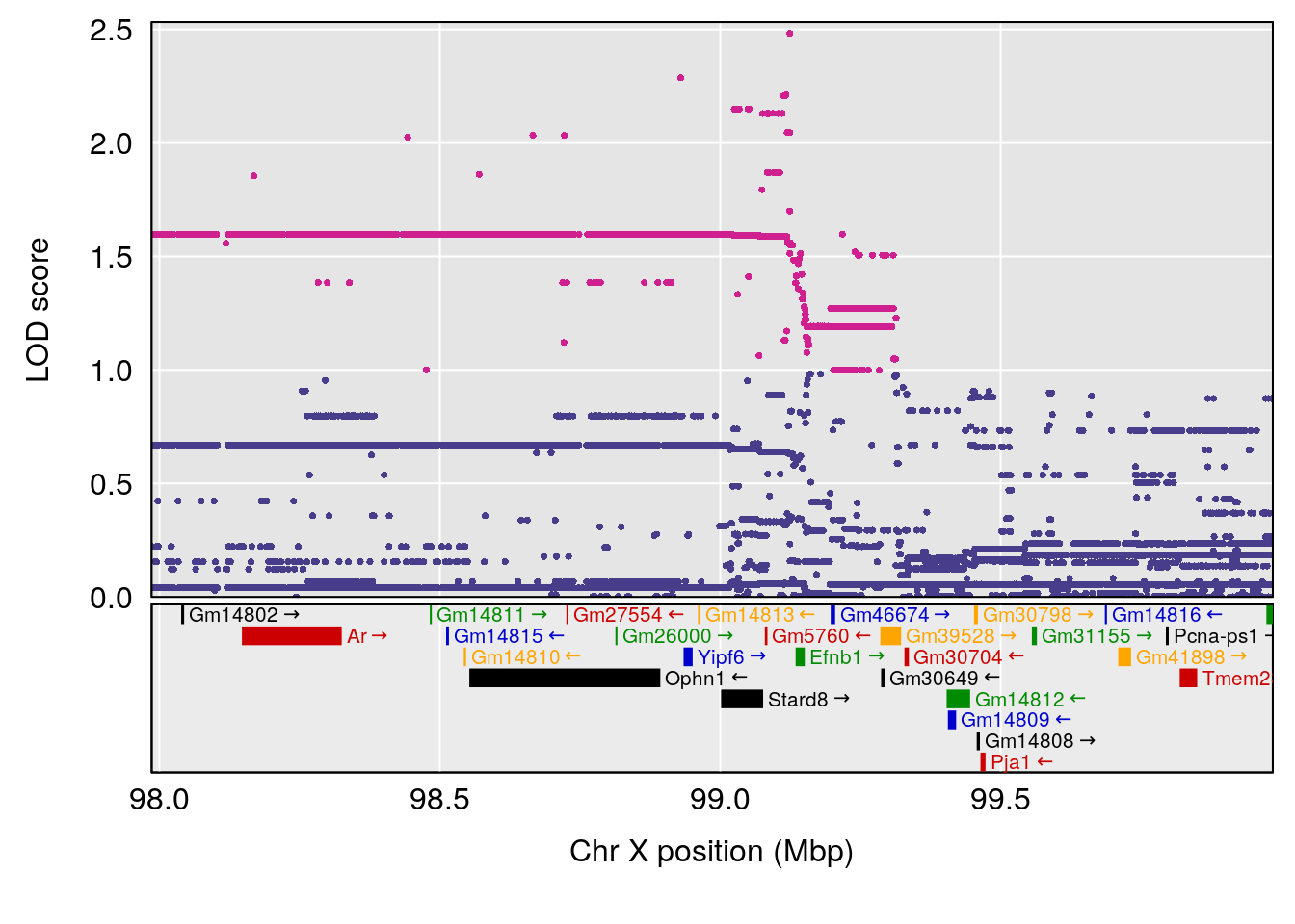
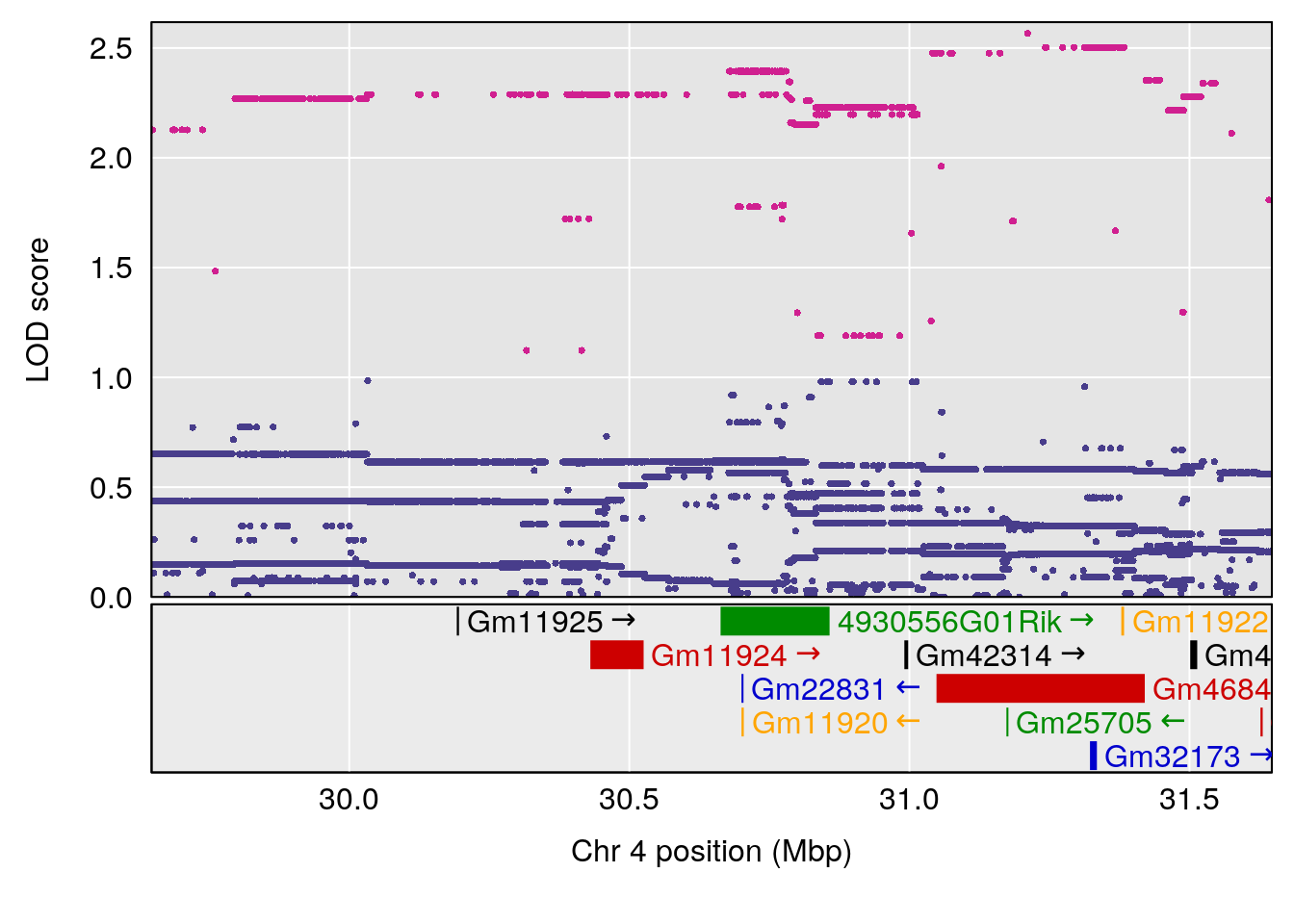
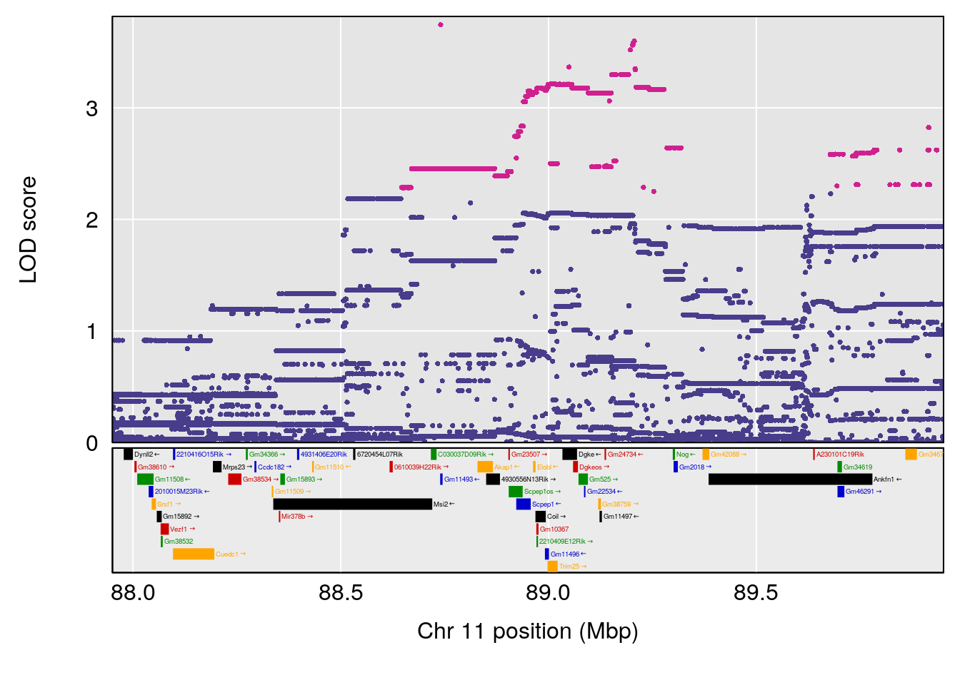
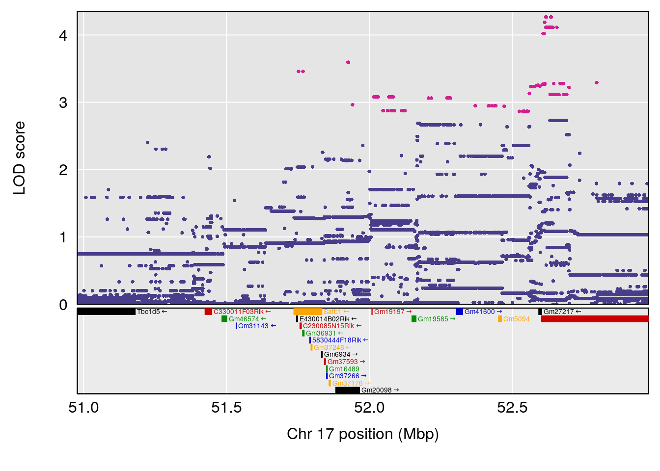
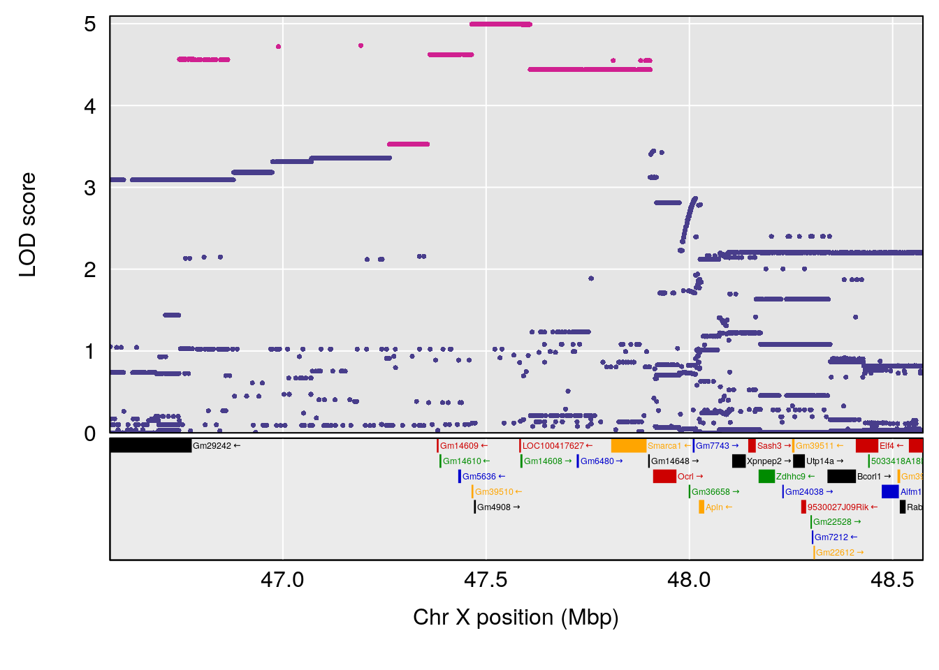
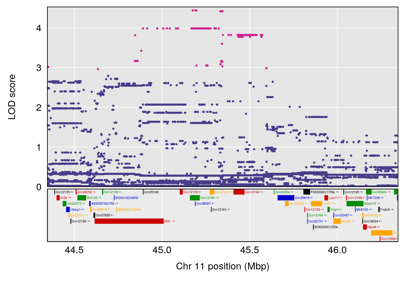
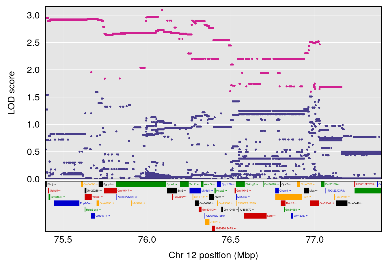
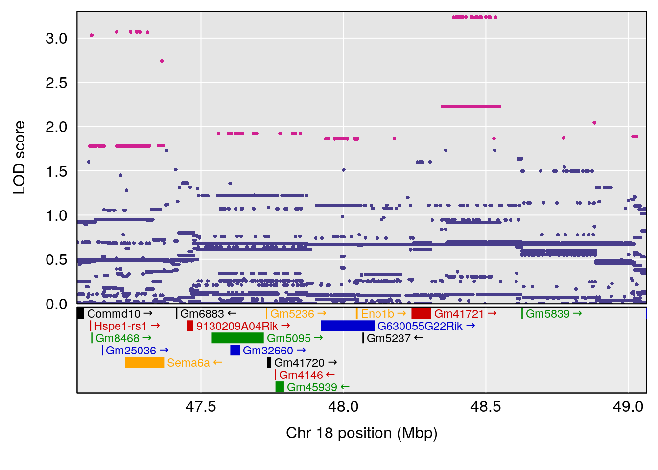
plot(out_snps[[i]][[p]]$lod, out_snps[[i]][[p]]$snpinfo, drop_hilit=1.5, genes=out_genes[[i]][[p]])
}
}
}
# [1] "Survival.Time"
# lodindex lodcolumn chr pos lod ci_lo ci_hi
# 1 1 pheno1 19 35.84901 6.284406 35.4551 37.47958
# [1] 1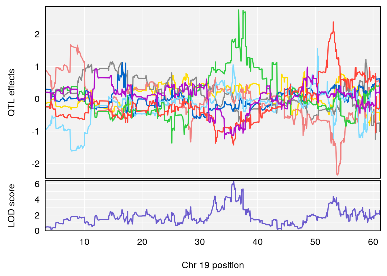
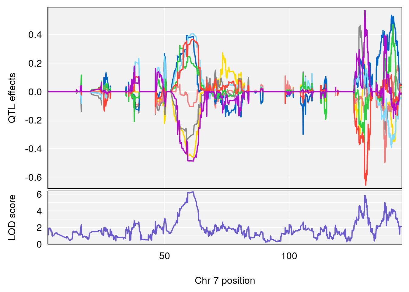
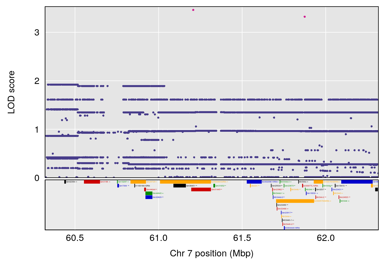
# [1] "Recovery.Time"
# lodindex lodcolumn chr pos lod ci_lo ci_hi
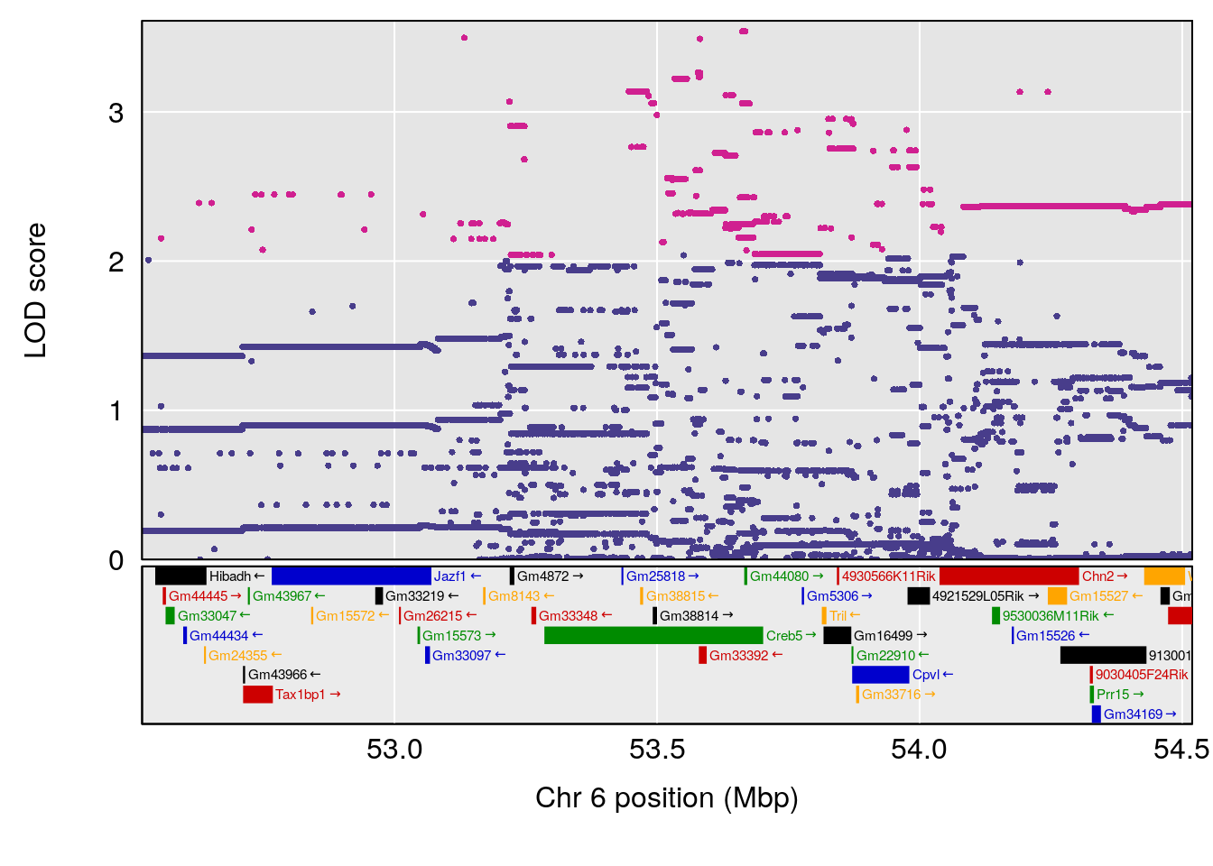
# 1 1 pheno1 6 53.5762 6.455566 53.51503 53.80447
# [1] 1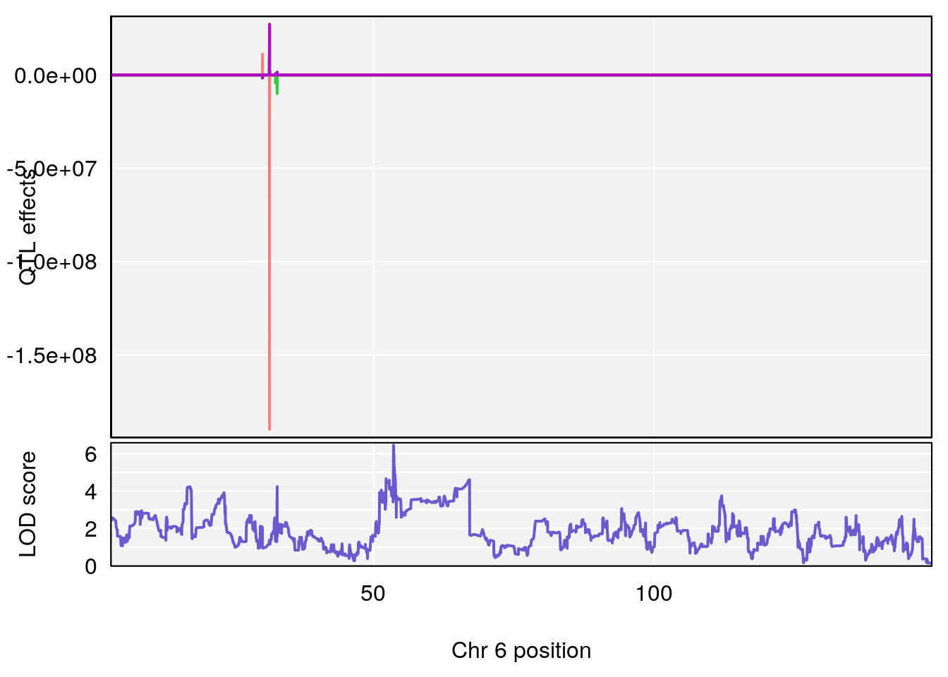
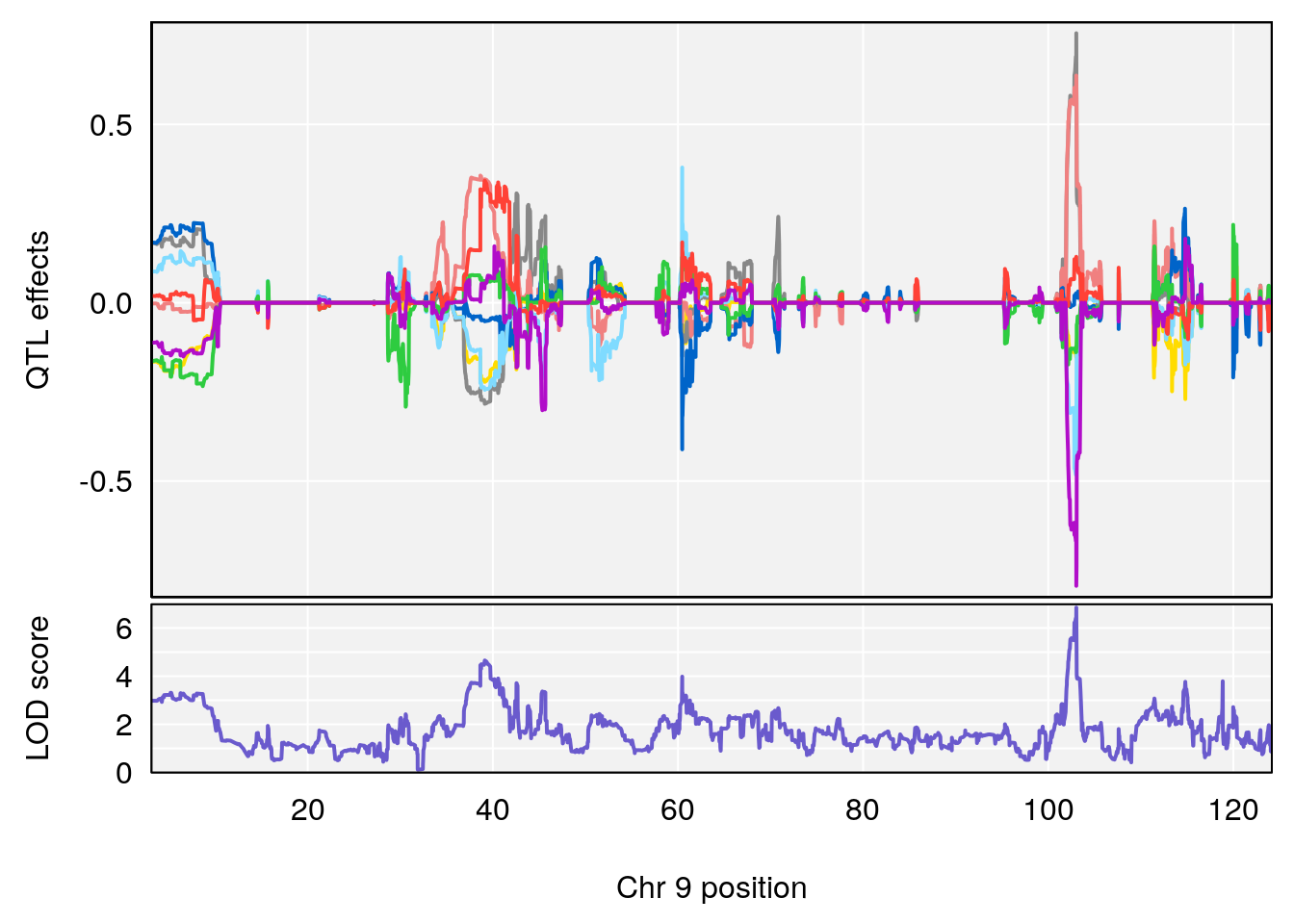
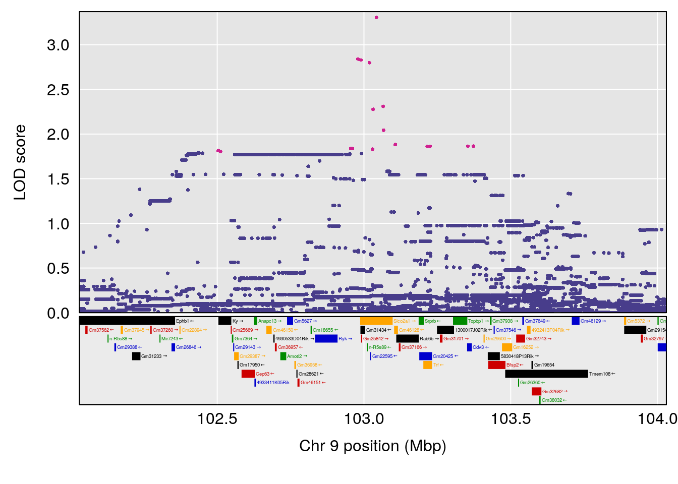
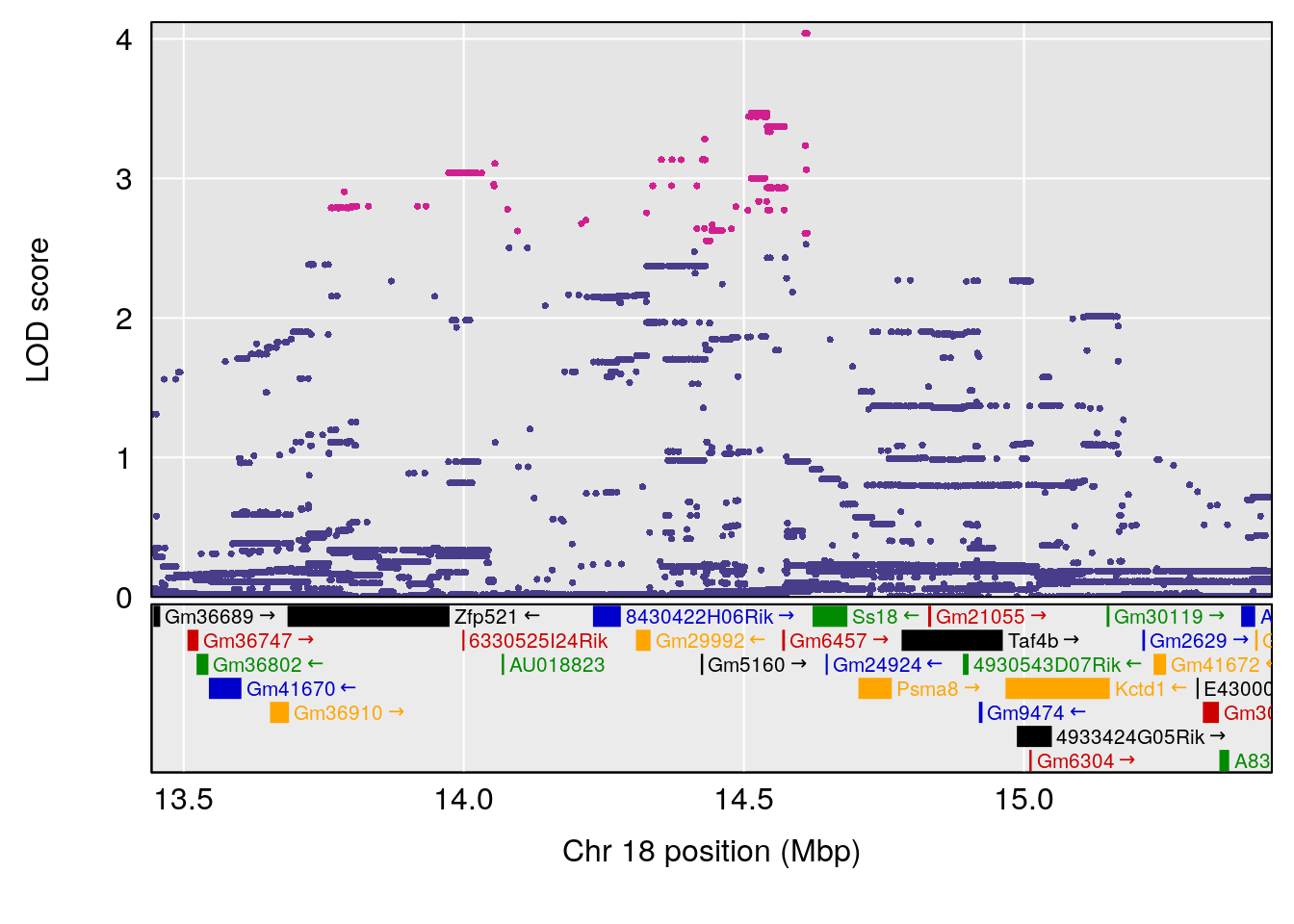
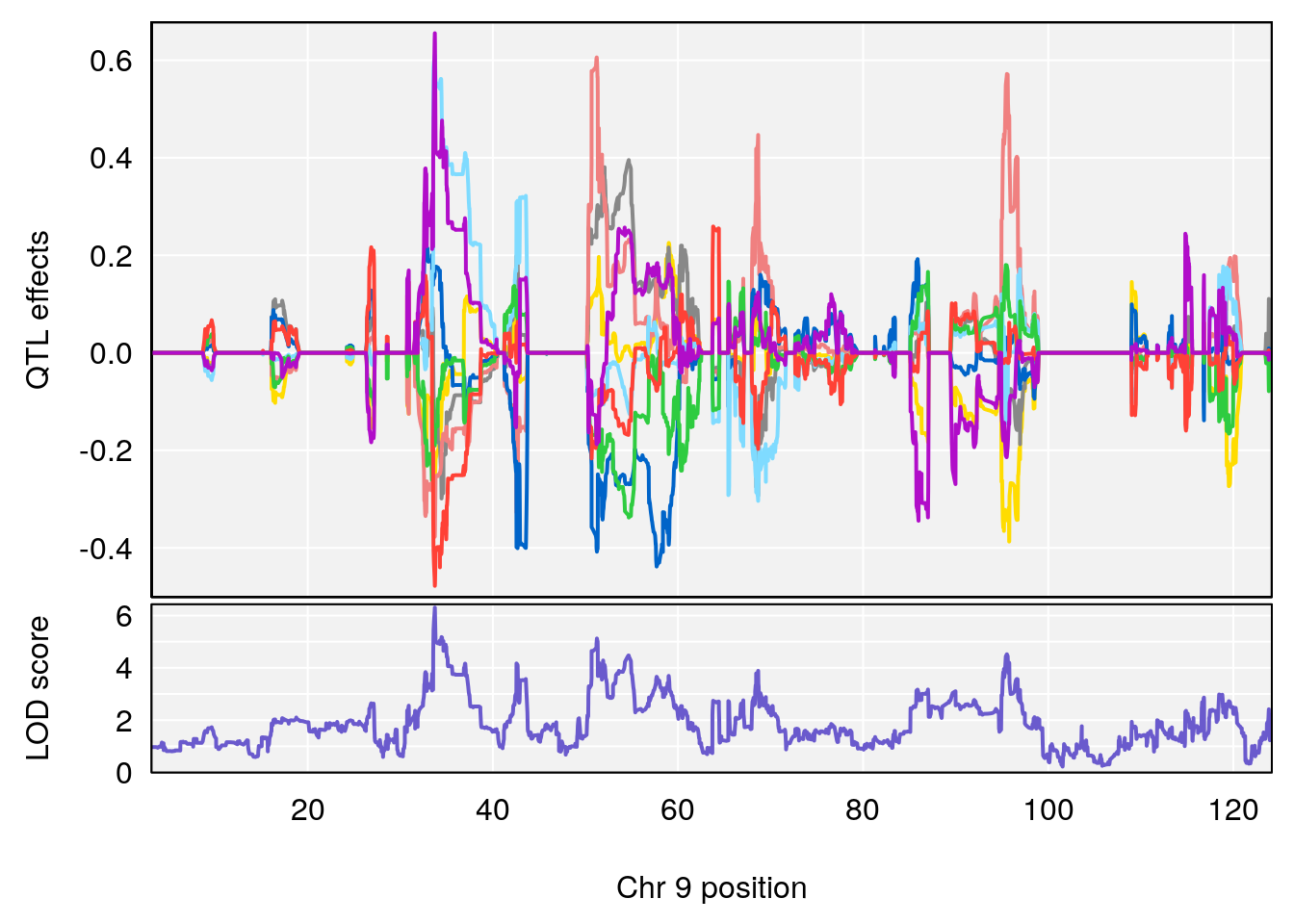
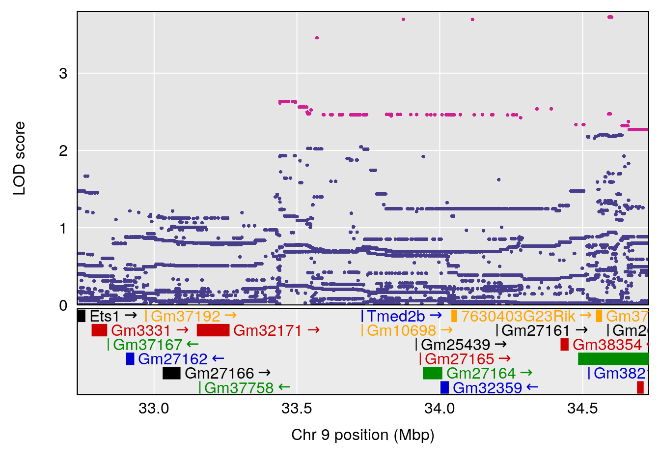
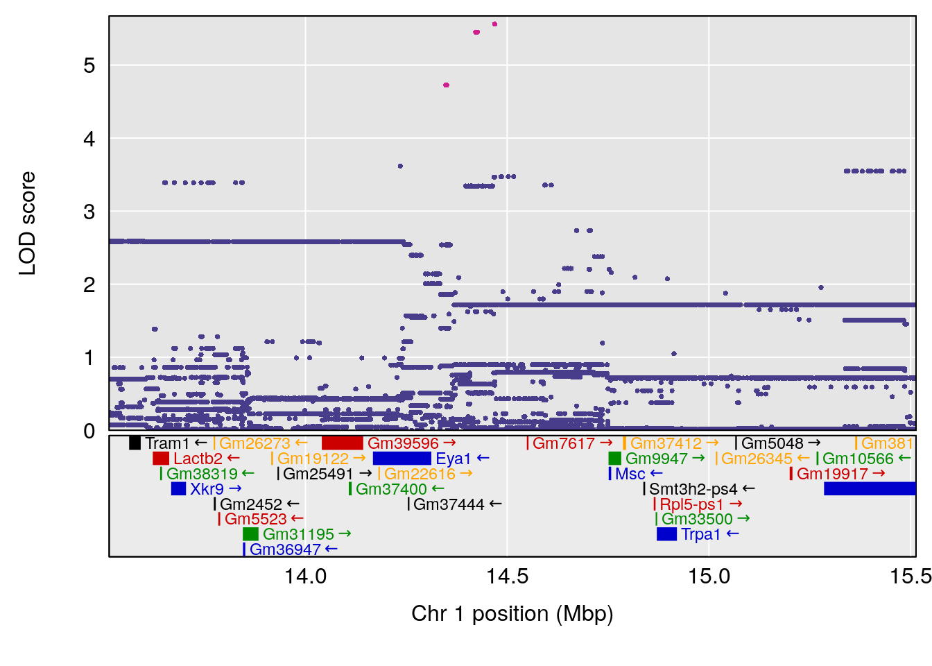
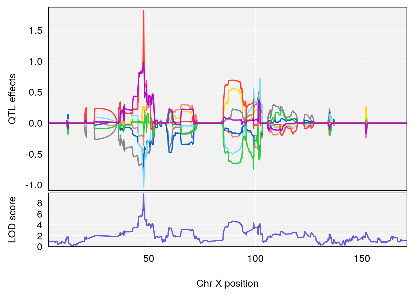
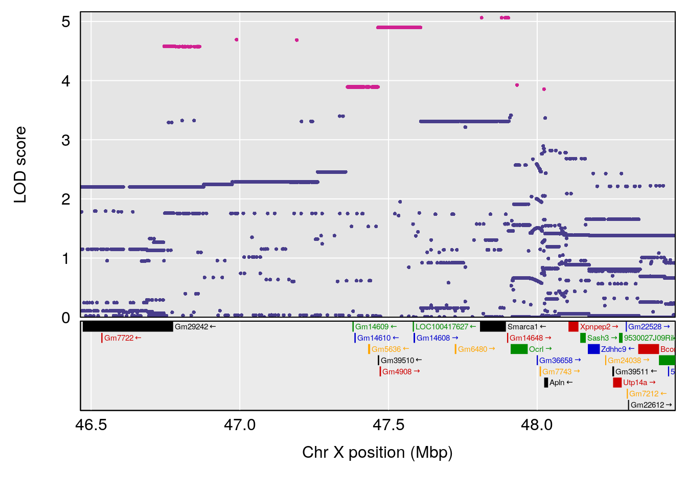
# [1] "Min.depression"
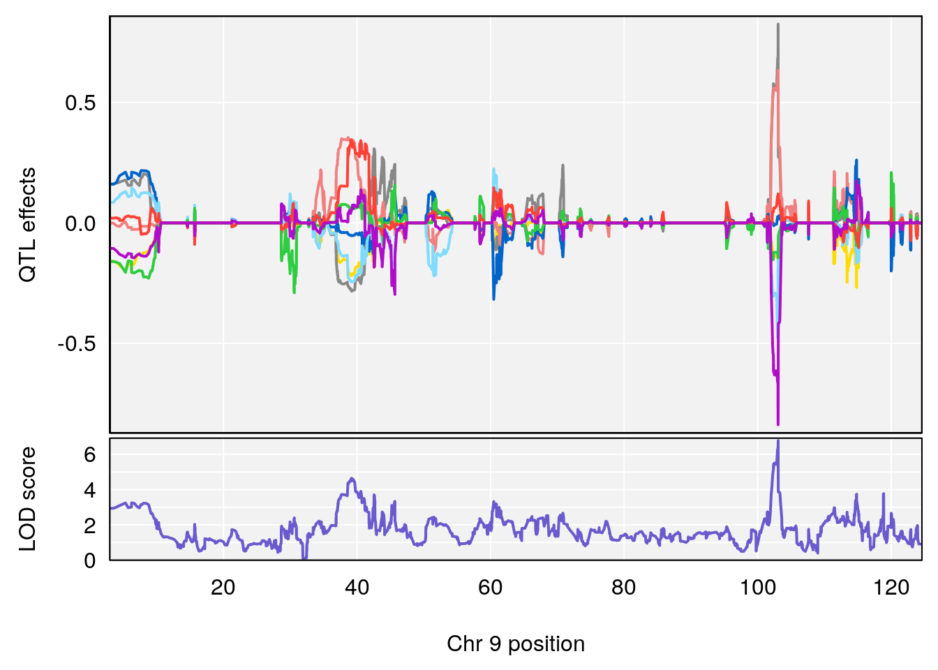
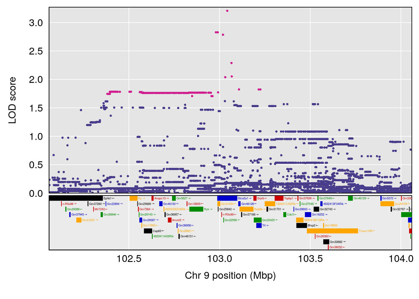
# lodindex lodcolumn chr pos lod ci_lo ci_hi
# 1 1 pheno1 9 103.0304 6.848431 102.3471 103.0599
# [1] 1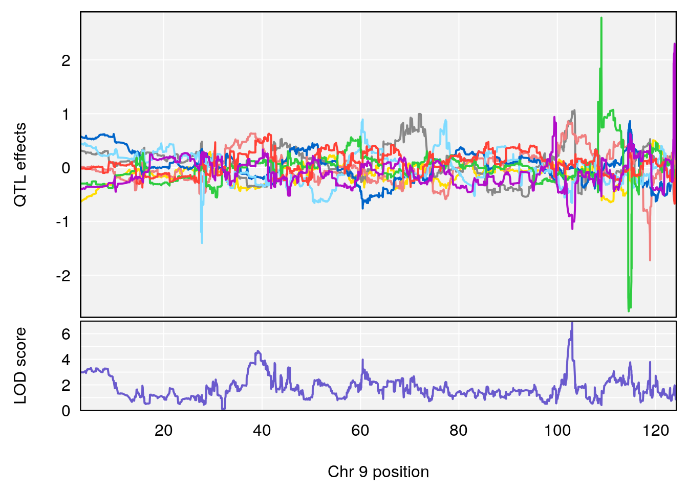
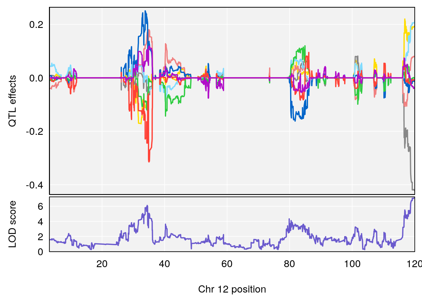
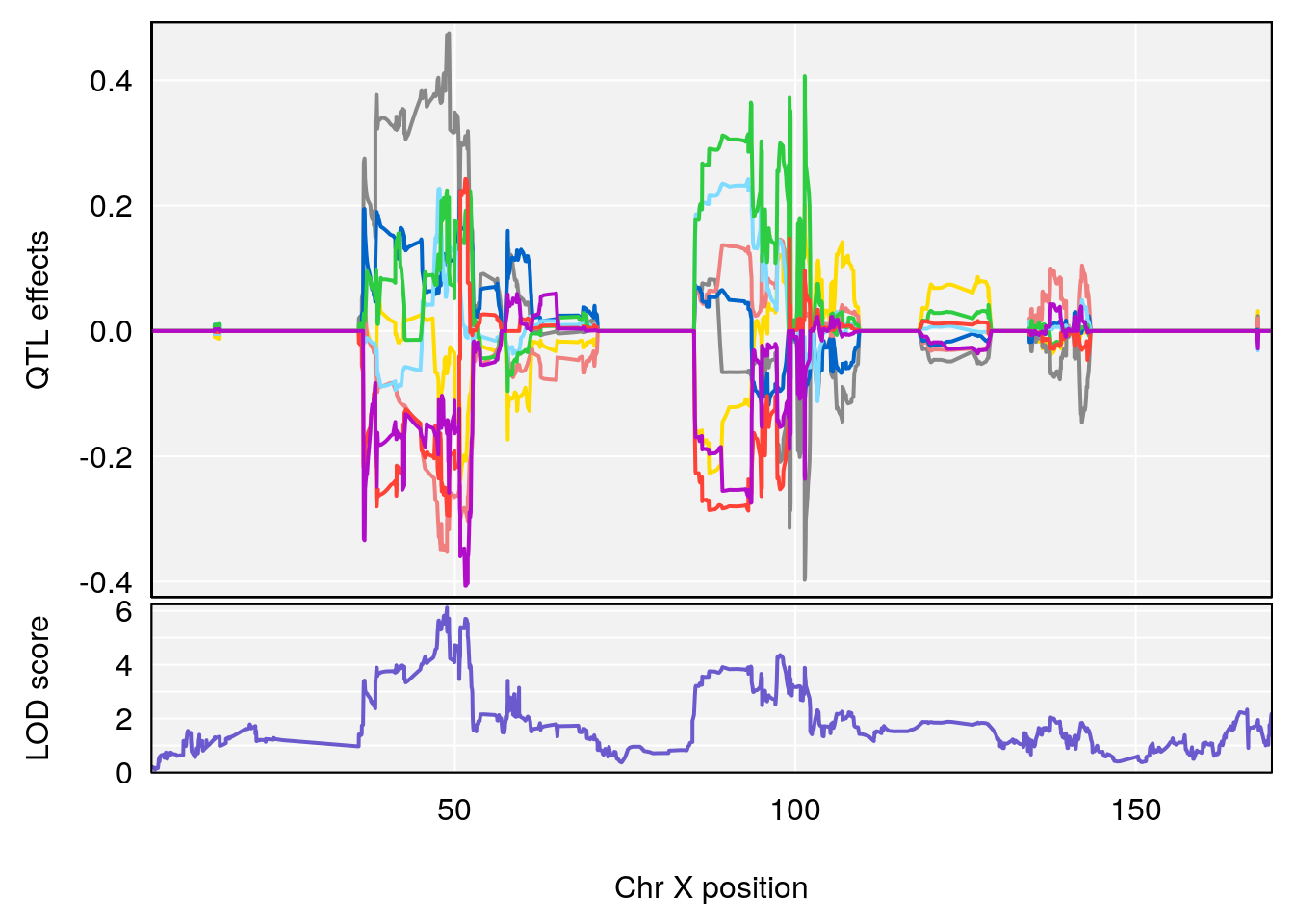
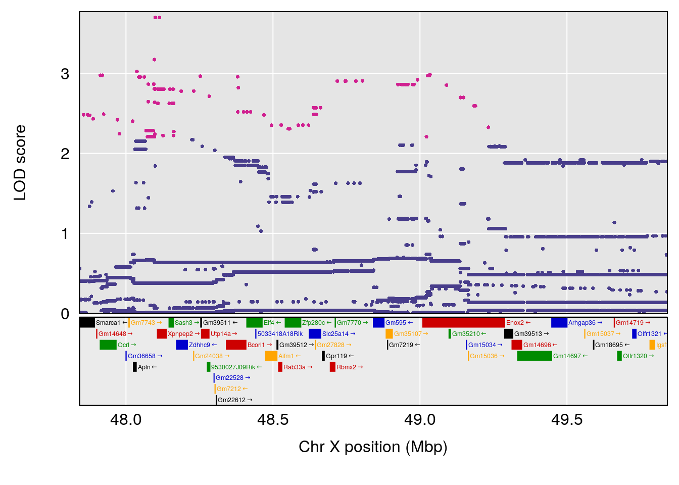
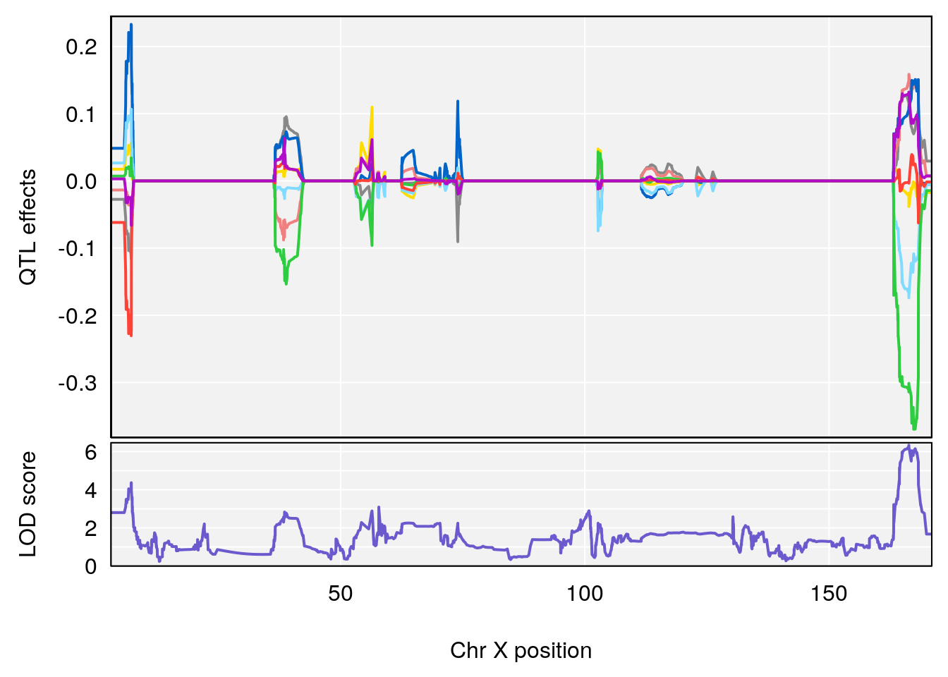
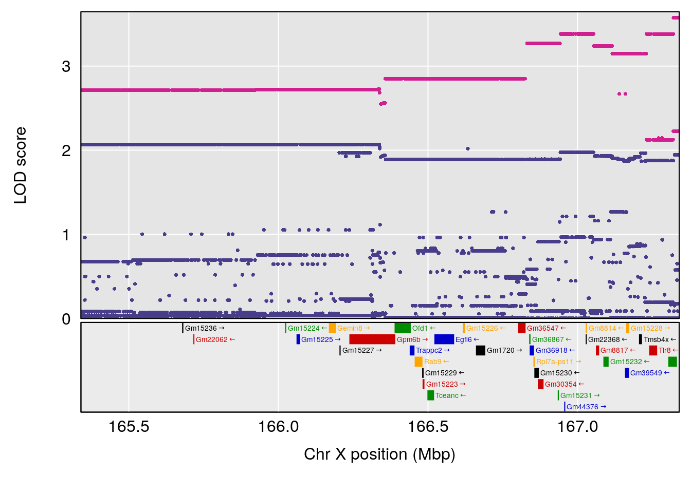
# [1] "Status_bin"
# lodindex lodcolumn chr pos lod ci_lo ci_hi
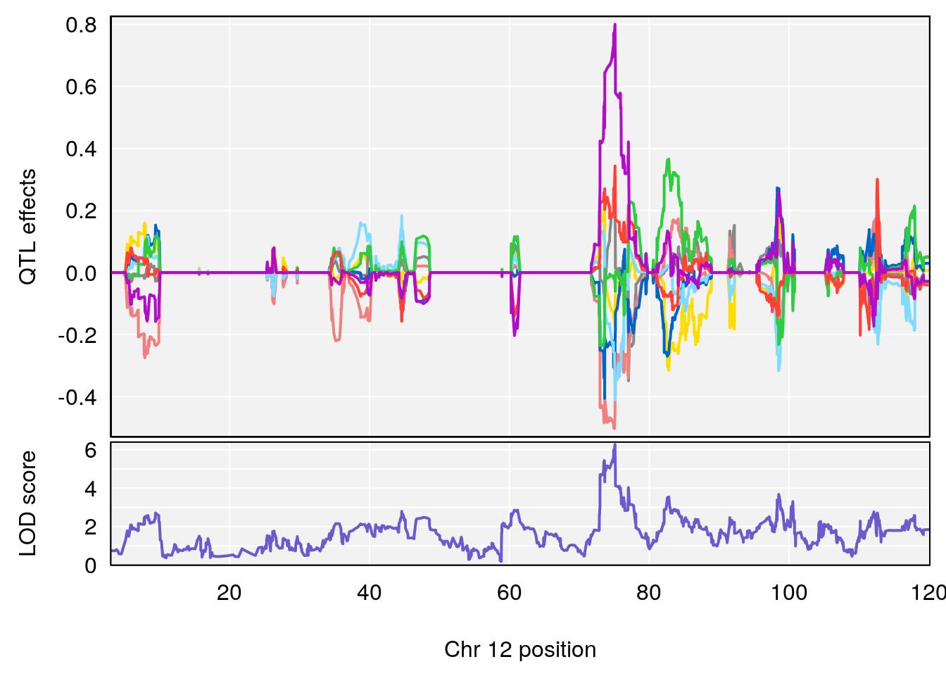
# 1 1 pheno1 12 120.01743 7.098245 33.78237 120.0174
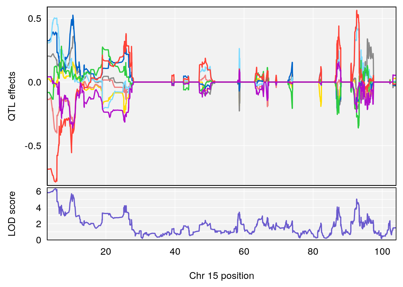
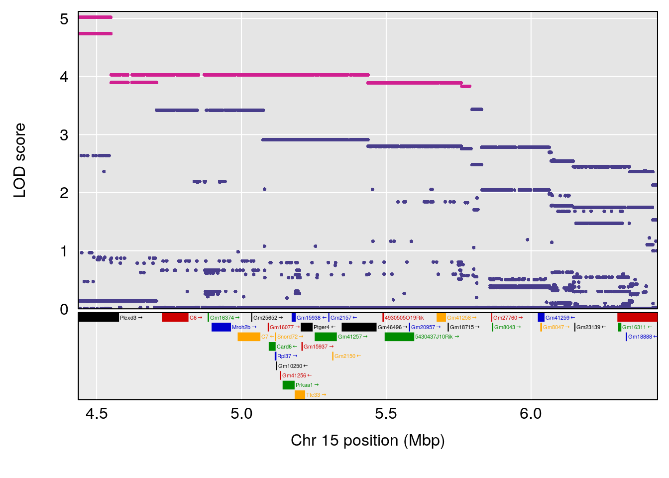
# 2 1 pheno1 15 85.62917 6.063520 51.20007 87.7172
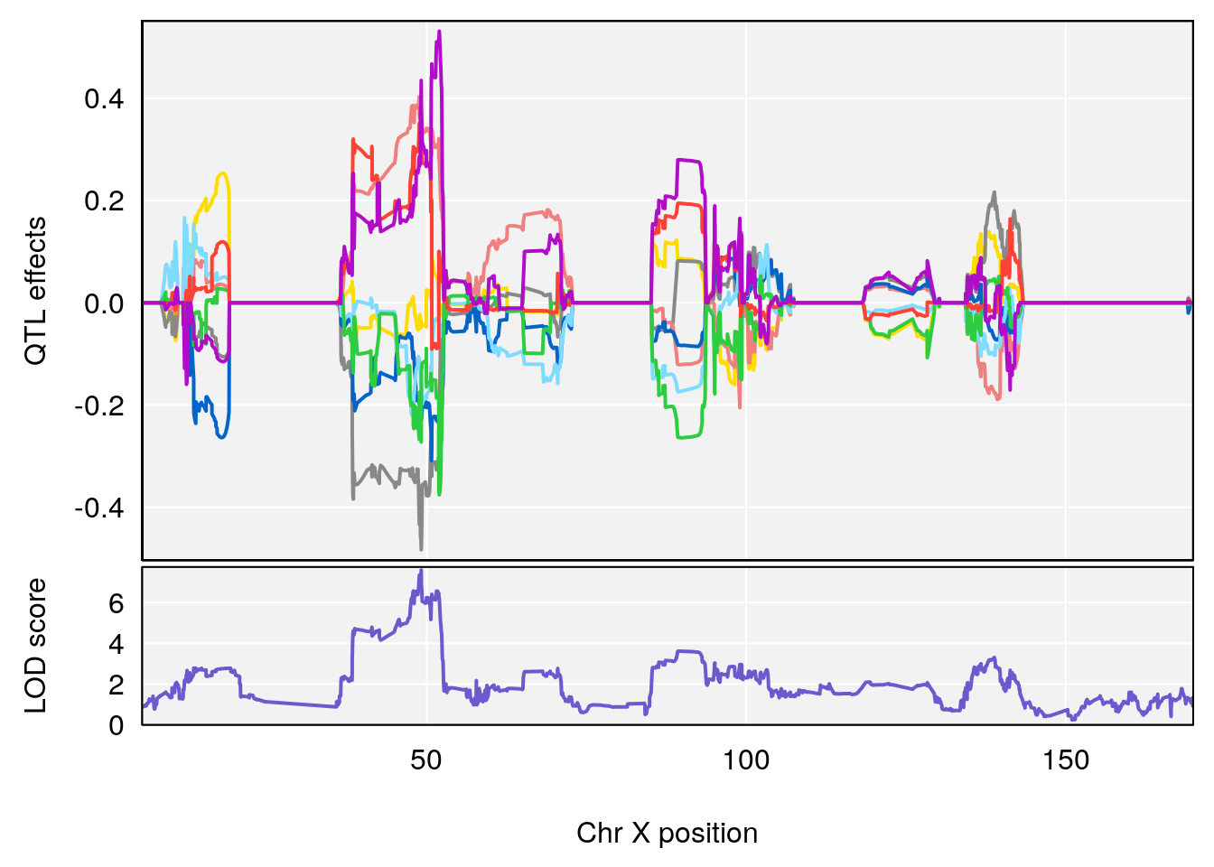
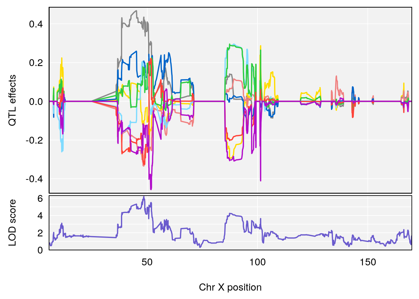
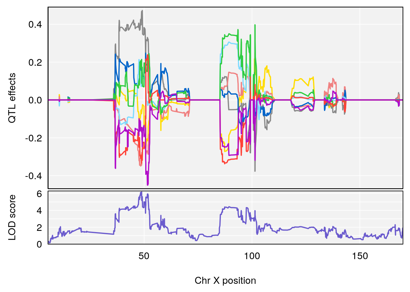
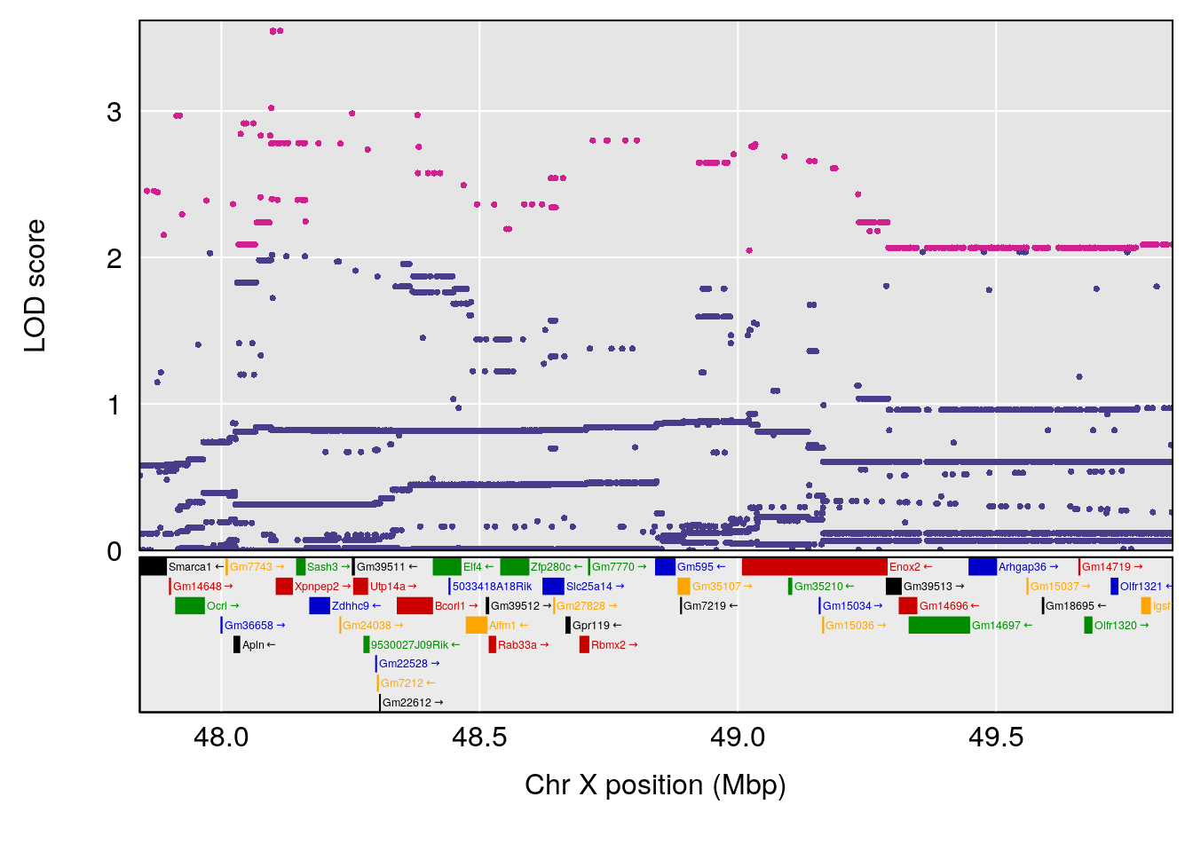
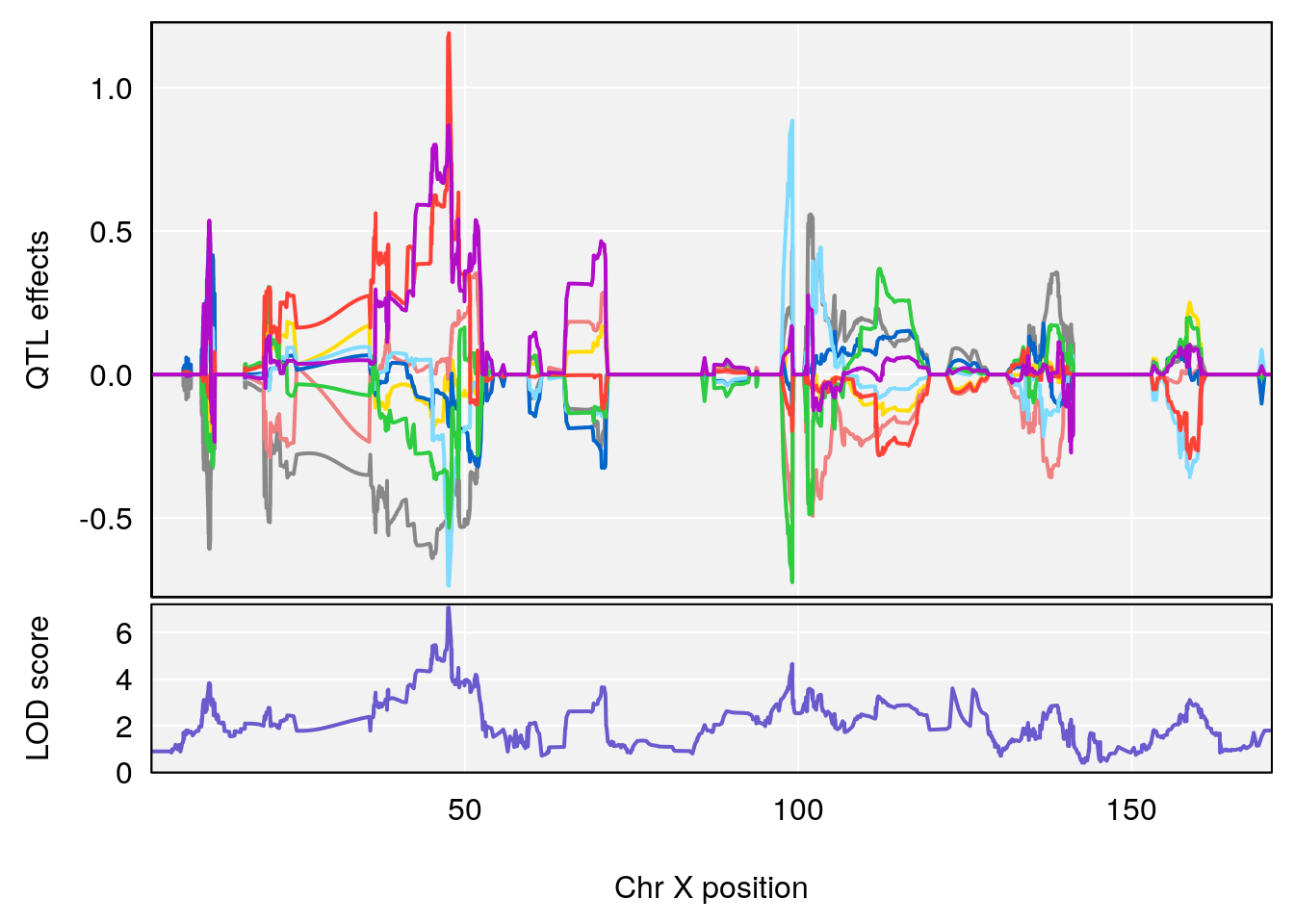
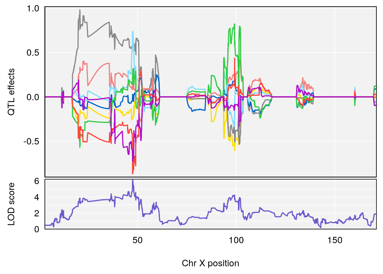
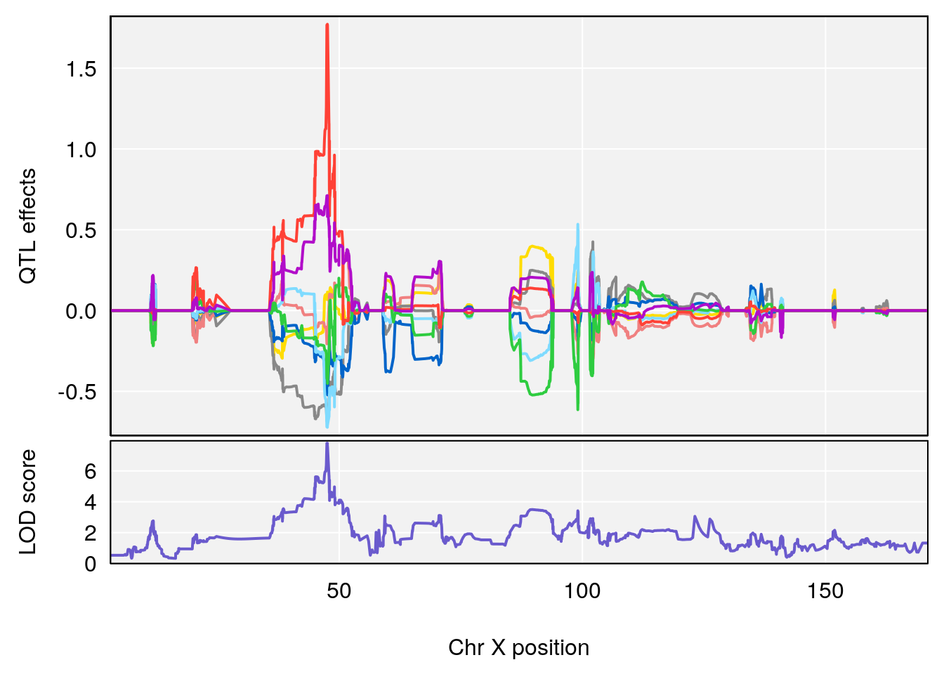
# 3 1 pheno1 X 166.28740 7.992571 163.81034 168.0346
# [1] 1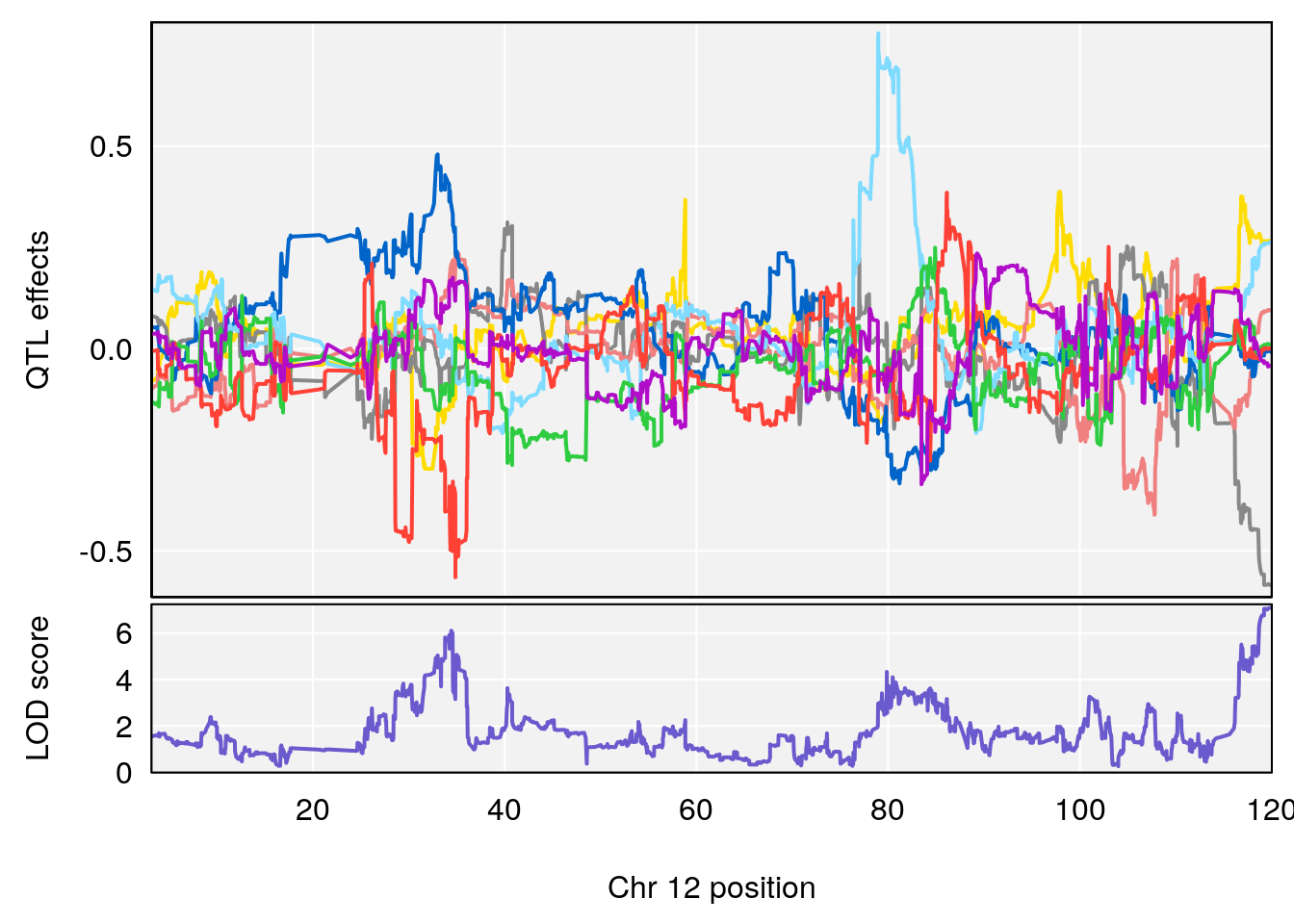
# [1] 2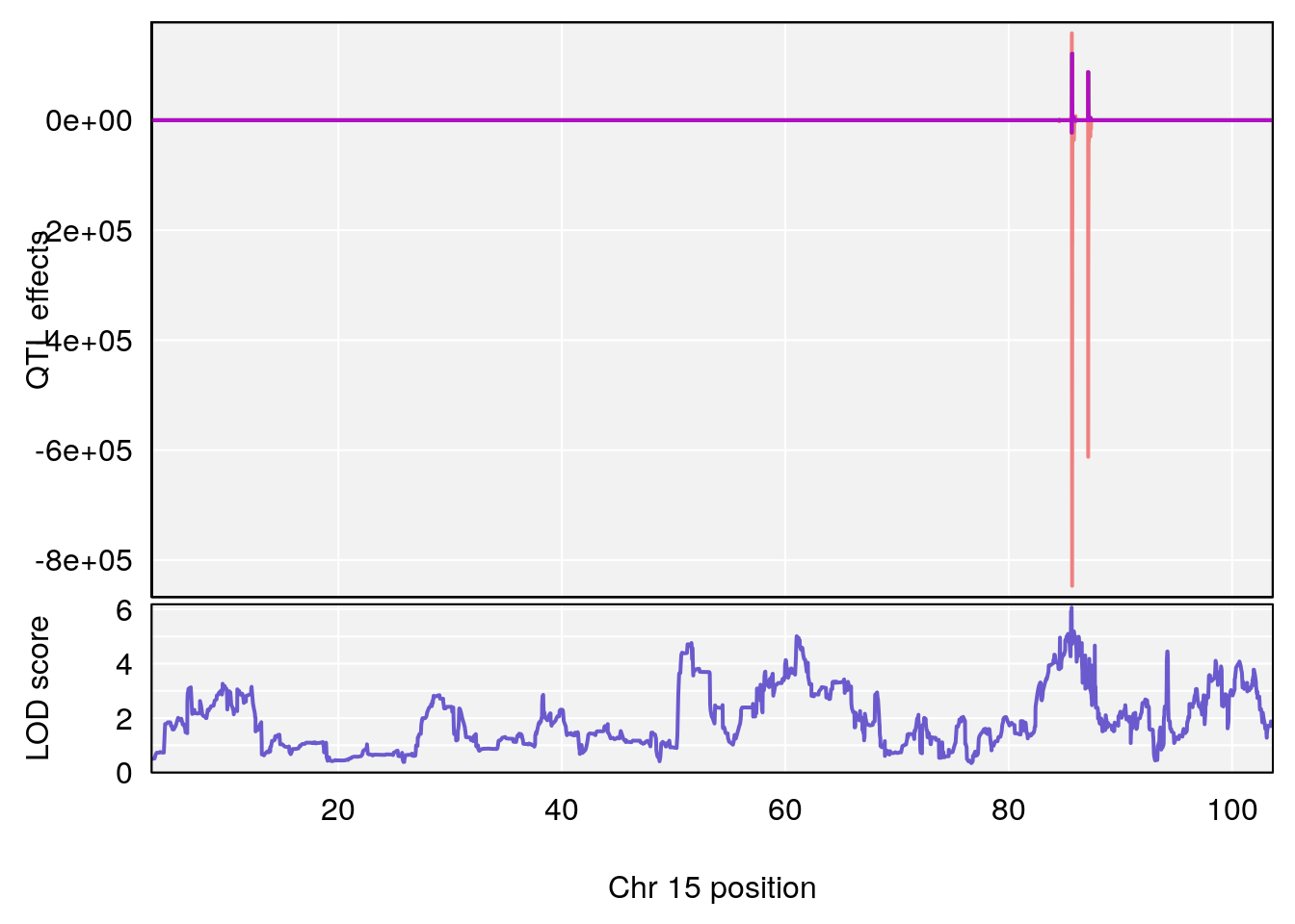

# [1] 3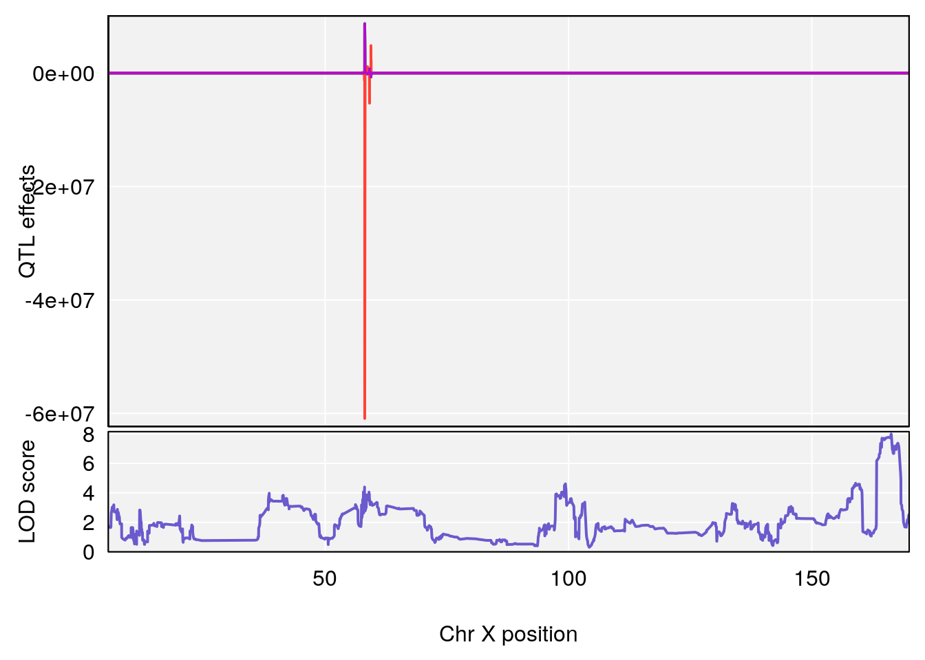
# [1] "f__Bpm"
# lodindex lodcolumn chr pos lod ci_lo ci_hi
# 1 1 pheno1 18 14.44238 6.428647 13.72254 58.39852
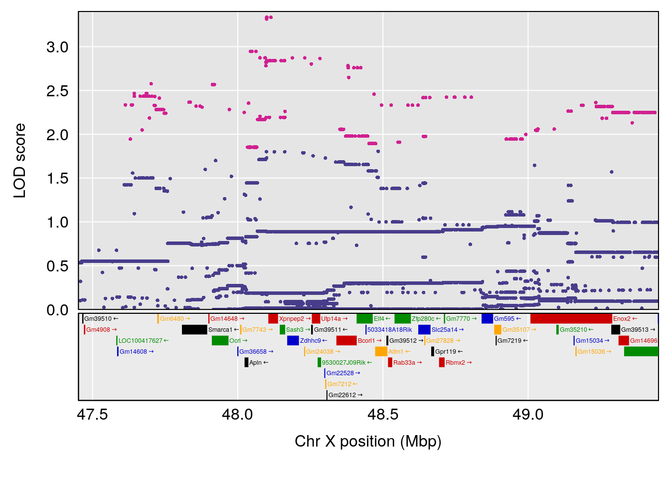
# 2 1 pheno1 X 48.44926 6.964956 47.36754 51.83768
# [1] 1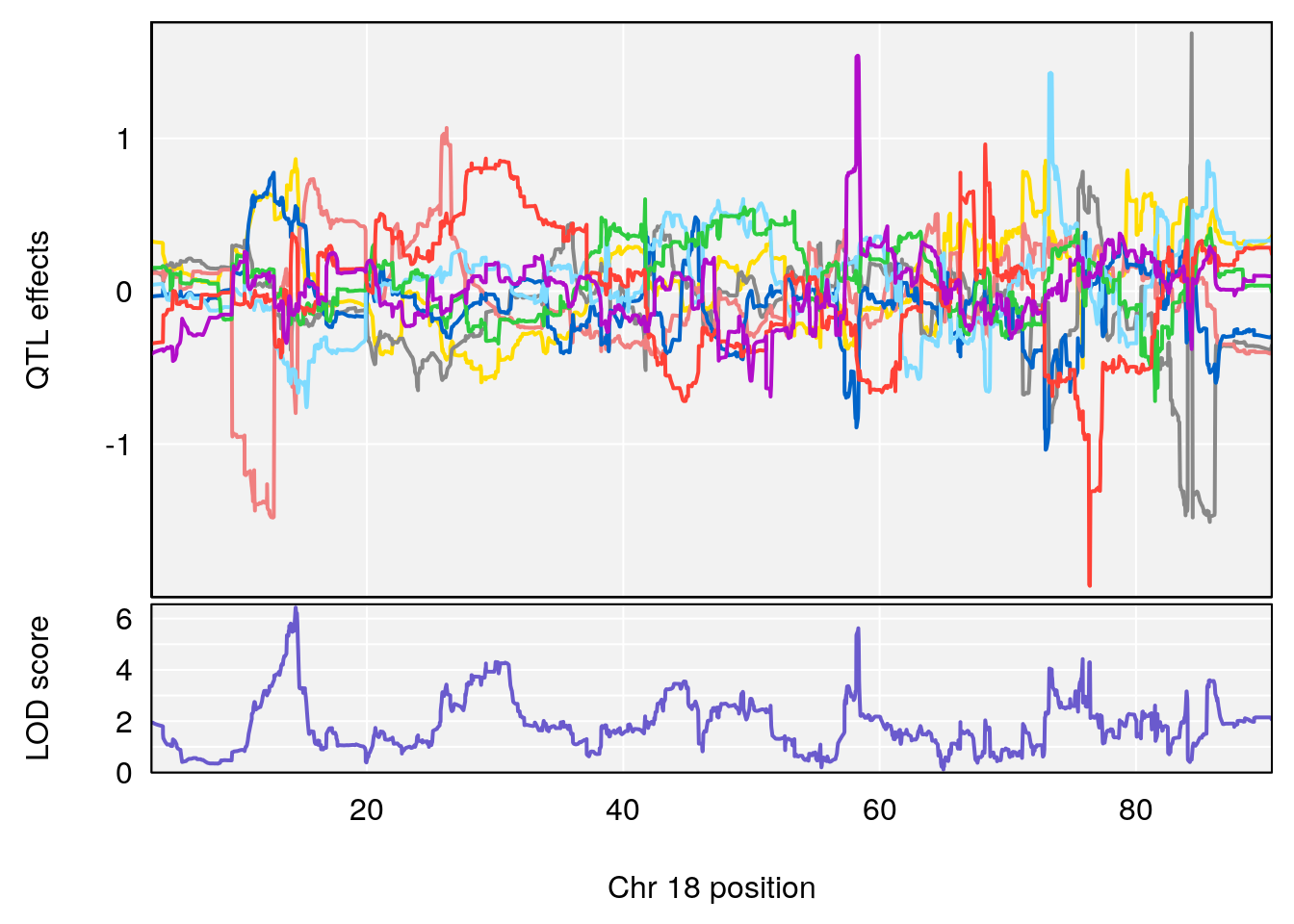
# [1] 2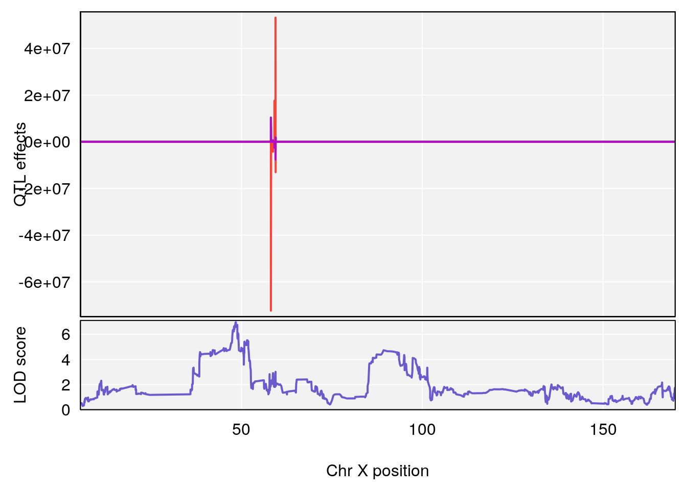
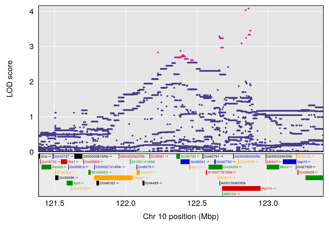
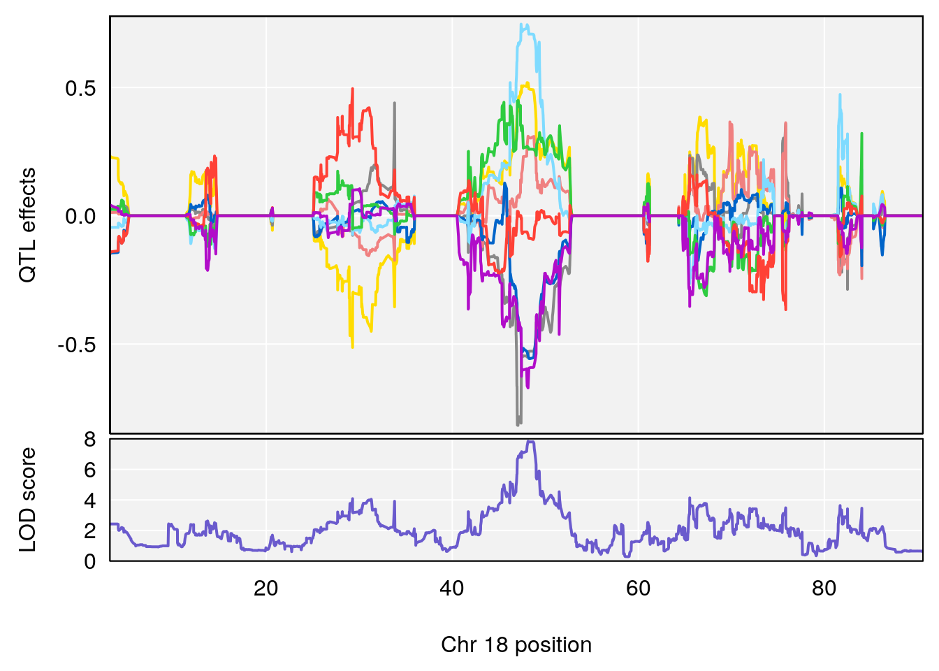
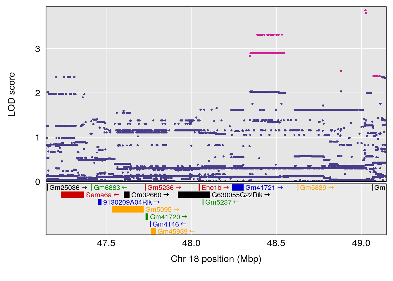
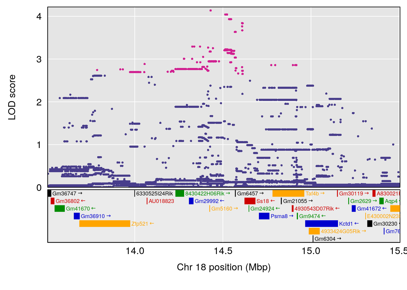
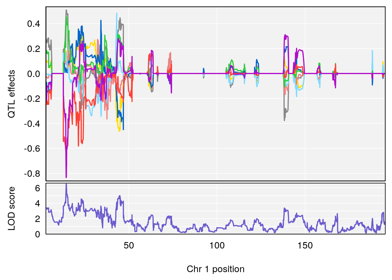
# [1] "TVb_ml"
# lodindex lodcolumn chr pos lod ci_lo ci_hi
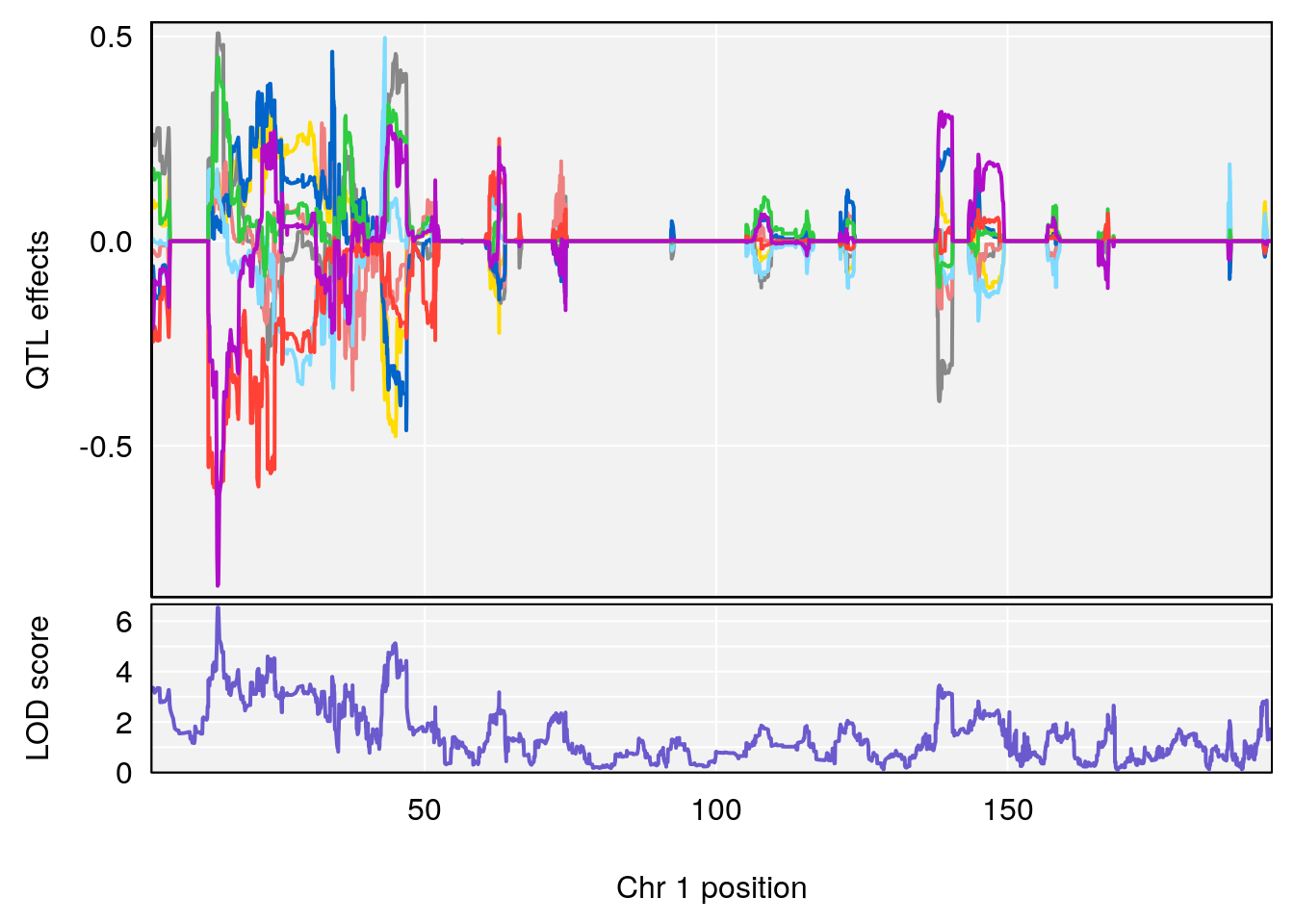
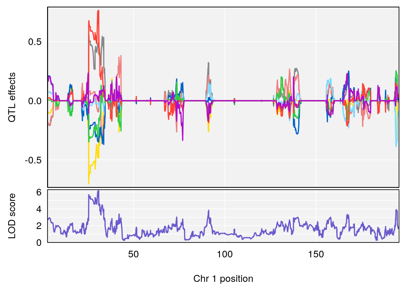
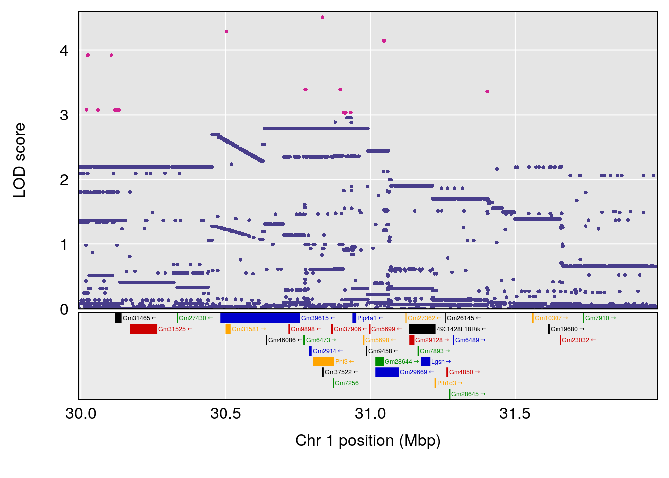
# 1 1 pheno1 1 30.91500 6.091747 25.51861 31.08521
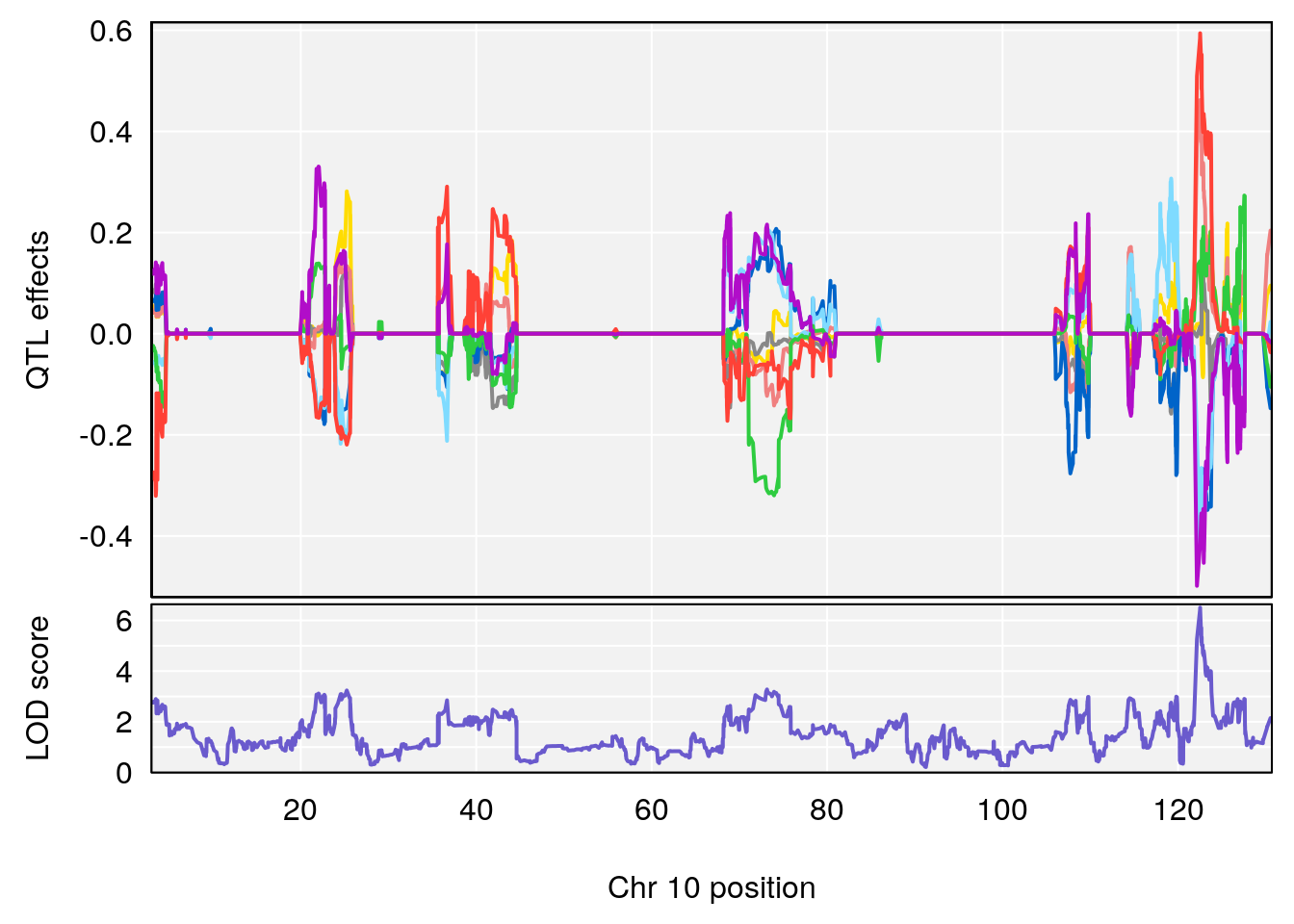
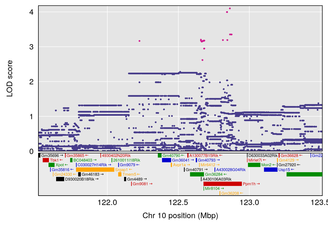
# 2 1 pheno1 10 122.38804 7.251942 122.22638 122.65568
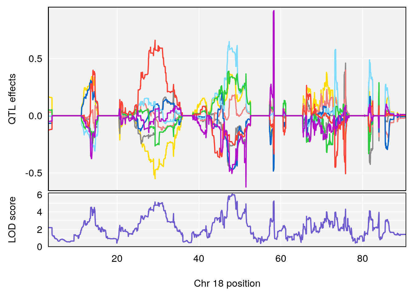
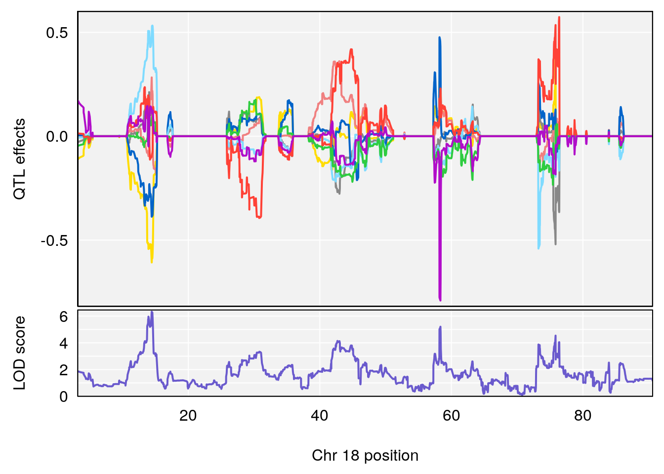
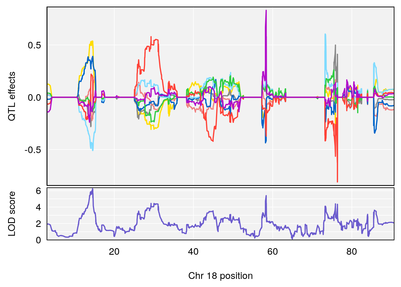
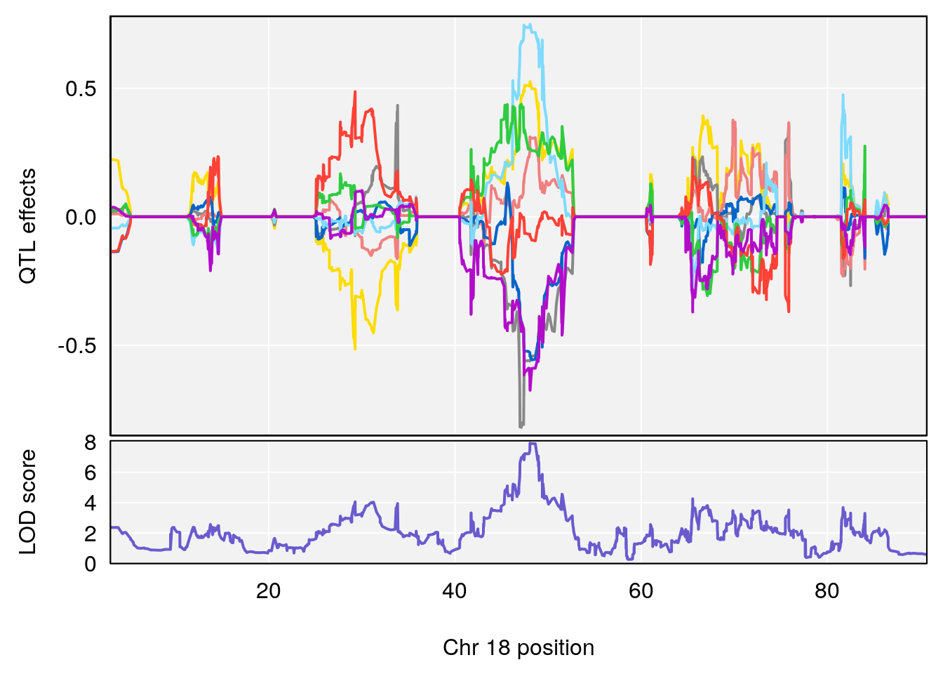
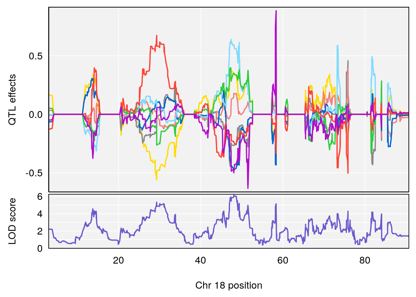
# 3 1 pheno1 18 48.14642 7.848796 46.97402 49.00890
# [1] 1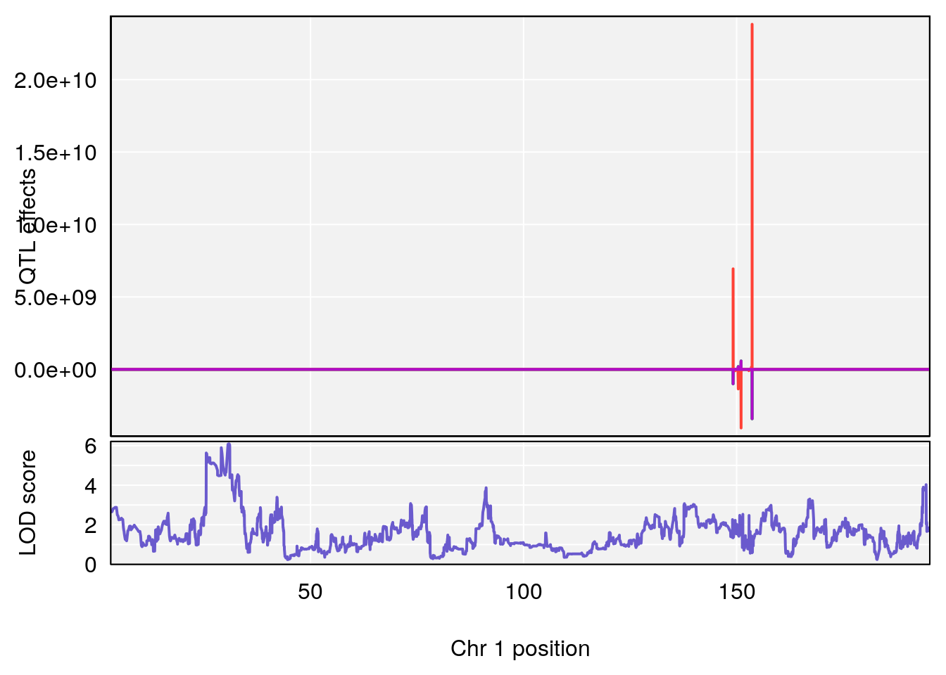
# [1] 2
# [1] 3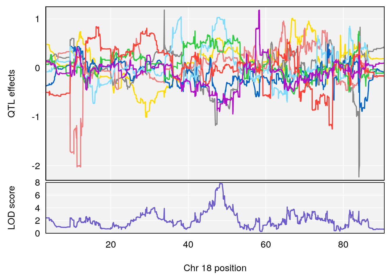
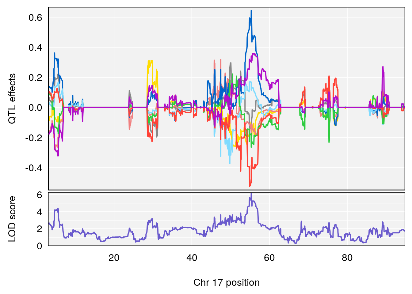
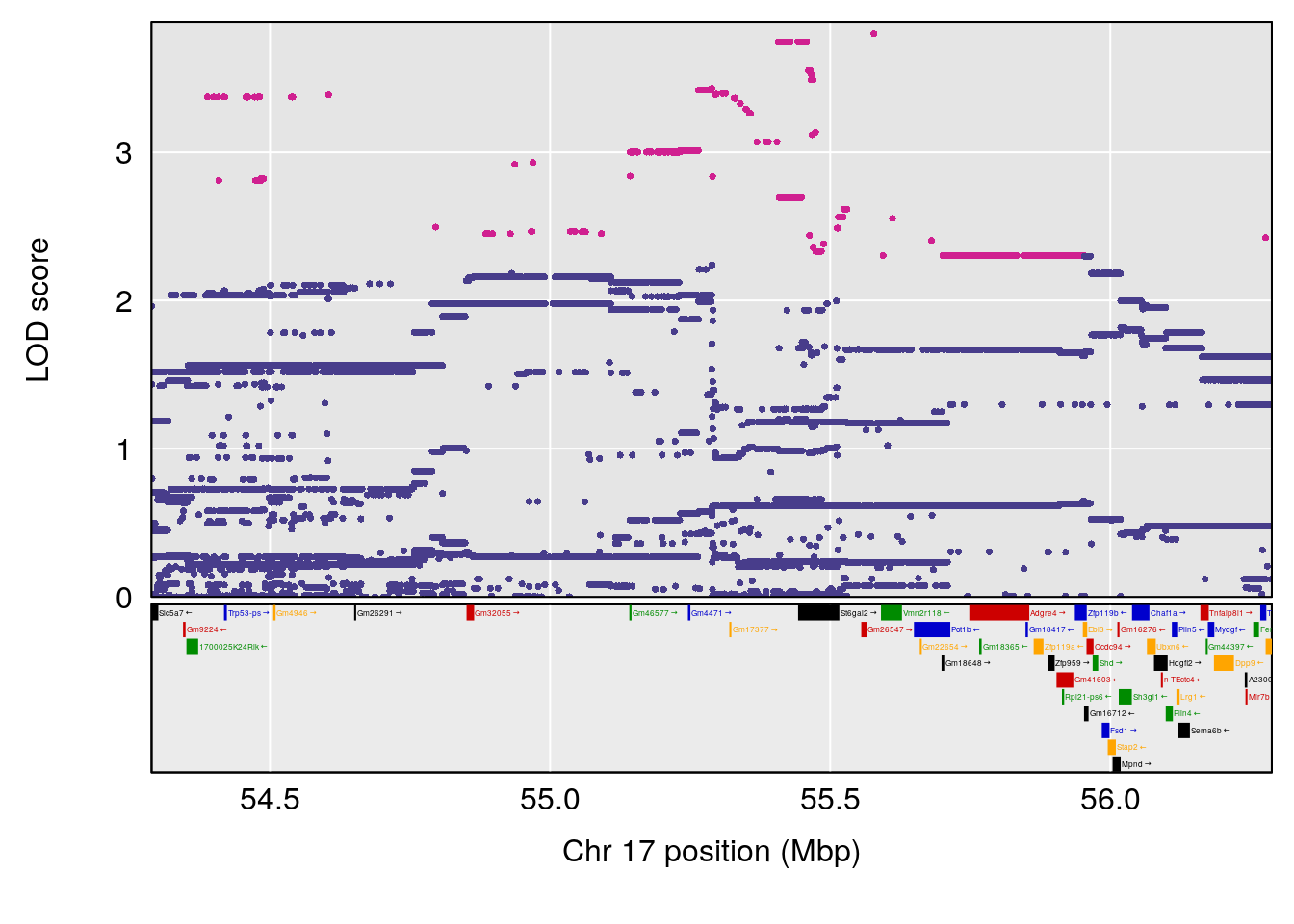
# [1] "MVb__ml_min"
#   lodindex lodcolumn chr      pos      lod    ci_lo    ci_hi
# 1        1    pheno1  17 55.28827 6.148429 54.75322 56.49849
# [1] 1
# [1] "Penh"
# lodindex lodcolumn chr pos lod ci_lo ci_hi
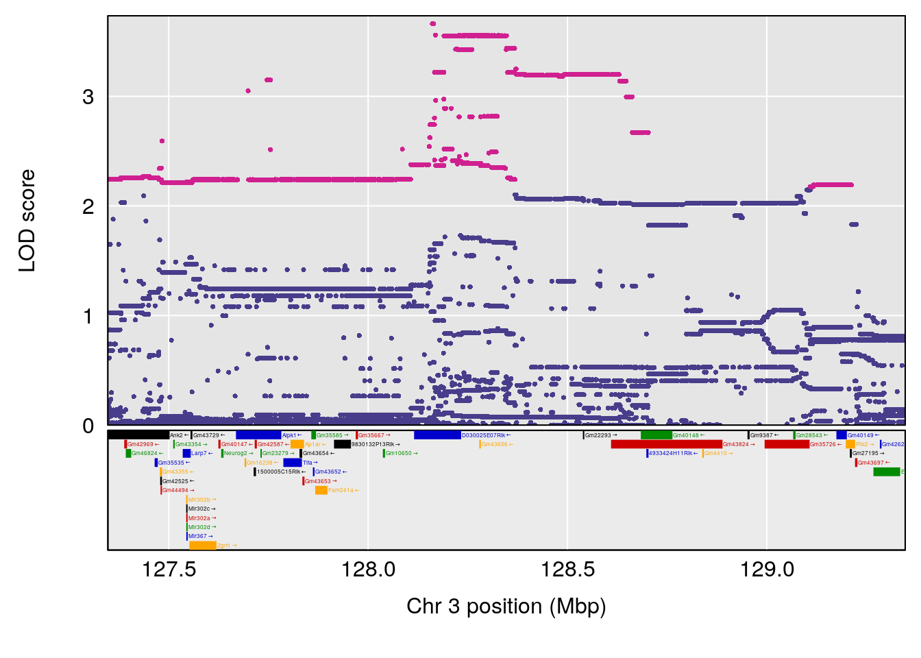
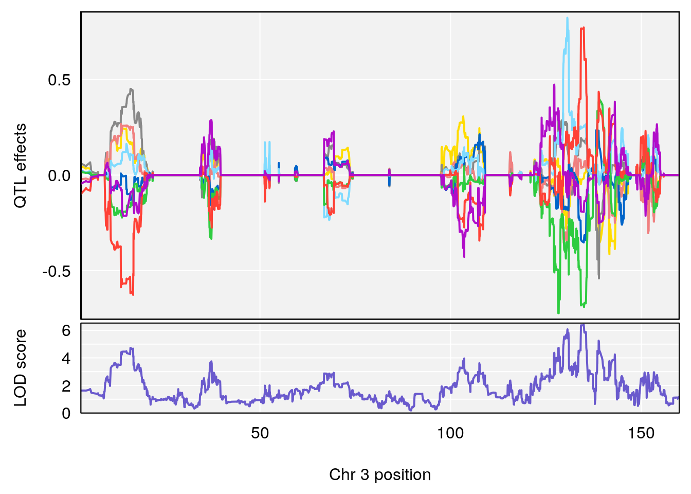
# 1 1 pheno1 3 128.34723 6.070258 103.19697 139.22754
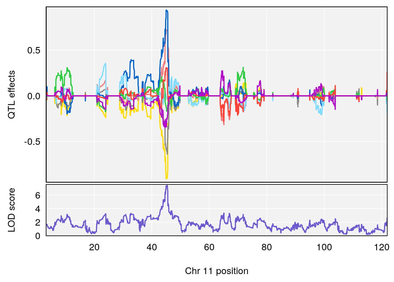
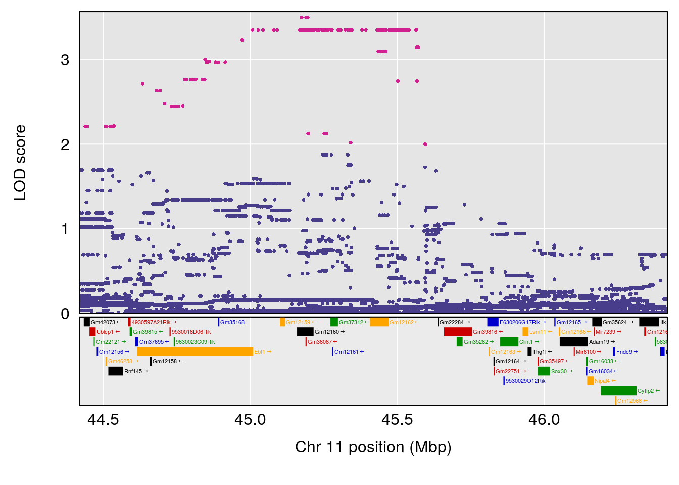
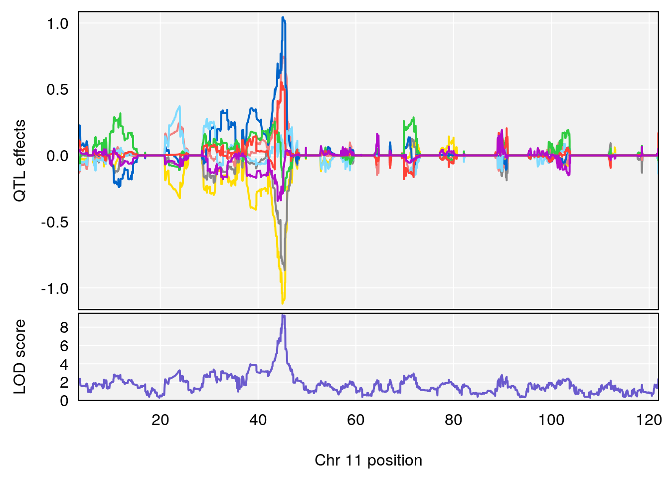
# 2 1 pheno1 11 45.41904 7.430101 44.59625 45.59516
# [1] 1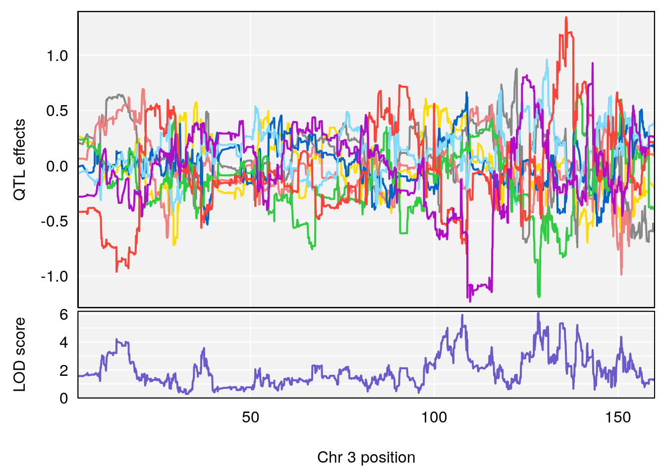
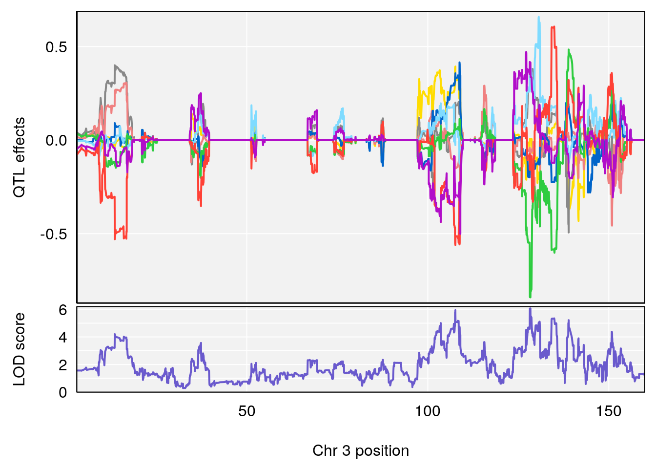
# [1] 2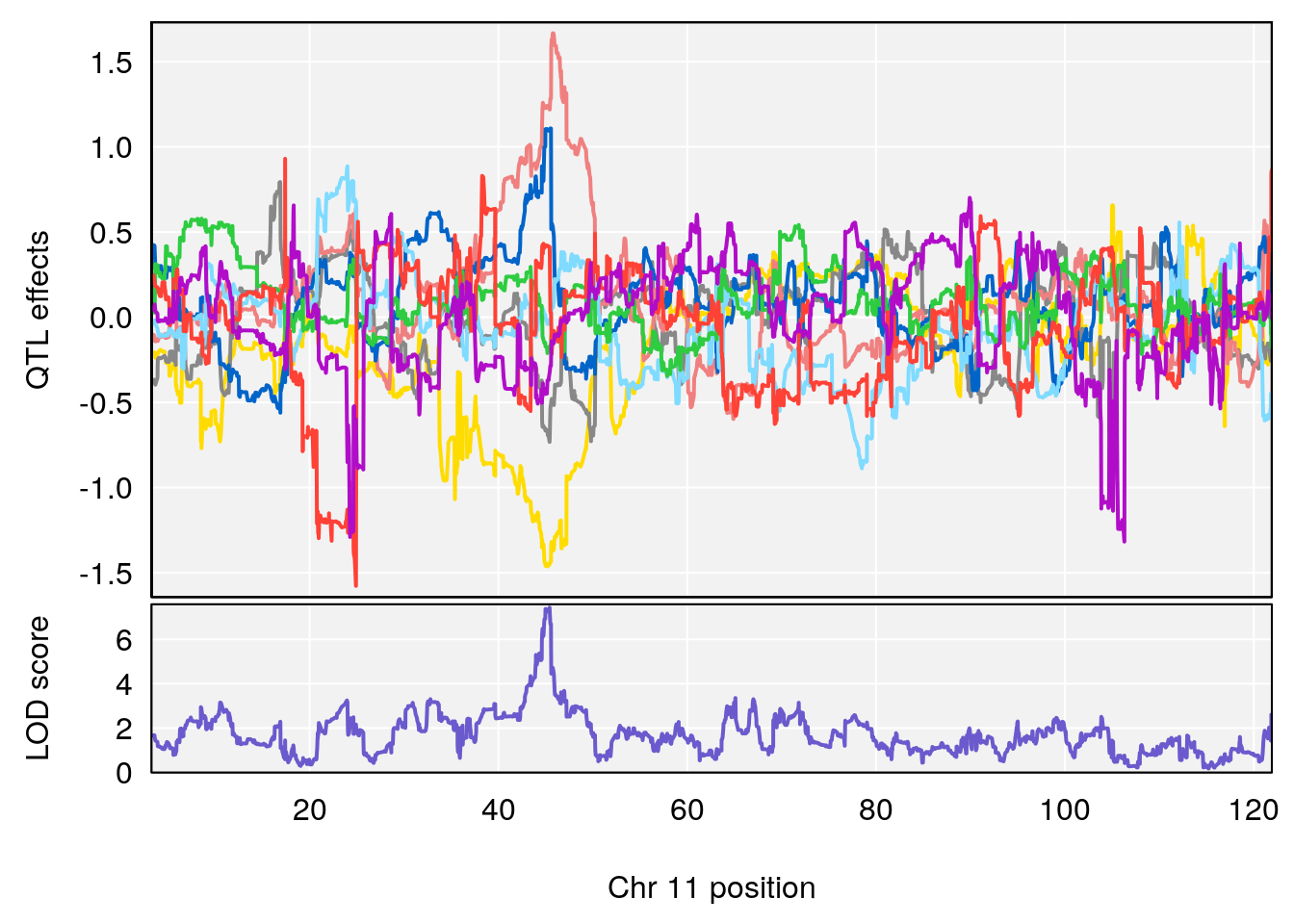
# [1] "PAU"
# lodindex lodcolumn chr pos lod ci_lo ci_hi
# 1 1 pheno1 2 50.65302 6.027406 17.79371 65.30586
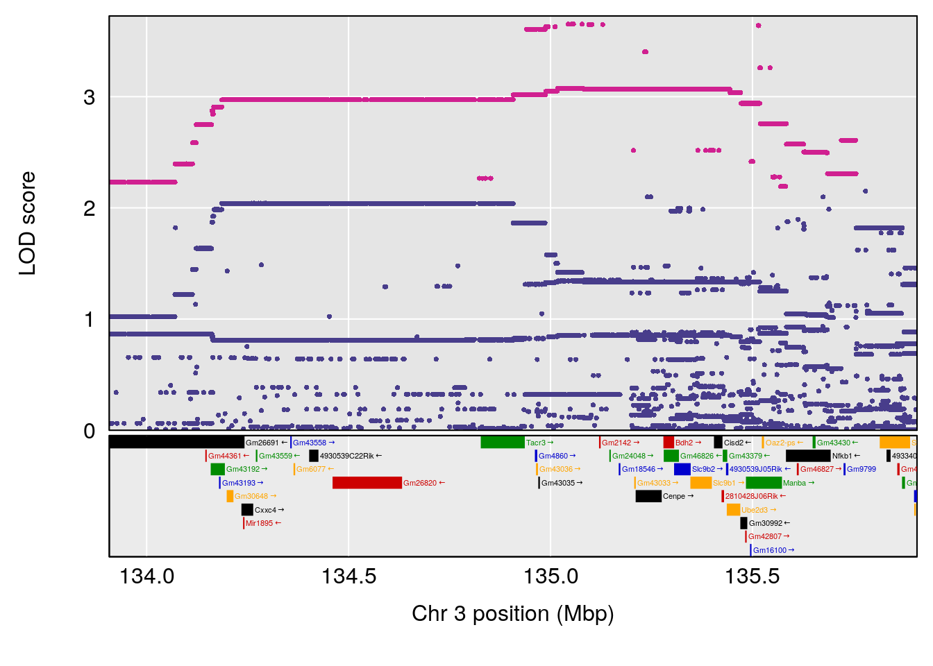
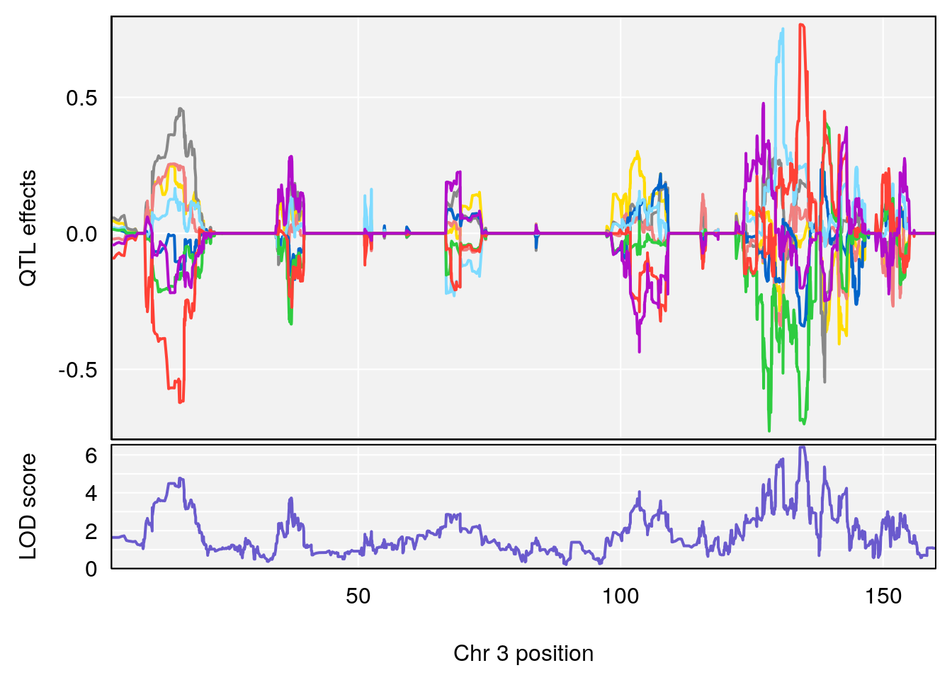
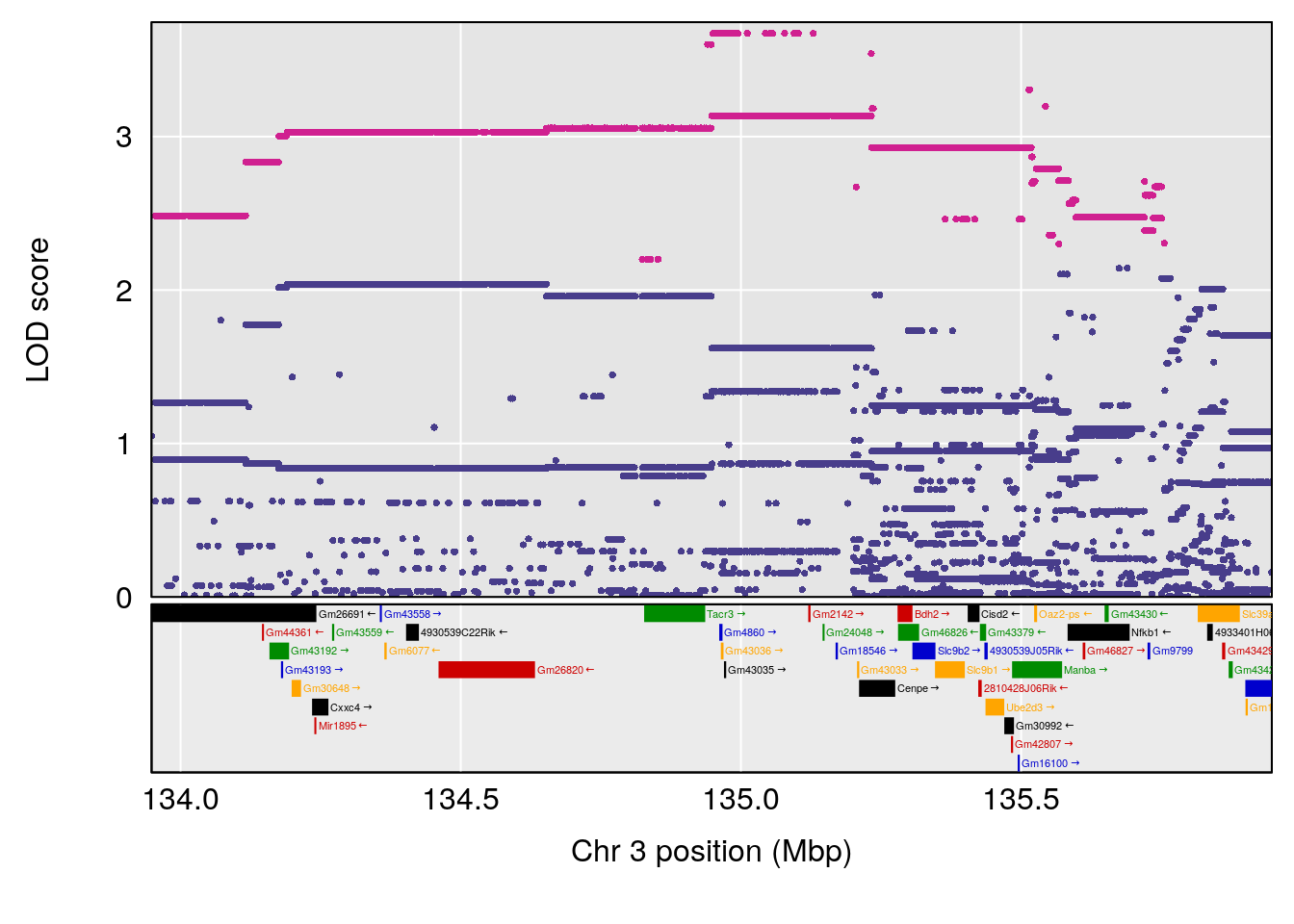
# 2 1 pheno1 3 134.90752 6.398901 129.55133 138.97690
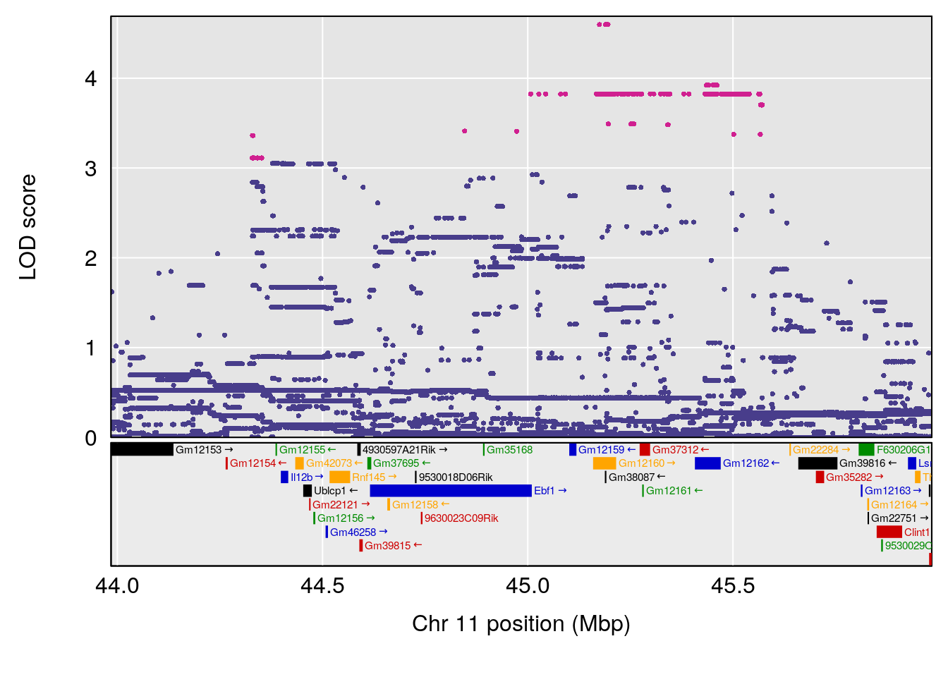
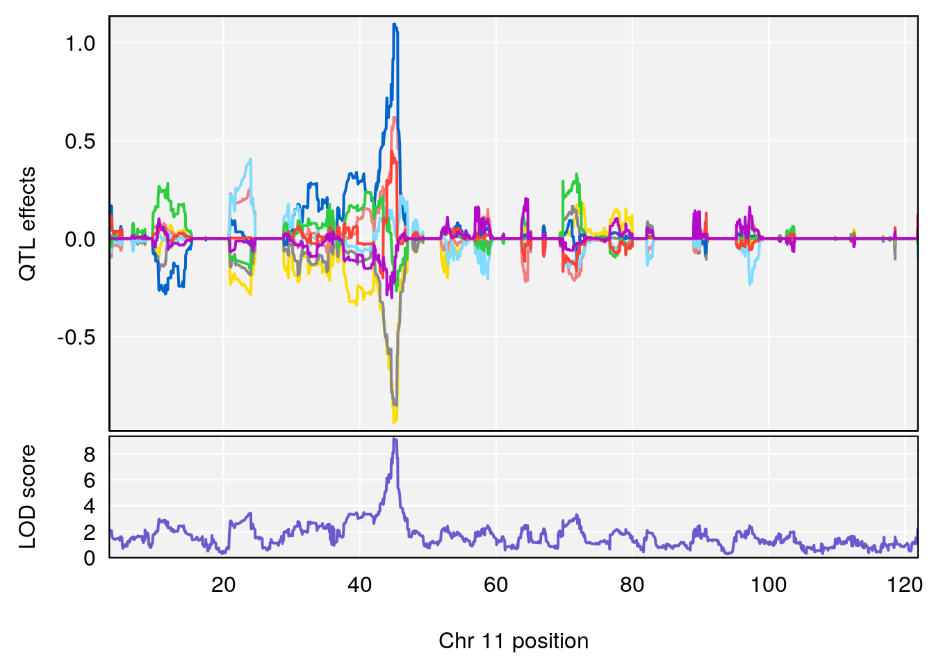
# 3 1 pheno1 11 44.98459 9.328283 44.63764 45.57241
# [1] 1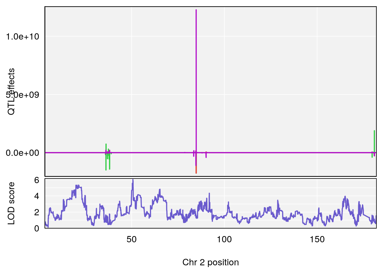
# [1] 2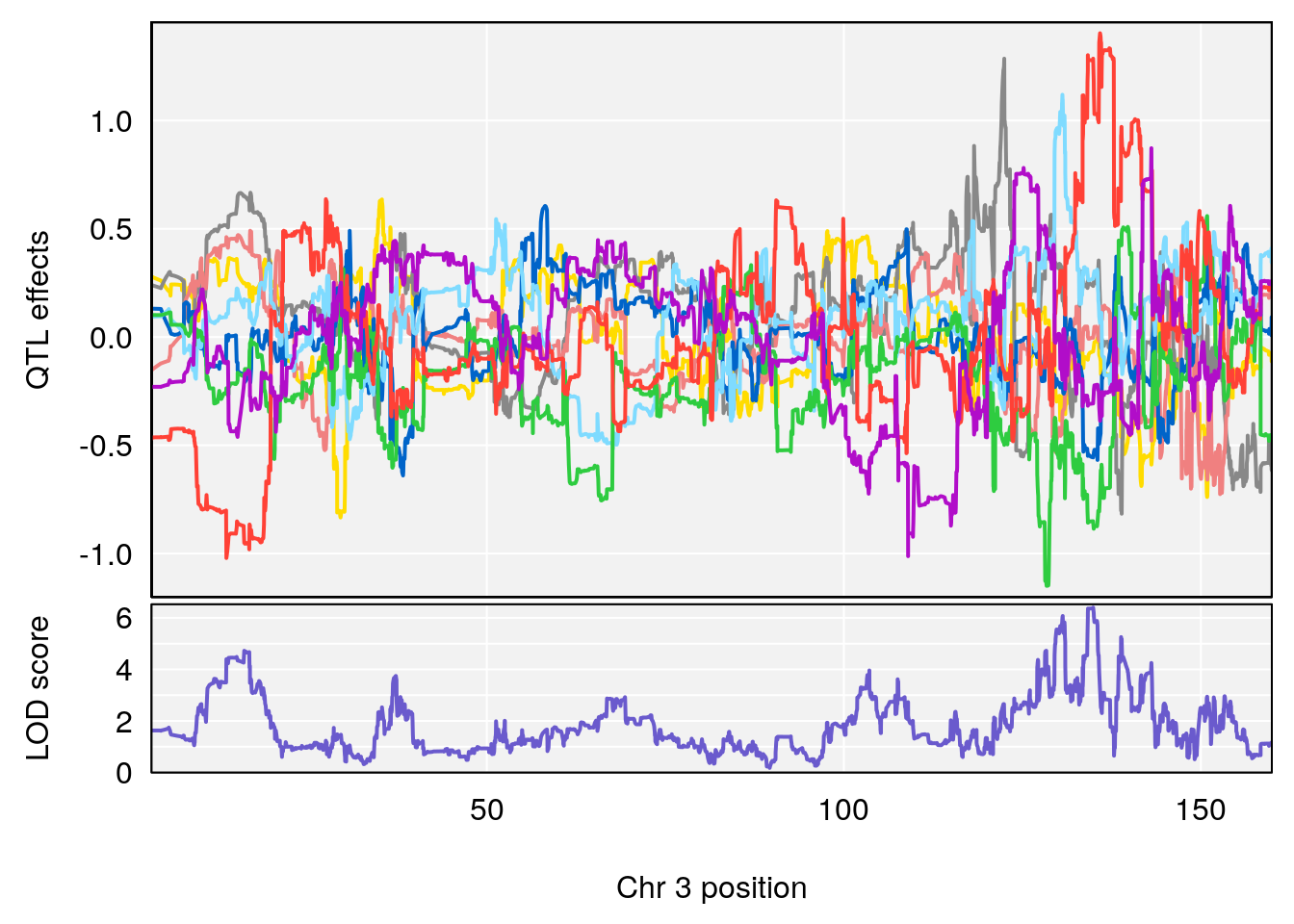
# [1] 3
# [1] "Rpef"
#   lodindex lodcolumn chr       pos      lod     ci_lo    ci_hi
# 1        1    pheno1  15  4.729387 6.279750  3.288506 92.65179
# 2        1    pheno1   X 49.136359 7.600827 47.504265 51.99289
# [1] 1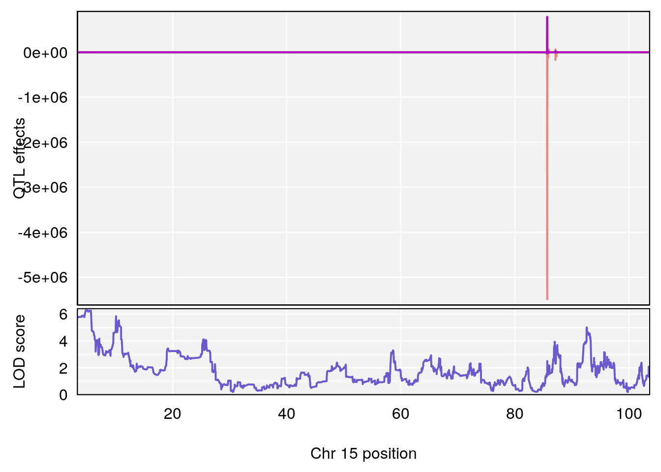
# [1] 2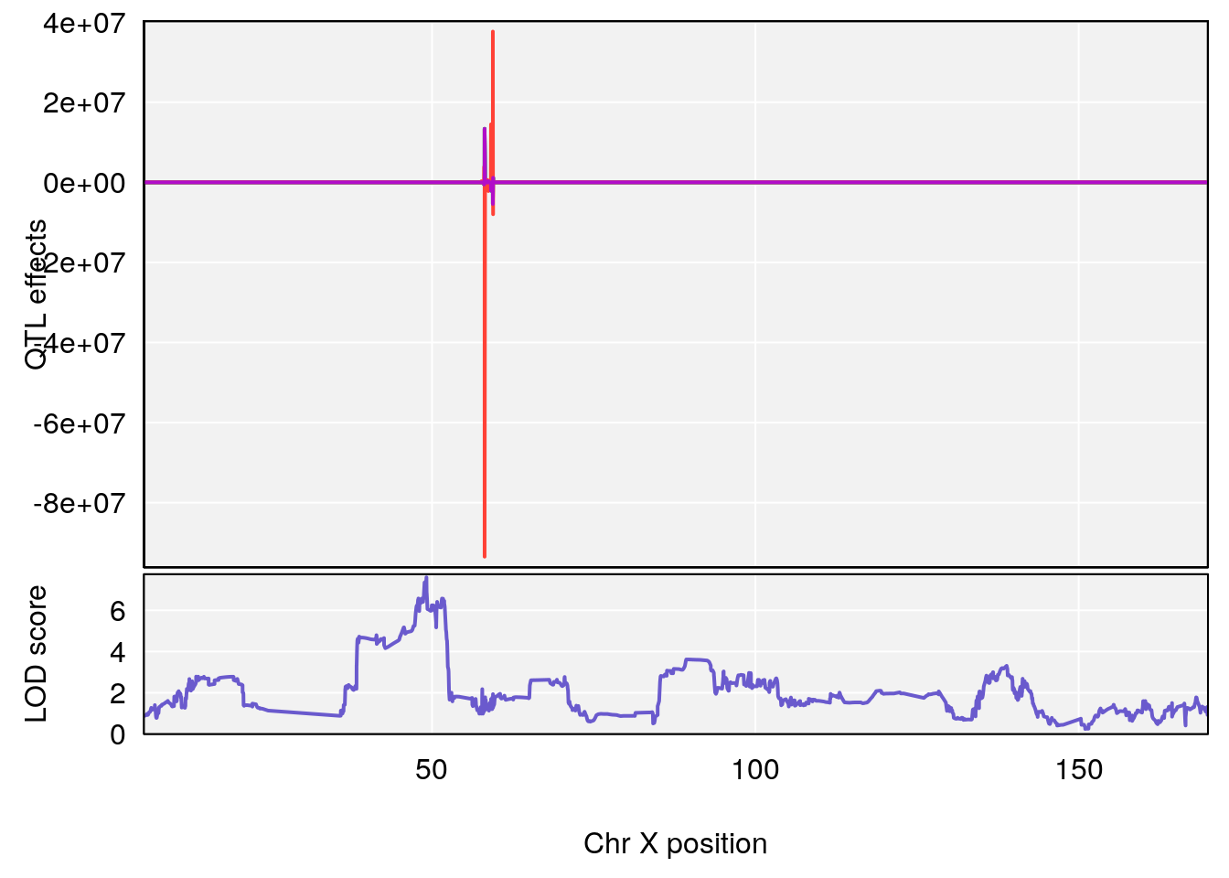
# [1] "PIFb"
#   lodindex lodcolumn chr      pos      lod    ci_lo    ci_hi
# 1        1    pheno1  18 48.14642 6.063384 28.95925 58.39852
# [1] 1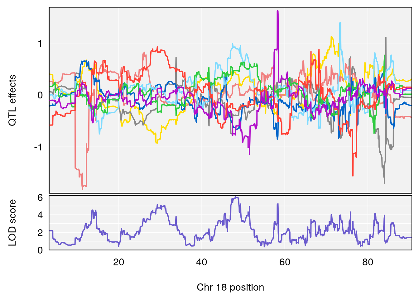
# [1] "PEFb"
#   lodindex lodcolumn chr      pos      lod    ci_lo    ci_hi
# 1        1    pheno1  17 55.28827 6.060439 4.732605 56.16387
# [1] 1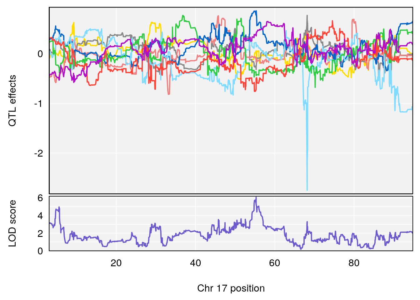
# [1] "Ti__sec"
# lodindex lodcolumn chr pos lod ci_lo ci_hi
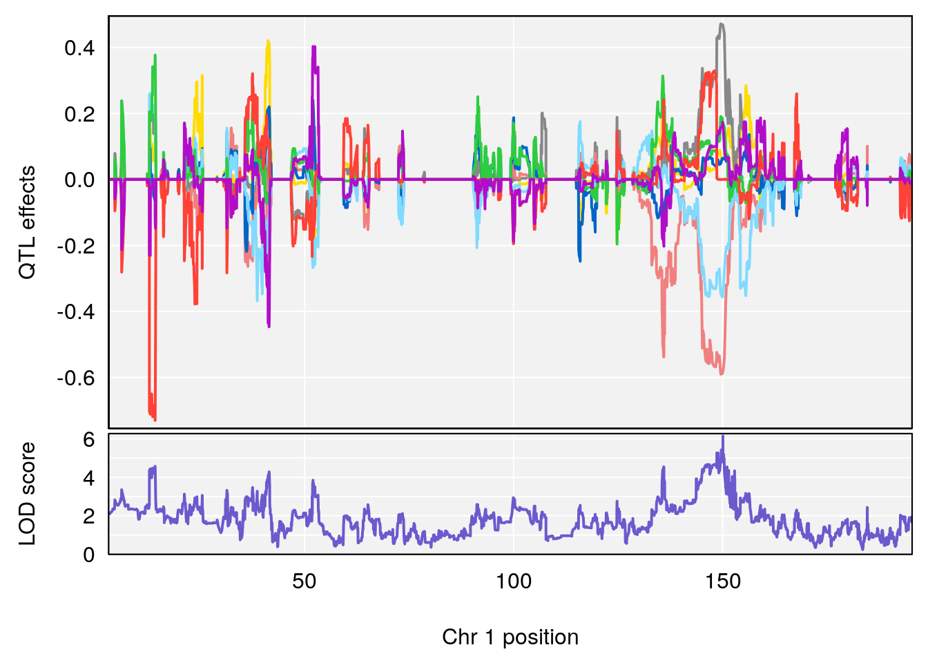
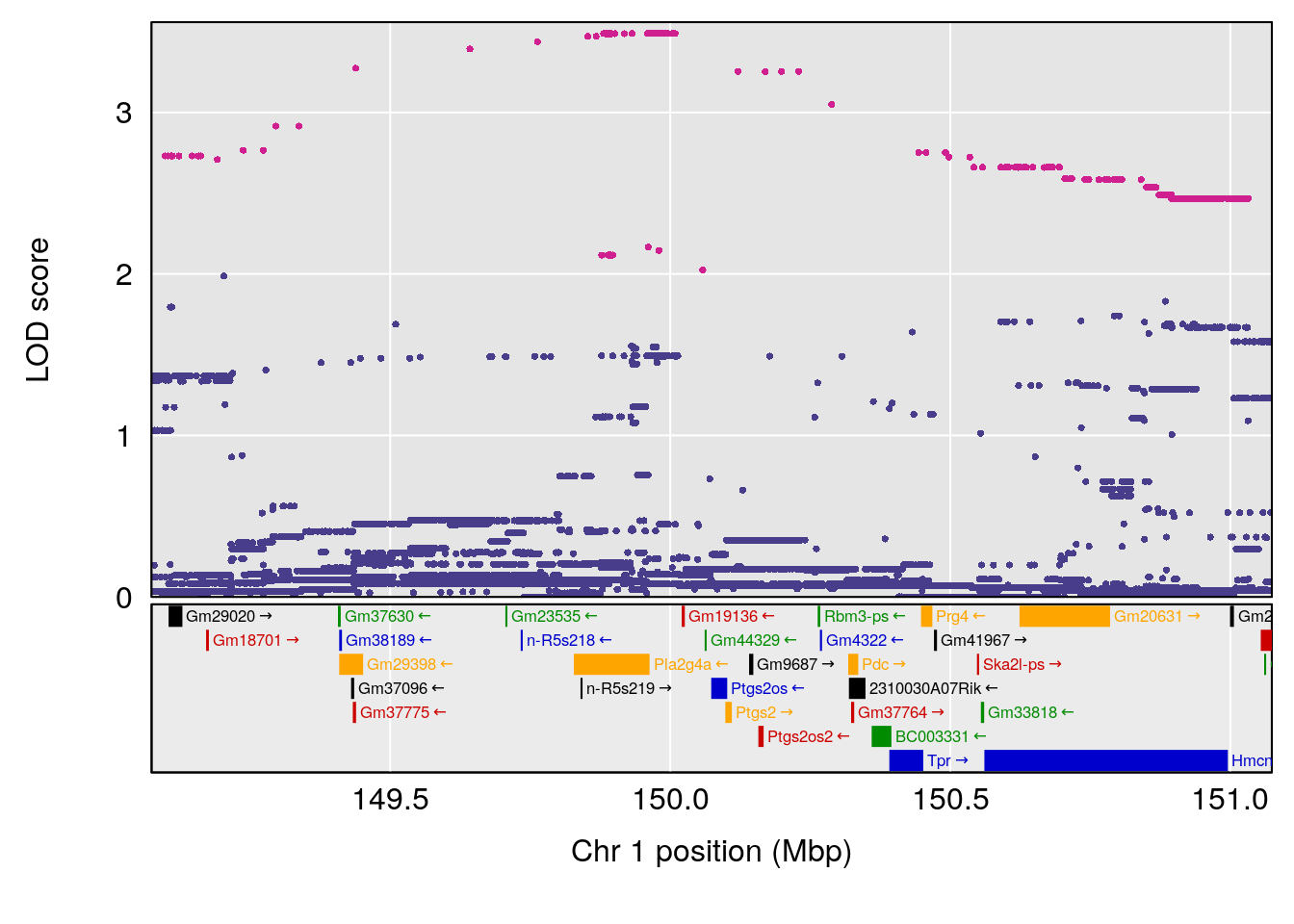
# 1 1 pheno1 1 150.07398 6.039157 139.63626 151.07520
# 2 1 pheno1 X 48.44926 6.192893 41.96483 51.89152
# [1] 1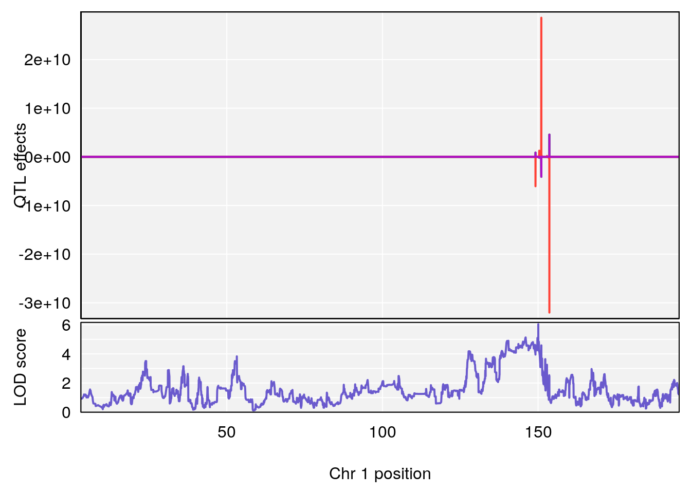
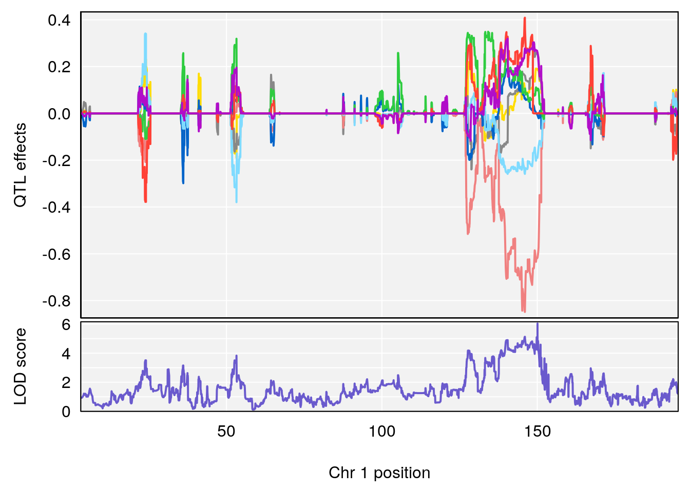
# [1] 2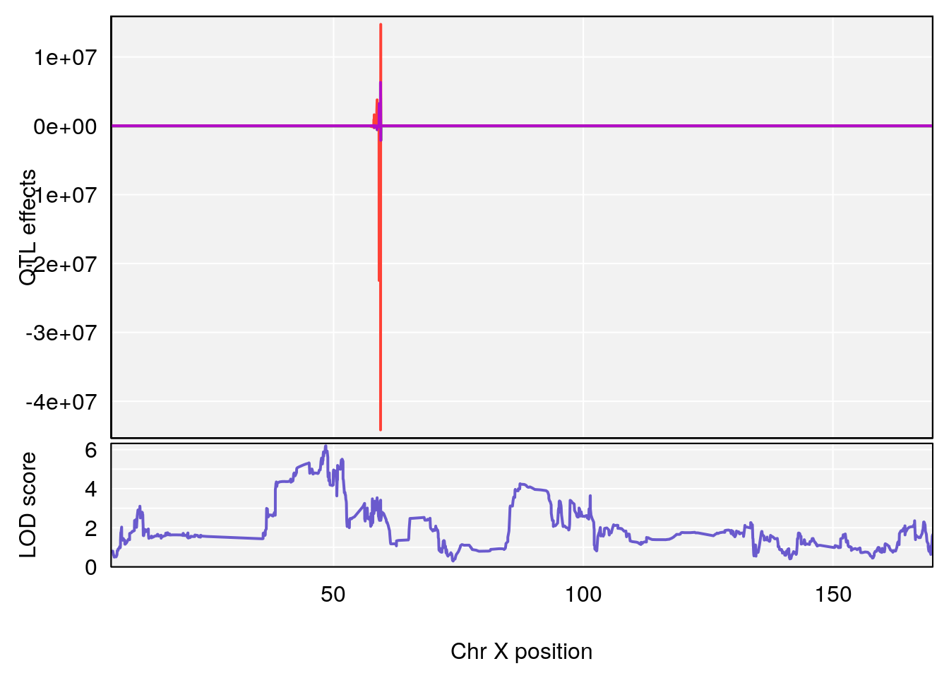
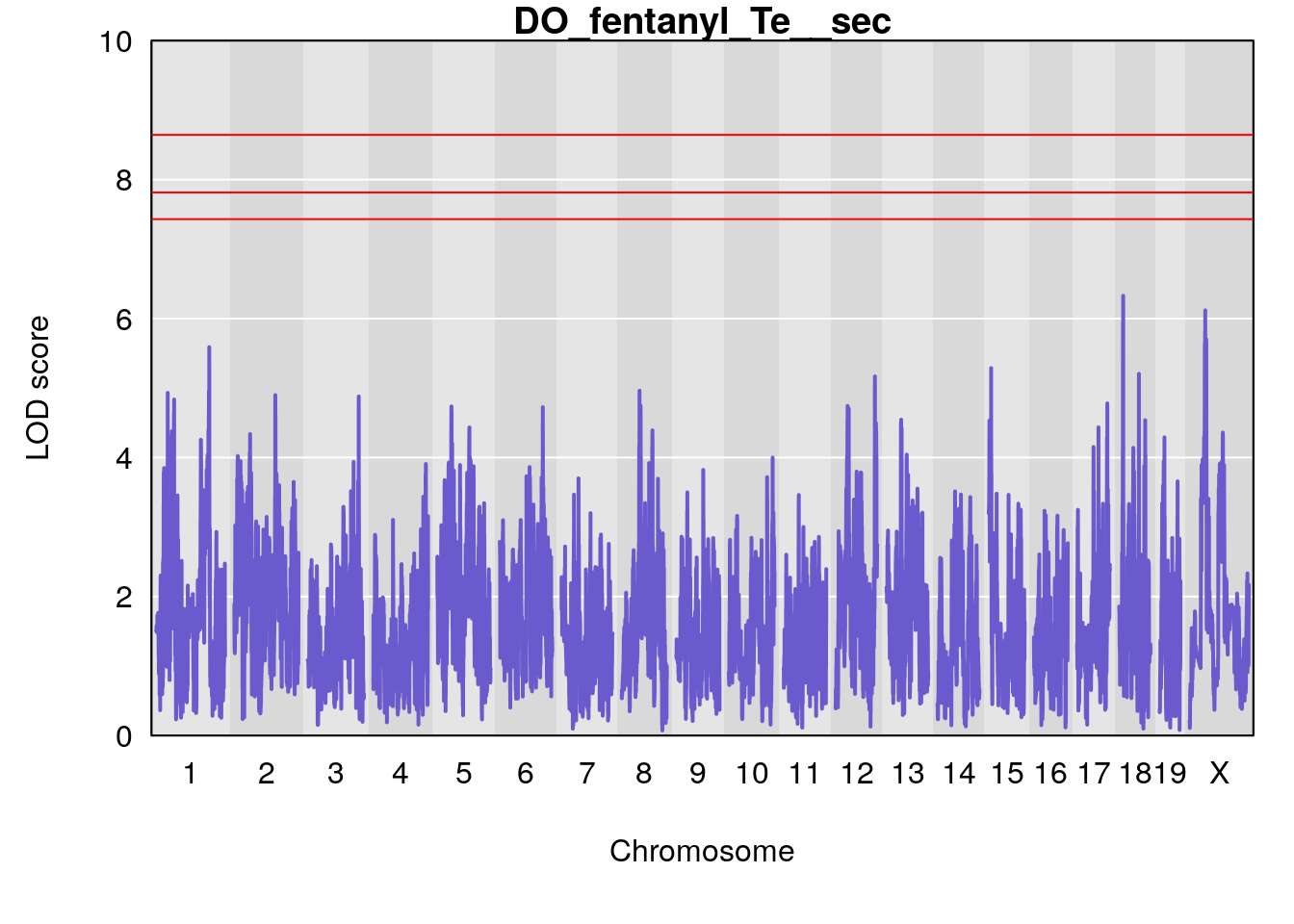
# [1] "Te__sec"
#   lodindex lodcolumn chr      pos      lod    ci_lo    ci_hi
# 1        1    pheno1  18 14.44238 6.329165 13.72254 58.36525
# 2        1    pheno1   X 48.84159 6.119243 47.31816 52.03540
# [1] 1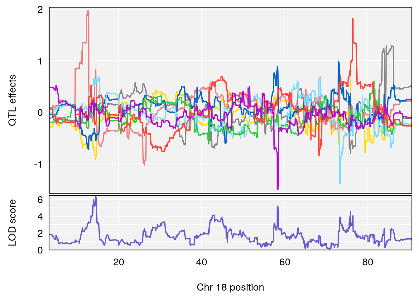
# [1] 2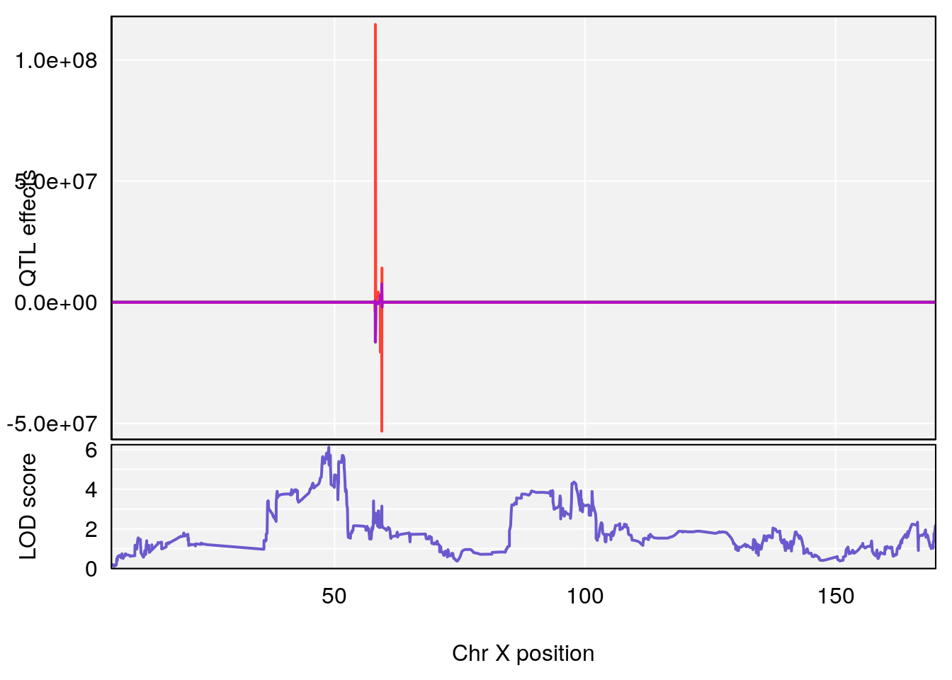
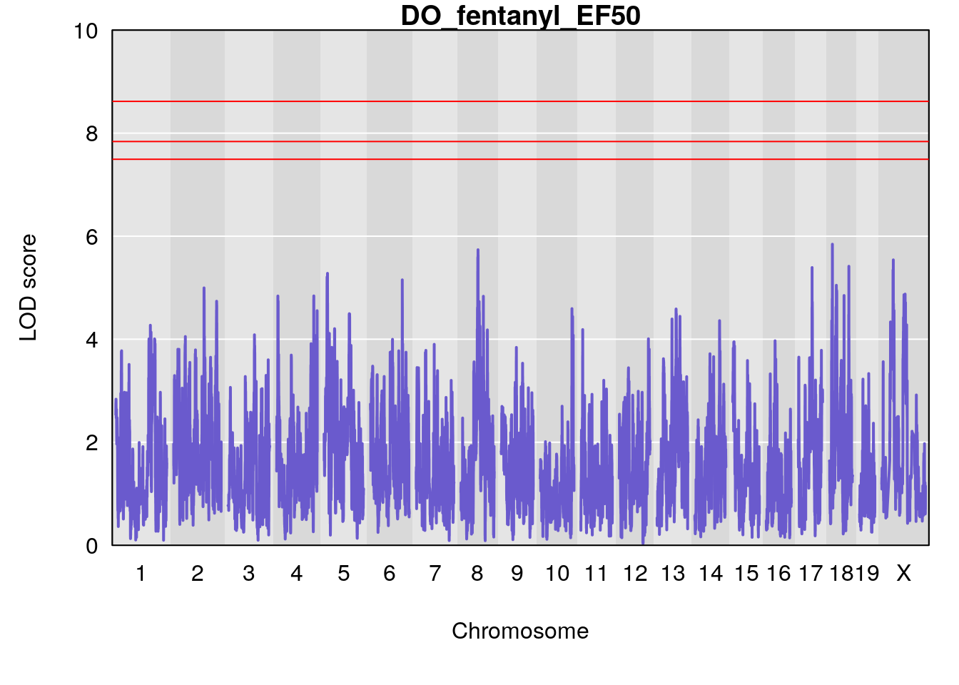
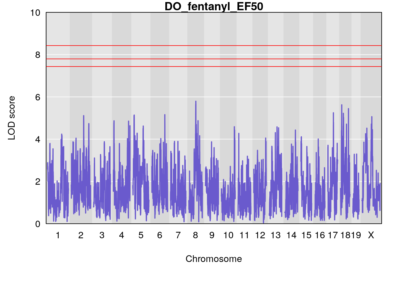
# [1] "EF50"
# [1] lodindex lodcolumn chr pos lod ci_lo ci_hi
# <0 rows> (or 0-length row.names)
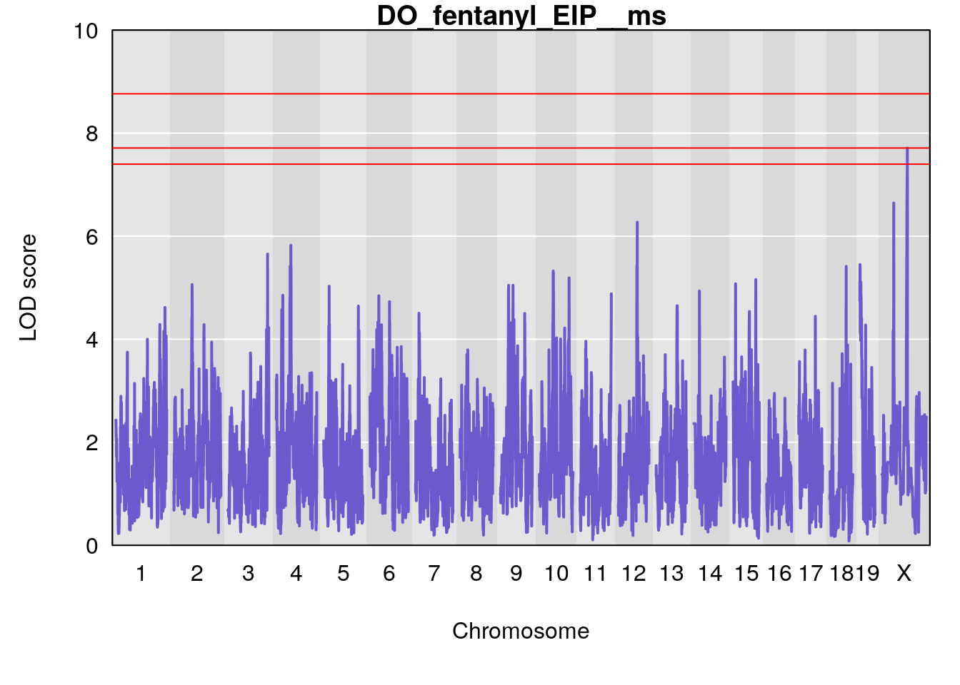
# [1] "EIP__ms"
# lodindex lodcolumn chr pos lod ci_lo ci_hi
# 1 1 pheno1 9 33.73128 6.302979 33.55617 51.33504
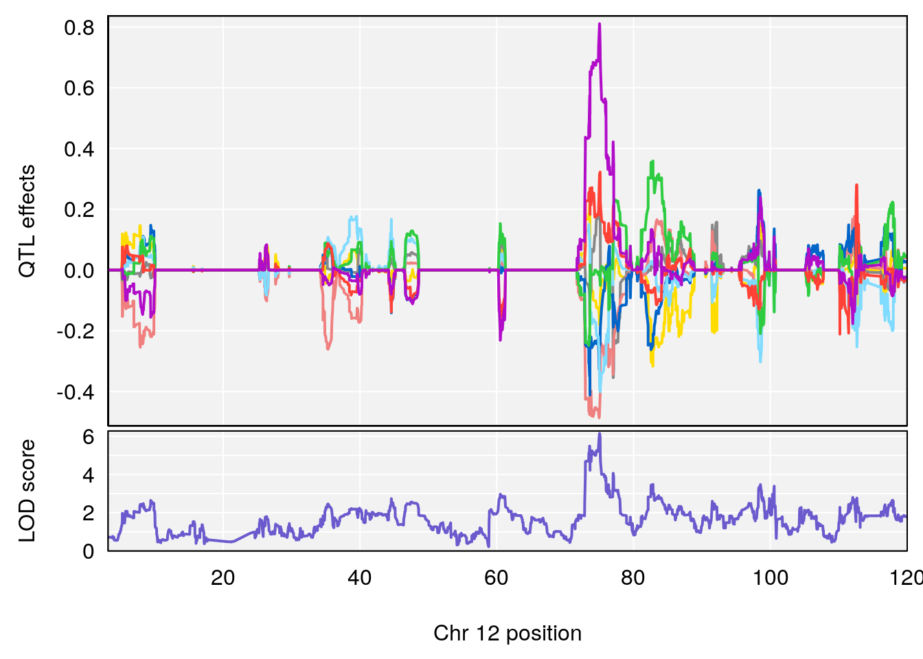
# 2 1 pheno1 12 75.02857 6.152282 72.95626 75.32827
# [1] 1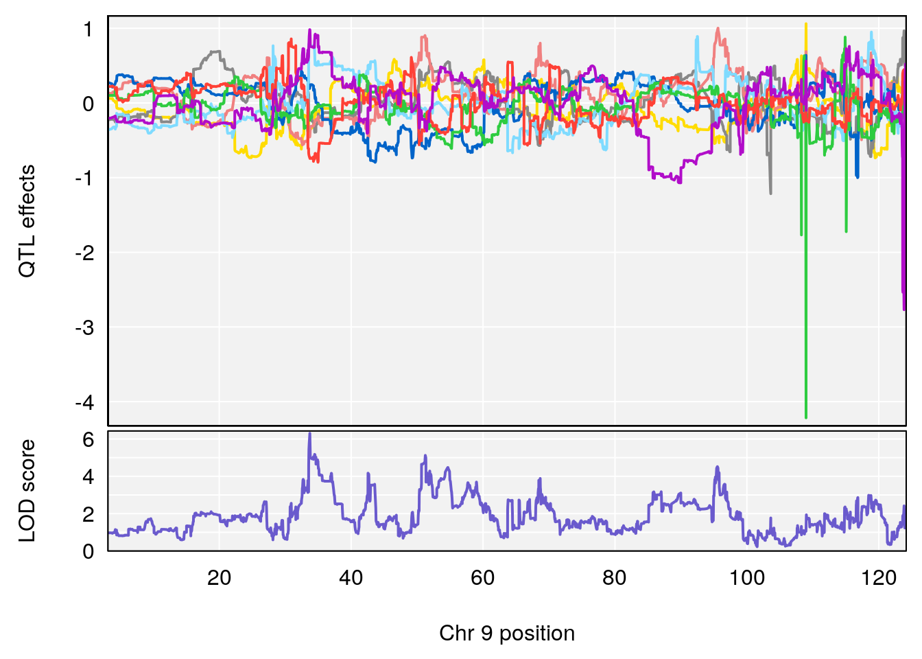
# [1] 2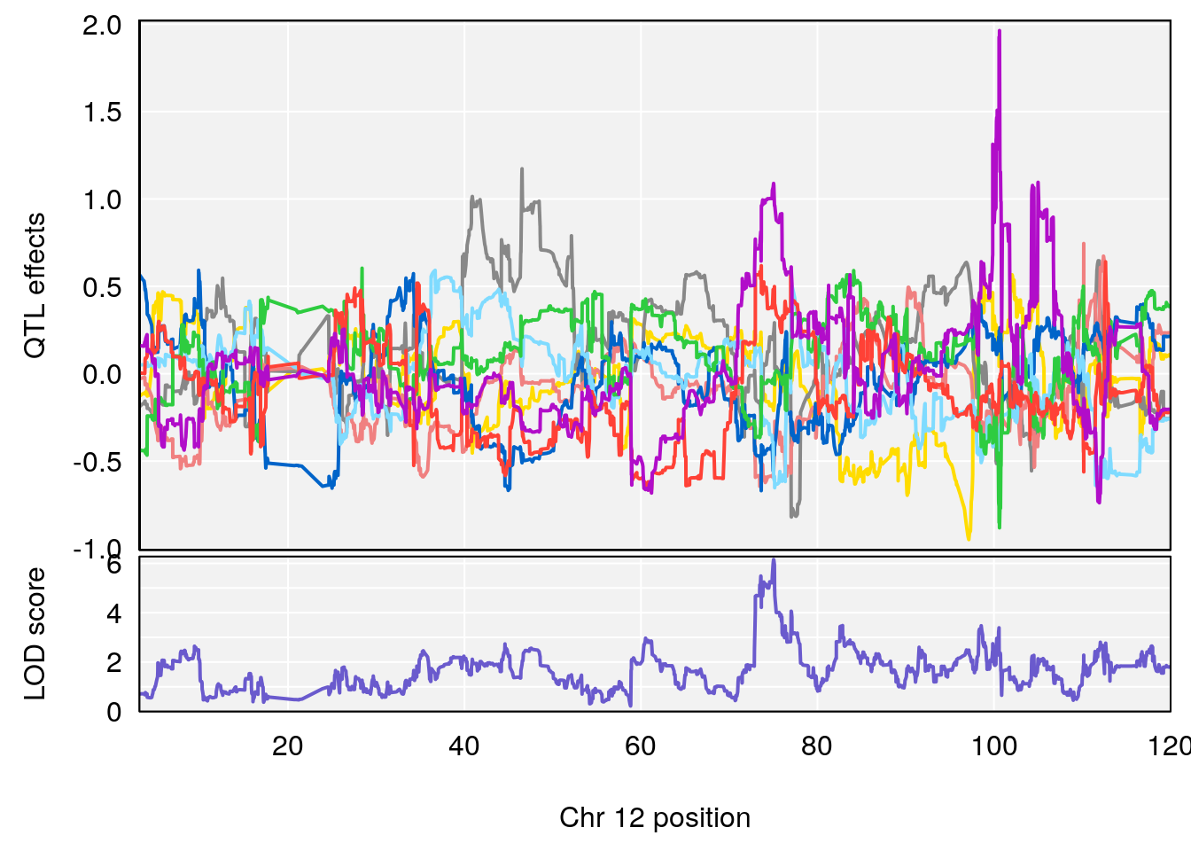
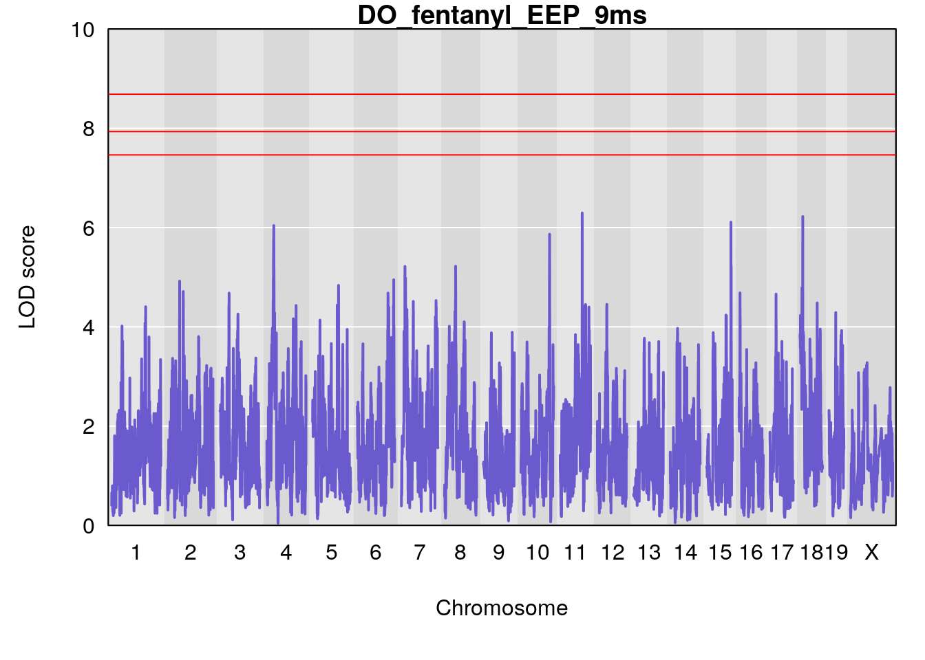
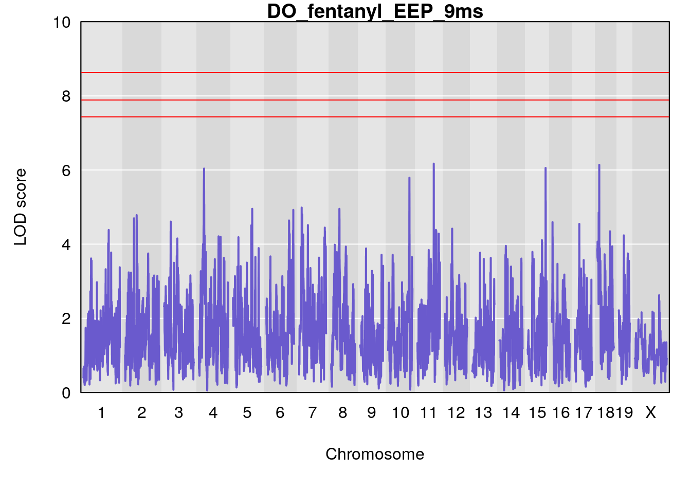
# [1] "EEP_9ms"
#   lodindex lodcolumn chr      pos      lod    ci_lo    ci_hi
# 1        1    pheno1   4 30.68259 6.041030 28.41930 31.68917
# 2        1    pheno1  11 88.96223 6.294164 88.81049 89.28146
# 3        1    pheno1  15 97.60229 6.108644 97.40501 98.51594
# 4        1    pheno1  18 13.94190 6.221707 10.84216 14.11994
# [1] 1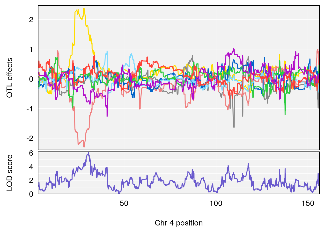
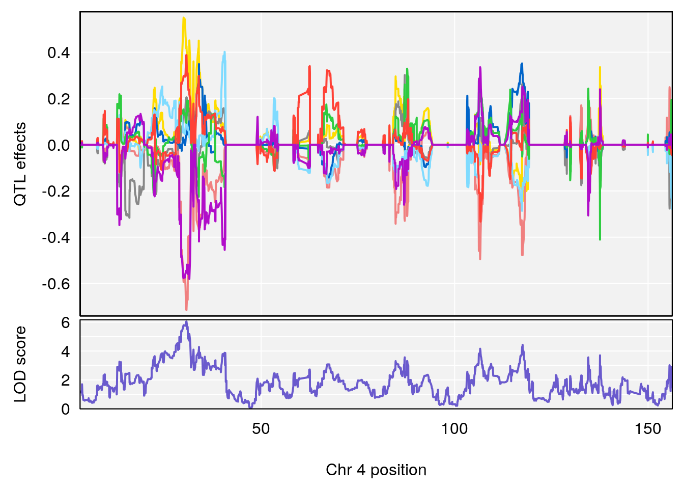

# [1] 2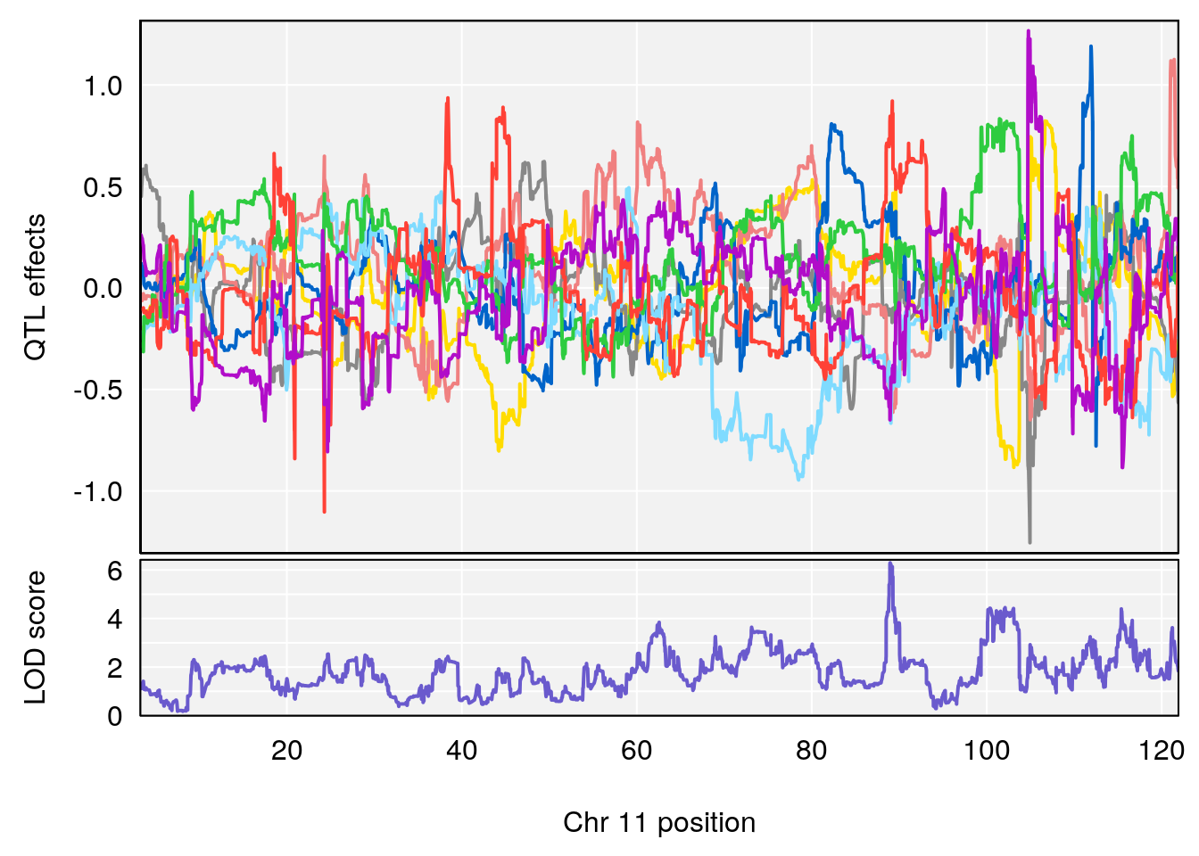
# [1] 3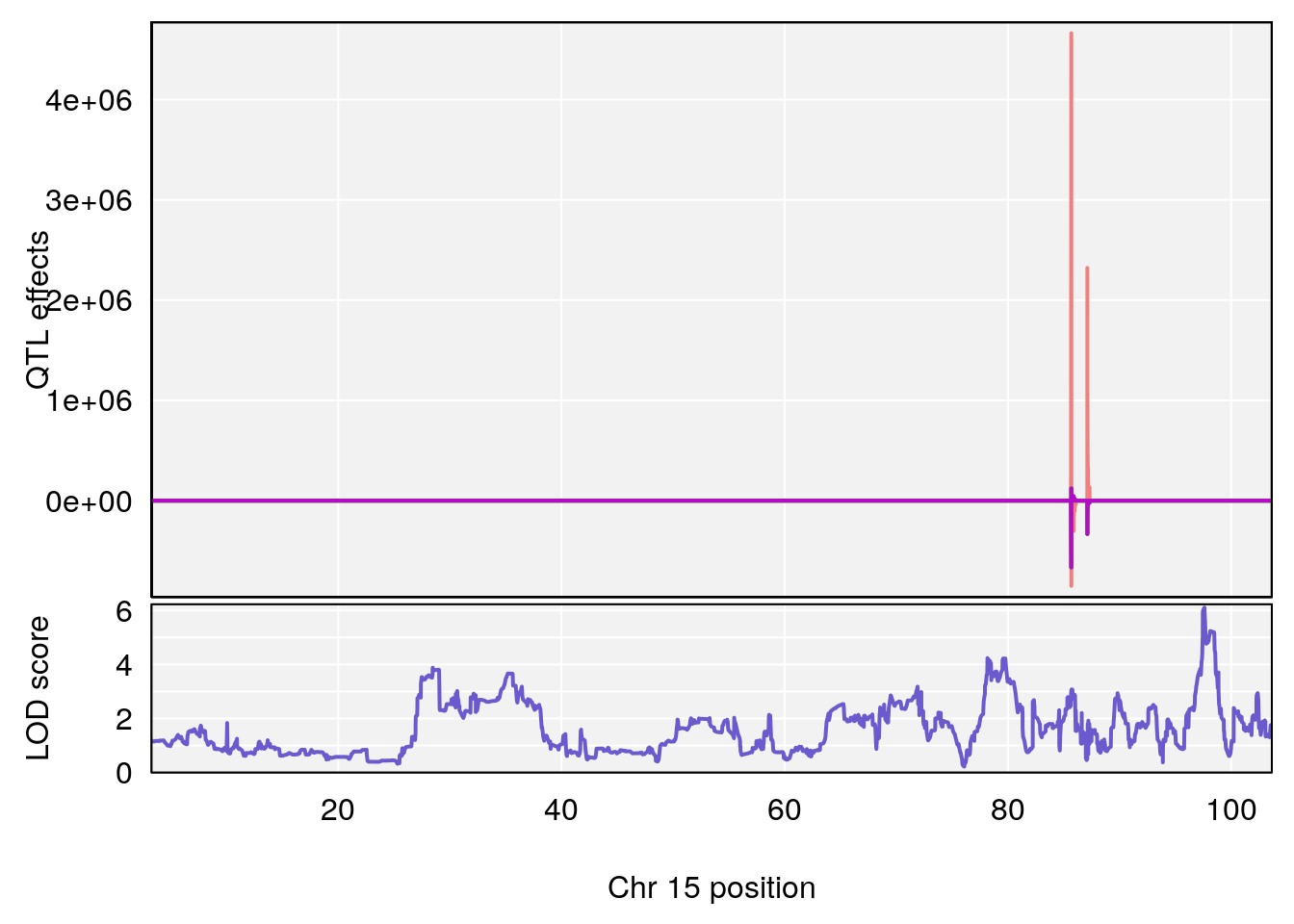
# [1] 4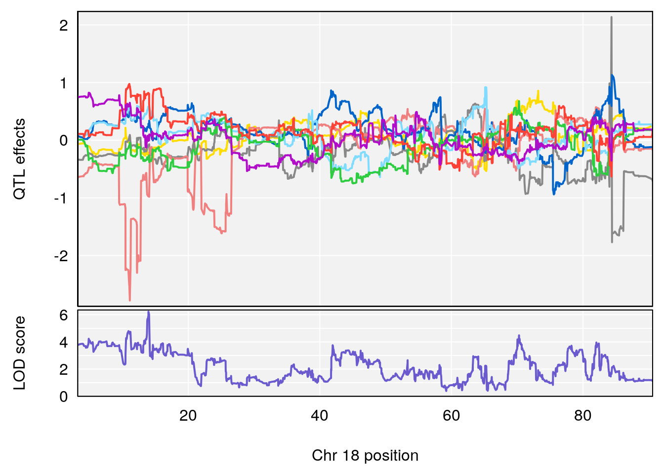
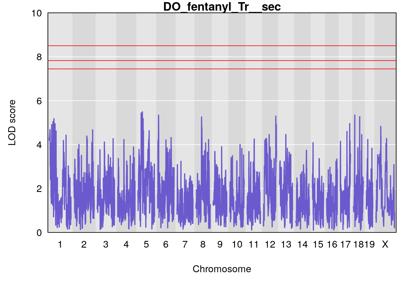
# [1] "Tr__sec"
# [1] lodindex  lodcolumn chr       pos       lod       ci_lo     ci_hi
# <0 rows> (or 0-length row.names)
# [1] "TB"
#   lodindex lodcolumn chr      pos      lod    ci_lo    ci_hi
# 1        1    pheno1  17 52.00172 6.006990 51.44475 54.75322
# 2        1    pheno1   X 47.90864 7.386139 38.62993 49.16466
# [1] 1
# [1] 2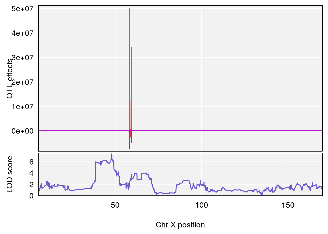
# [1] "TP"
#   lodindex lodcolumn chr       pos      lod     ci_lo     ci_hi
# 1        1    pheno1   1 150.07398 6.148673 146.26888 150.40745
# 2        1    pheno1  11  44.98459 9.179589  44.77474  45.50121
# 3        1    pheno1  12  76.37279 6.114872  75.13355  77.00267
# [1] 1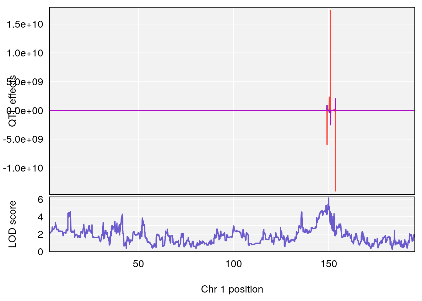
# [1] 2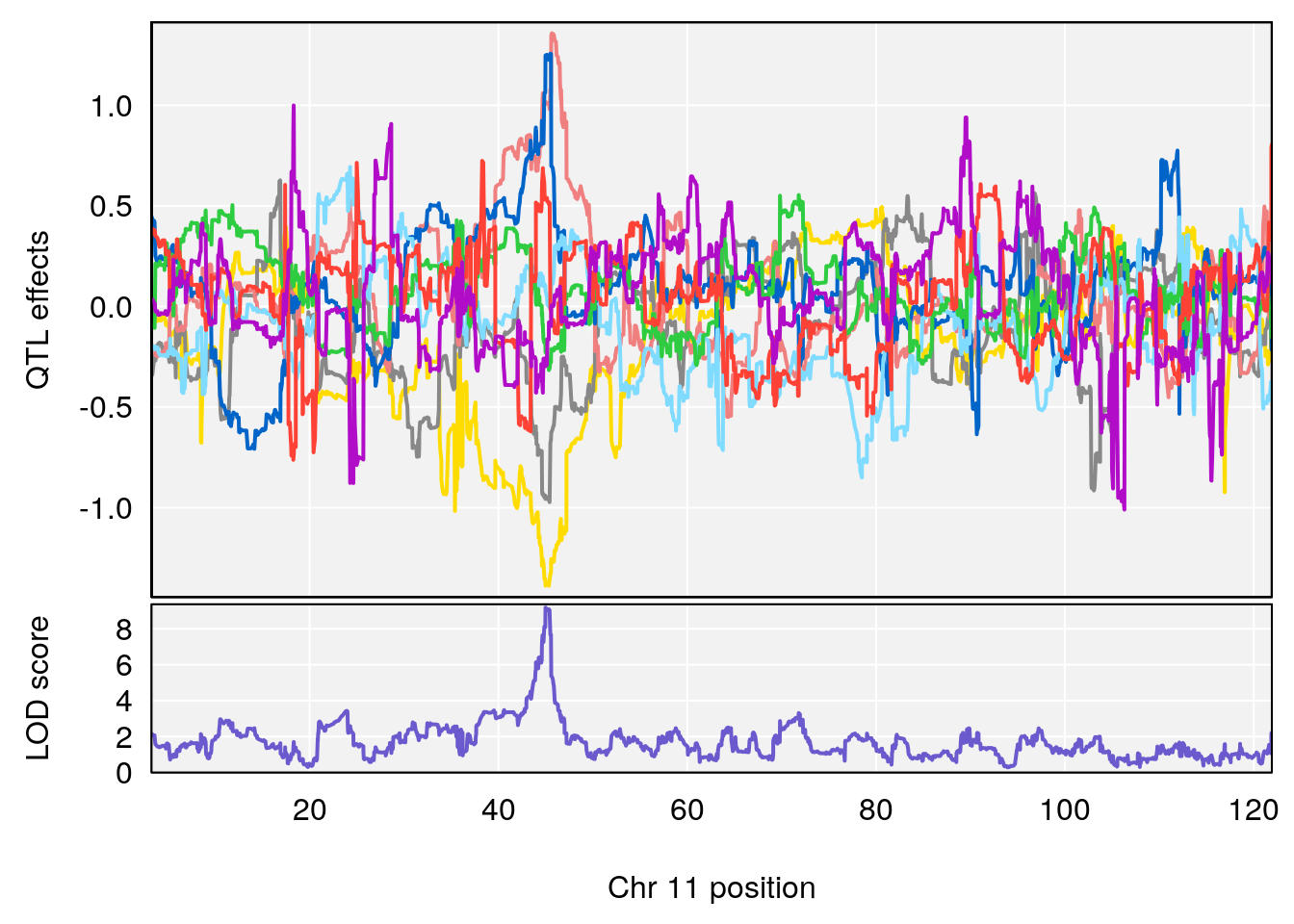
# [1] 3
# [1] "Rinx"
#   lodindex lodcolumn chr      pos      lod    ci_lo    ci_hi
# 1        1    pheno1   X 47.96484 7.570727 47.36754 49.16466
# [1] 1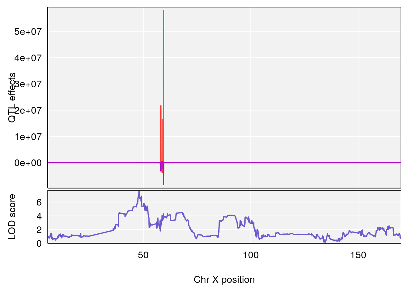
# [1] "Ttot"
#   lodindex lodcolumn chr      pos      lod    ci_lo   ci_hi
# 1        1    pheno1   X 48.84159 6.177149 47.31816 52.0354
# [1] 1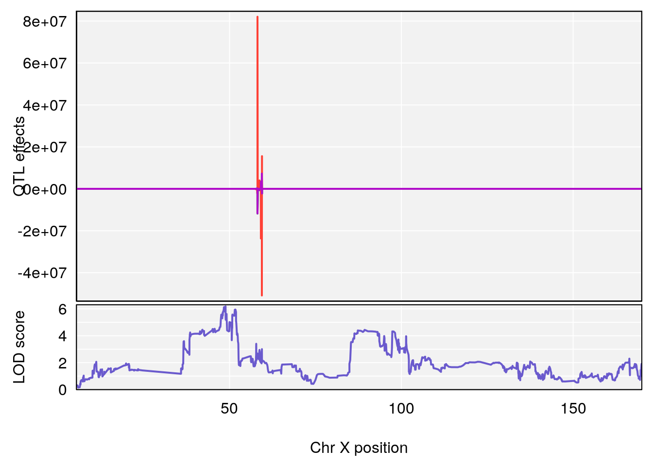
# [1] "duty_cycle"
#   lodindex lodcolumn chr      pos      lod    ci_lo     ci_hi
# 1        1    pheno1   1 14.51340 6.536959 14.29712  45.11896
# 2        1    pheno1   7 61.31511 6.261265 57.83220 138.61507
# 3        1    pheno1  12 77.04734 6.217663 76.96808  77.89729
# 4        1    pheno1  17 37.12731 6.504138 36.41471  54.21388
# [1] 1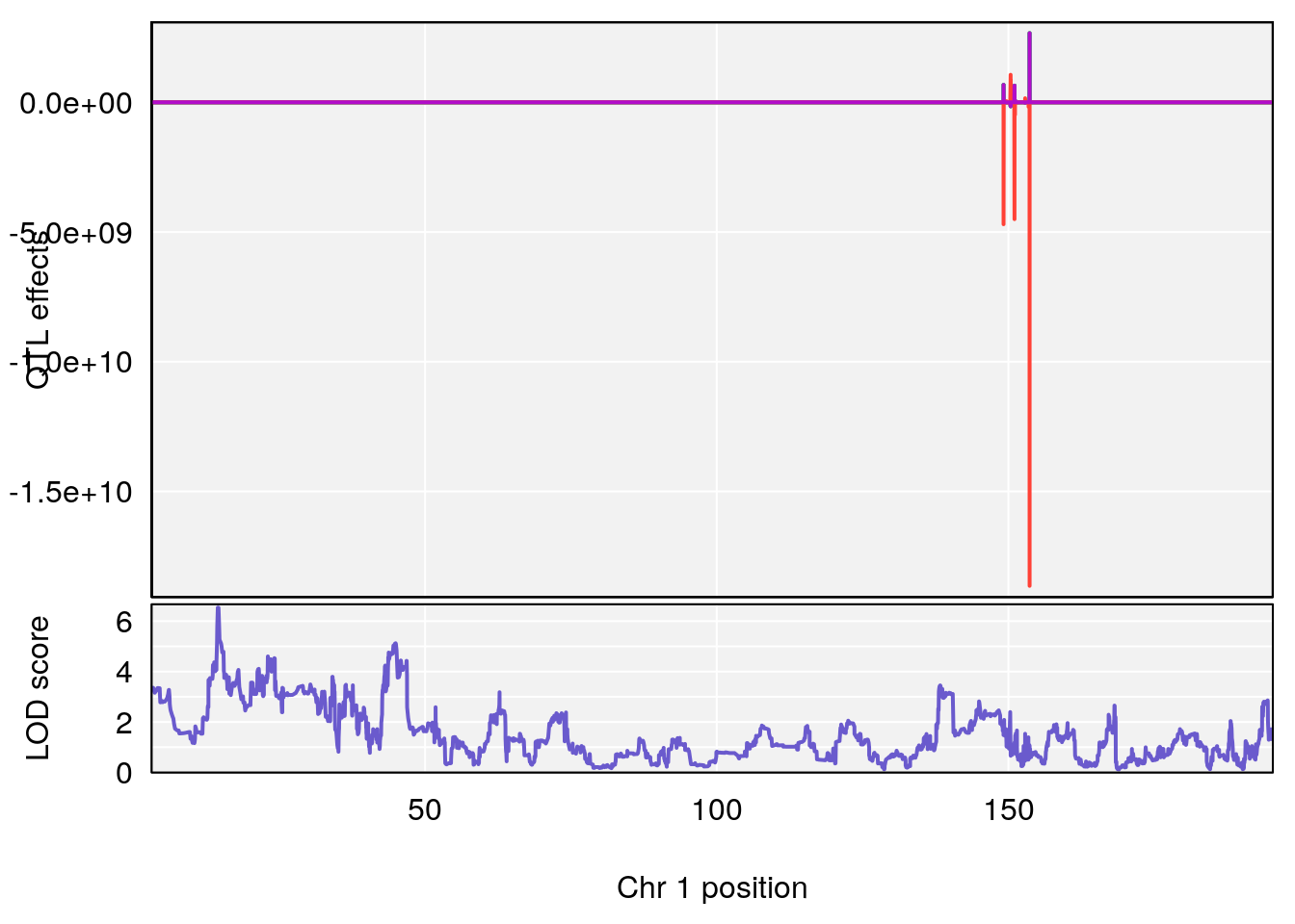
# [1] 2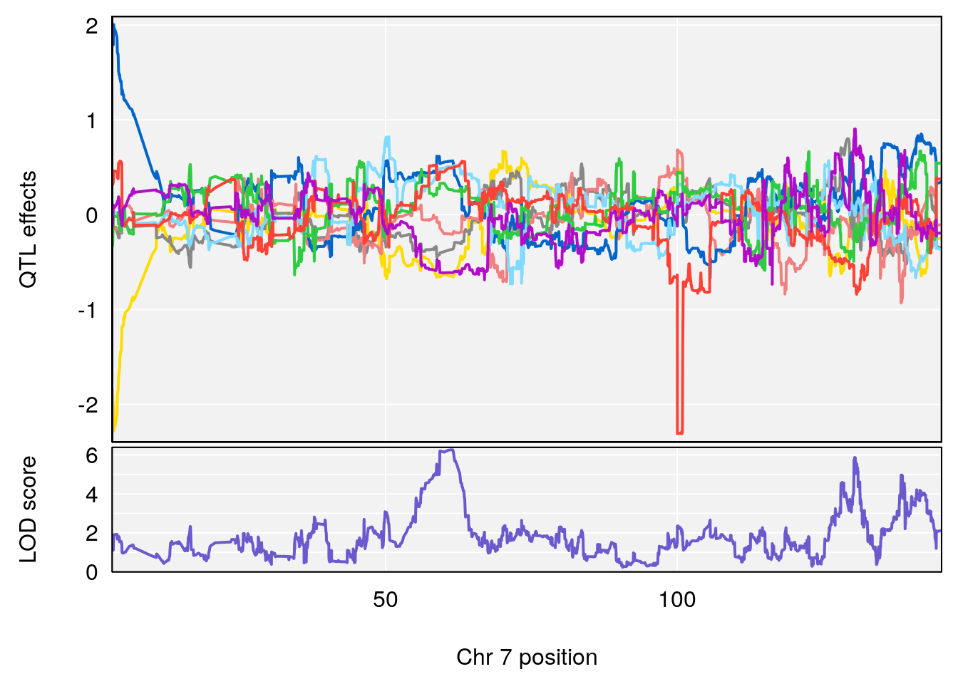
# [1] 3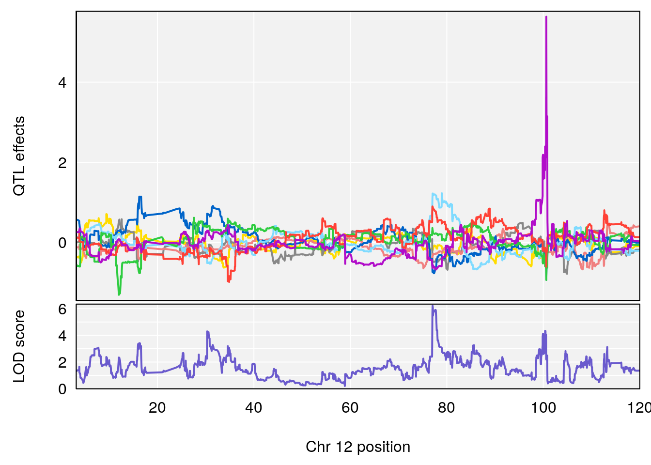
# [1] 4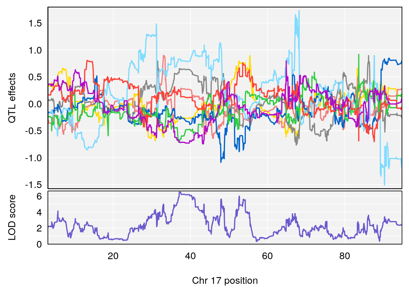

# [1] "resp_flow"
# [1] lodindex  lodcolumn chr       pos       lod       ci_lo     ci_hi
# <0 rows> (or 0-length row.names)
# [1] "insp_flow"
#   lodindex lodcolumn chr      pos      lod    ci_lo    ci_hi
# 1        1    pheno1  17 55.28827 6.308378 54.27183 55.45841
# 2        1    pheno1  18 48.14642 6.127945 29.23075 51.53735
# [1] 1
# [1] 2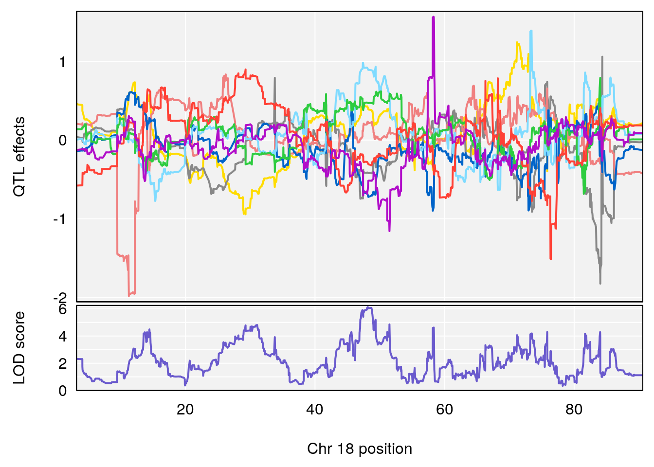
# [1] "exp_flow"
# [1] lodindex lodcolumn chr pos lod ci_lo ci_hi
# <0 rows> (or 0-length row.names)
#save peaks coeff plot
for(i in names(qtl.morphine.out)){
print(i)
peaks <- find_peaks(qtl.morphine.out[[i]], map=gm$pmap, threshold=6, drop=1.5)
fname <- paste("output/Fentanyl/DO_fentanyl_",i,"_coefplot.pdf",sep="")
pdf(file = fname, width = 16, height =8)
if(dim(peaks)[1] != 0){
for(p in 1:dim(peaks)[1]) {
print(p)
chr <-peaks[p,3]
#coeff plot
par(mar=c(4.1, 4.1, 0.6, 0.6))
plot_coefCC(coef_c1[[i]][[p]], gm$pmap[chr], scan1_output=qtl.morphine.out[[i]], bgcolor="gray95", legend=NULL)
plot_coefCC(coef_c2[[i]][[p]], gm$pmap[chr], scan1_output=qtl.morphine.out[[i]], bgcolor="gray95", legend=NULL)
plot(out_snps[[i]][[p]]$lod, out_snps[[i]][[p]]$snpinfo, drop_hilit=1.5, genes=out_genes[[i]][[p]])
}
}
dev.off()
}
# [1] "Survival.Time"
# [1] 1
# [1] "Recovery.Time"
# [1] 1
# [1] "Min.depression"
# [1] 1
# [1] "Status_bin"
# [1] 1
# [1] 2
# [1] 3
# [1] "f__Bpm"
# [1] 1
# [1] 2
# [1] "TVb_ml"
# [1] 1
# [1] 2
# [1] 3
# [1] "MVb__ml_min"
# [1] 1
# [1] "Penh"
# [1] 1
# [1] 2
# [1] "PAU"
# [1] 1
# [1] 2
# [1] 3
# [1] "Rpef"
# [1] 1
# [1] 2
# [1] "PIFb"
# [1] 1
# [1] "PEFb"
# [1] 1
# [1] "Ti__sec"
# [1] 1
# [1] 2
# [1] "Te__sec"
# [1] 1
# [1] 2
# [1] "EF50"
# [1] "EIP__ms"
# [1] 1
# [1] 2
# [1] "EEP_9ms"
# [1] 1
# [1] 2
# [1] 3
# [1] 4
# [1] "Tr__sec"
# [1] "TB"
# [1] 1
# [1] 2
# [1] "TP"
# [1] 1
# [1] 2
# [1] 3
# [1] "Rinx"
# [1] 1
# [1] "Ttot"
# [1] 1
# [1] "duty_cycle"
# [1] 1
# [1] 2
# [1] 3
# [1] 4
# [1] "resp_flow"
# [1] "insp_flow"
# [1] 1
# [1] 2
# [1] "exp_flow"
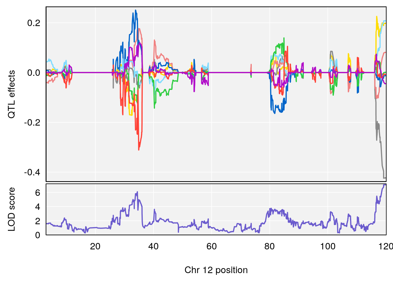
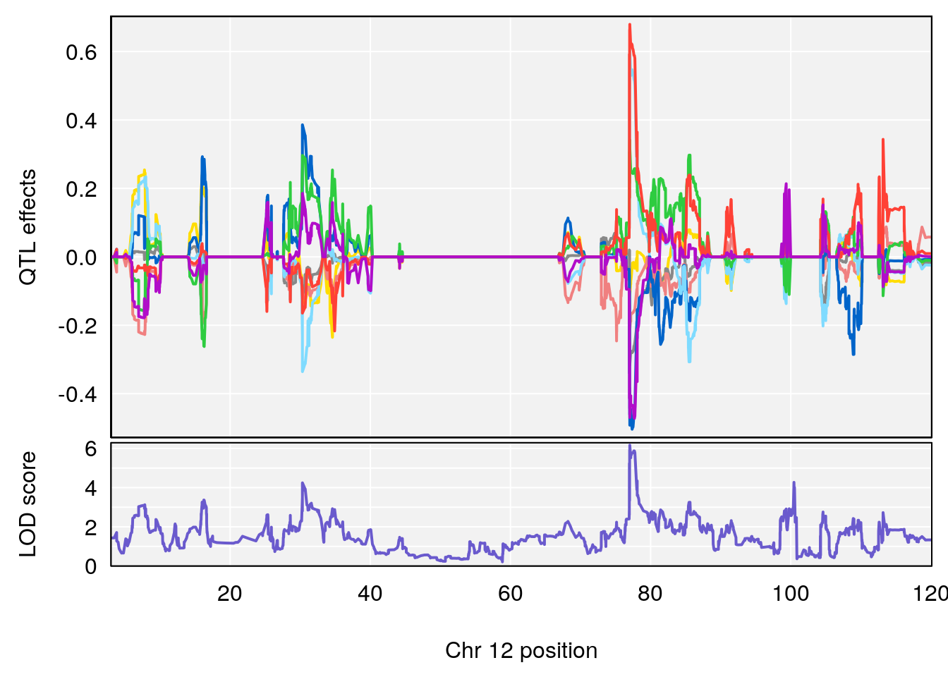
#save peaks coeff blup plot
for(i in names(qtl.morphine.out)){
print(i)
peaks <- find_peaks(qtl.morphine.out[[i]], map=gm$pmap, threshold=6, drop=1.5)
fname <- paste("output/Fentanyl/DO_fentanyl_",i,"_coefplot_blup.pdf",sep="")
pdf(file = fname, width = 16, height =8)
if(dim(peaks)[1] != 0){
for(p in 1:dim(peaks)[1]) {
print(p)
chr <-peaks[p,3]
#coeff plot
par(mar=c(4.1, 4.1, 0.6, 0.6))
plot_coefCC(coef_c1[[i]][[p]], gm$pmap[chr], scan1_output=qtl.morphine.out[[i]], bgcolor="gray95", legend=NULL)
plot_coefCC(coef_c2[[i]][[p]], gm$pmap[chr], scan1_output=qtl.morphine.out[[i]], bgcolor="gray95", legend=NULL)
plot(out_snps[[i]][[p]]$lod, out_snps[[i]][[p]]$snpinfo, drop_hilit=1.5, genes=out_genes[[i]][[p]])
}
}
dev.off()
}
# [1] "Survival.Time"
# [1] 1
# [1] "Recovery.Time"
# [1] 1
# [1] "Min.depression"
# [1] 1
# [1] "Status_bin"
# [1] 1
# [1] 2
# [1] 3
# [1] "f__Bpm"
# [1] 1
# [1] 2
# [1] "TVb_ml"
# [1] 1
# [1] 2
# [1] 3
# [1] "MVb__ml_min"
# [1] 1
# [1] "Penh"
# [1] 1
# [1] 2
# [1] "PAU"
# [1] 1
# [1] 2
# [1] 3
# [1] "Rpef"
# [1] 1
# [1] 2
# [1] "PIFb"
# [1] 1
# [1] "PEFb"
# [1] 1
# [1] "Ti__sec"
# [1] 1
# [1] 2
# [1] "Te__sec"
# [1] 1
# [1] 2
# [1] "EF50"
# [1] "EIP__ms"
# [1] 1
# [1] 2
# [1] "EEP_9ms"
# [1] 1
# [1] 2
# [1] 3
# [1] 4
# [1] "Tr__sec"
# [1] "TB"
# [1] 1
# [1] 2
# [1] "TP"
# [1] 1
# [1] 2
# [1] 3
# [1] "Rinx"
# [1] 1
# [1] "Ttot"
# [1] 1
# [1] "duty_cycle"
# [1] 1
# [1] 2
# [1] 3
# [1] 4
# [1] "resp_flow"
# [1] "insp_flow"
# [1] 1
# [1] 2
# [1] "exp_flow"Plot qtl mapping on 69K
load("output/Fentanyl/qtl.fentanyl.69k.out.RData")
#pmap and gmap
load("data/69k_grid_pgmap.RData")

#genome-wide plot
for(i in names(qtl.morphine.out)){
  par(mar=c(5.1, 4.1, 1.1, 1.1))
  ymx <- maxlod(qtl.morphine.out[[i]]) # overall maximum LOD score
  plot(qtl.morphine.out[[i]], map=pmap, lodcolumn=1, col="slateblue", ylim=c(0, 10))
  abline(h=summary(qtl.morphine.operm[[i]], alpha=c(0.10, 0.05, 0.01))[[1]], col="red")
  abline(h=summary(qtl.morphine.operm[[i]], alpha=c(0.10, 0.05, 0.01))[[2]], col="red")
  abline(h=summary(qtl.morphine.operm[[i]], alpha=c(0.10, 0.05, 0.01))[[3]], col="red")
  title(main = paste0("DO_fentanyl_",i))
}
| Version | Author | Date |
|---|---|---|
| 3f2fa84 | xhyuo | 2021-09-06 |


#save genome-wide plot
for(i in names(qtl.morphine.out)){
  png(file = paste0("output/Fentanyl/DO_fentanyl_69k_", i, ".png"), width = 16, height =8, res=300, units = "in")
  par(mar=c(5.1, 4.1, 1.1, 1.1))
  ymx <- maxlod(qtl.morphine.out[[i]]) # overall maximum LOD score
  plot(qtl.morphine.out[[i]], map=pmap, lodcolumn=1, col="slateblue", ylim=c(0, 10))
  abline(h=summary(qtl.morphine.operm[[i]], alpha=c(0.10, 0.05, 0.01))[[1]], col="red")
  abline(h=summary(qtl.morphine.operm[[i]], alpha=c(0.10, 0.05, 0.01))[[2]], col="red")
  abline(h=summary(qtl.morphine.operm[[i]], alpha=c(0.10, 0.05, 0.01))[[3]], col="red")
  title(main = paste0("DO_fentanyl_",i))
  dev.off()
}

#peaks coeff plot
for(i in names(qtl.morphine.out)){
  print(i)
  peaks <- find_peaks(qtl.morphine.out[[i]], map=pmap, threshold=6, drop=1.5)
  print(peaks)
  if(dim(peaks)[1] != 0){
    for(p in 1:dim(peaks)[1]) {
    print(p)
    chr <-peaks[p,3]
    #coeff plot
    par(mar=c(4.1, 4.1, 0.6, 0.6))
    plot_coefCC(coef_c1[[i]][[p]], pmap[chr], scan1_output=qtl.morphine.out[[i]], bgcolor="gray95", legend=NULL)
    plot_coefCC(coef_c2[[i]][[p]], pmap[chr], scan1_output=qtl.morphine.out[[i]], bgcolor="gray95", legend=NULL)
    plot(out_snps[[i]][[p]]$lod, out_snps[[i]][[p]]$snpinfo, drop_hilit=1.5, genes=out_genes[[i]][[p]])
  }
  }
}
# [1] "Survival.Time"
#   lodindex lodcolumn chr      pos      lod    ci_lo   ci_hi
# 1        1    pheno1  19 35.79253 6.215615 35.44422 37.4803
# [1] 1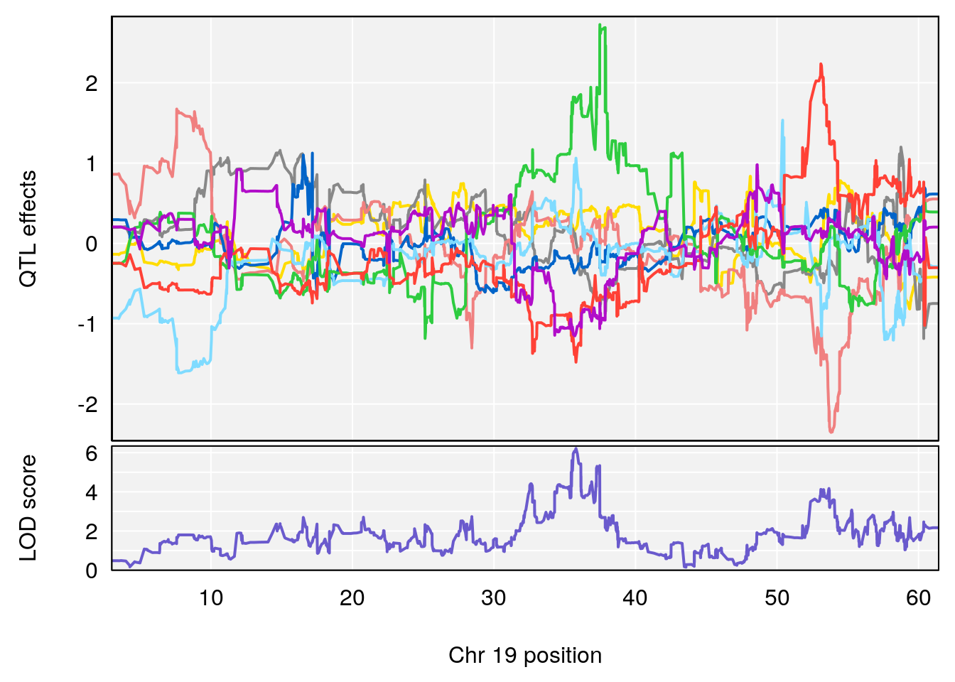
| Version | Author | Date |
|---|---|---|
| 9b57b94 | xhyuo | 2021-10-22 |
| Version | Author | Date |
|---|---|---|
| 9b57b94 | xhyuo | 2021-10-22 |
| Version | Author | Date |
|---|---|---|
| 9b57b94 | xhyuo | 2021-10-22 |
# [1] "Recovery.Time"
#   lodindex lodcolumn chr      pos      lod    ci_lo    ci_hi
# 1        1    pheno1   6 53.51902 6.141127 53.50809 53.93345
# [1] 1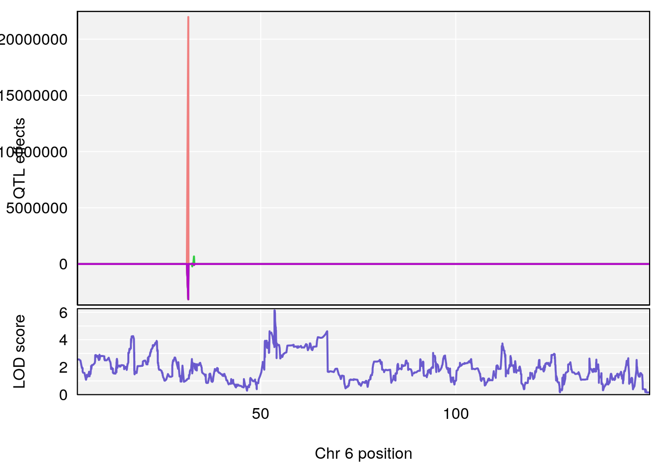
| Version | Author | Date |
|---|---|---|
| 9b57b94 | xhyuo | 2021-10-22 |
| Version | Author | Date |
|---|---|---|
| 9b57b94 | xhyuo | 2021-10-22 |
| Version | Author | Date |
|---|---|---|
| 9b57b94 | xhyuo | 2021-10-22 |
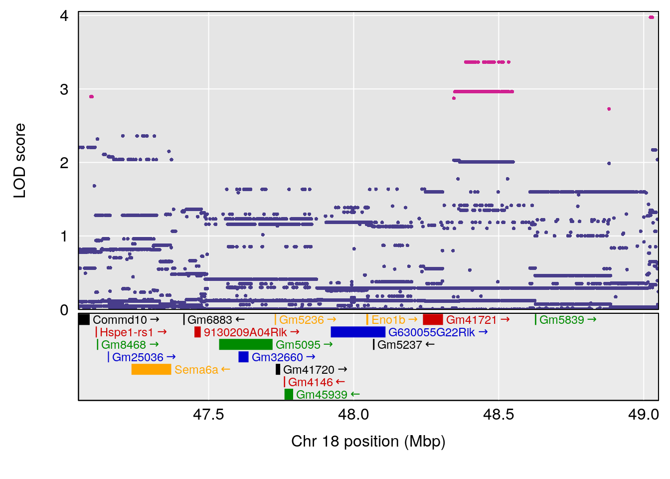
# [1] "Min.depression"
#   lodindex lodcolumn chr      pos     lod    ci_lo    ci_hi
# 1        1    pheno1   9 103.0599 6.78087 102.3457 103.0644
# [1] 1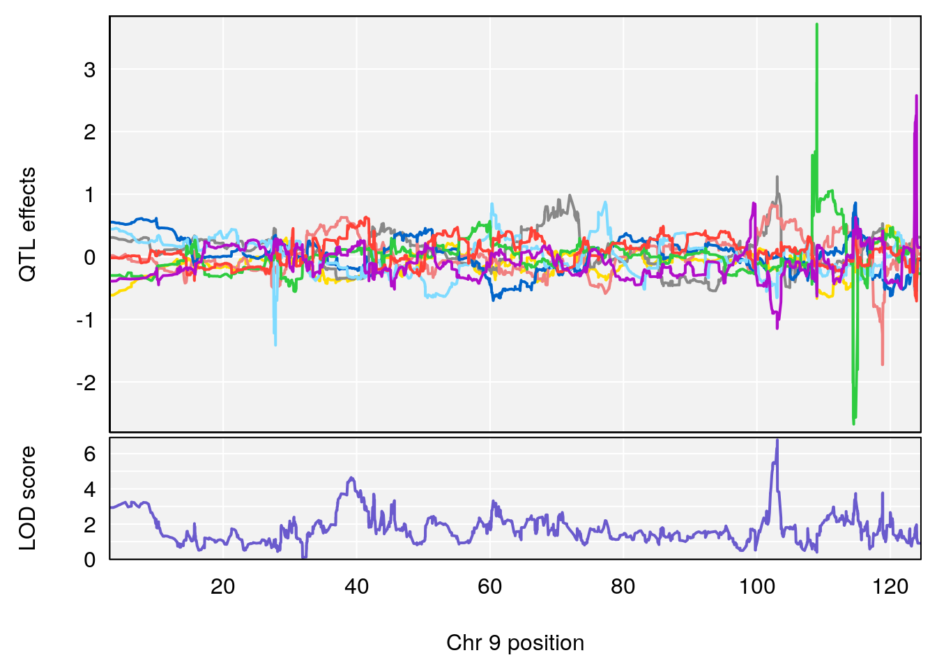
| Version | Author | Date |
|---|---|---|
| 9b57b94 | xhyuo | 2021-10-22 |
| Version | Author | Date |
|---|---|---|
| 9b57b94 | xhyuo | 2021-10-22 |
| Version | Author | Date |
|---|---|---|
| 9b57b94 | xhyuo | 2021-10-22 |
# [1] "Status_bin"
#   lodindex lodcolumn chr      pos      lod    ci_lo    ci_hi
# 1        1    pheno1  12 119.9713 7.062759  33.6258 120.1206
# 2        1    pheno1   X 166.3398 6.337632 164.4047 168.3021
# [1] 1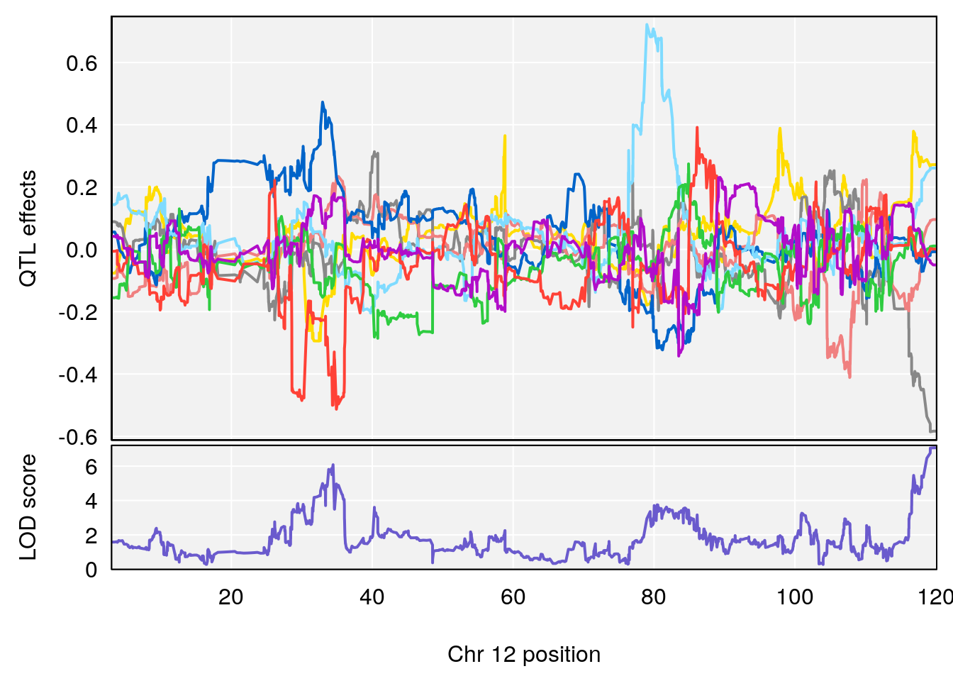
| Version | Author | Date |
|---|---|---|
| 9b57b94 | xhyuo | 2021-10-22 |
| Version | Author | Date |
|---|---|---|
| 9b57b94 | xhyuo | 2021-10-22 |
| Version | Author | Date |
|---|---|---|
| 9b57b94 | xhyuo | 2021-10-22 |
# [1] 2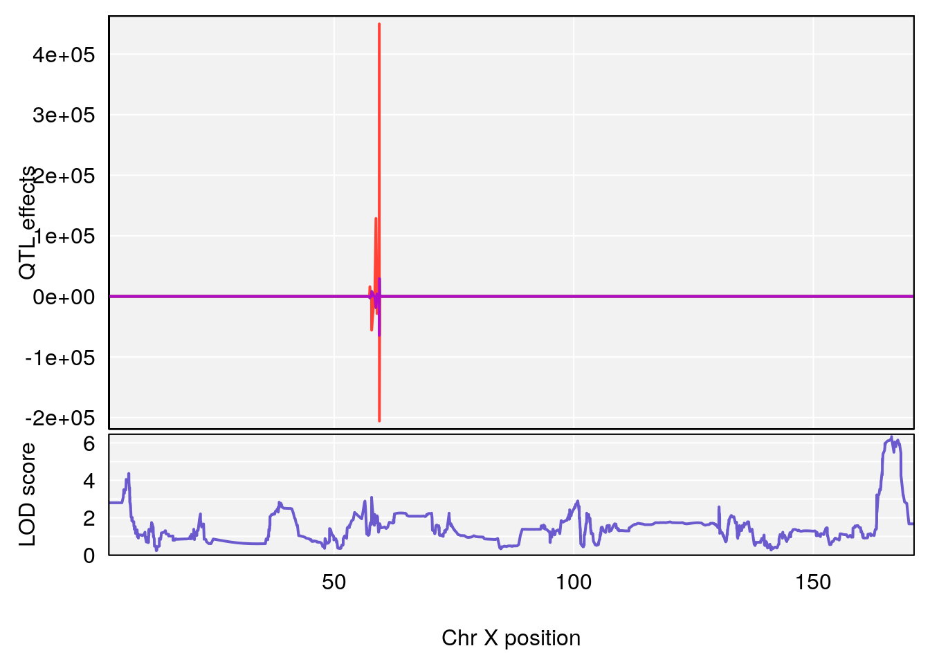
| Version | Author | Date |
|---|---|---|
| 9b57b94 | xhyuo | 2021-10-22 |
| Version | Author | Date |
|---|---|---|
| 9b57b94 | xhyuo | 2021-10-22 |
| Version | Author | Date |
|---|---|---|
| 9b57b94 | xhyuo | 2021-10-22 |
# [1] "f__Bpm"
#   lodindex lodcolumn chr      pos     lod    ci_lo   ci_hi
# 1        1    pheno1  18 14.50551 6.23671 13.51774 58.3684
# [1] 1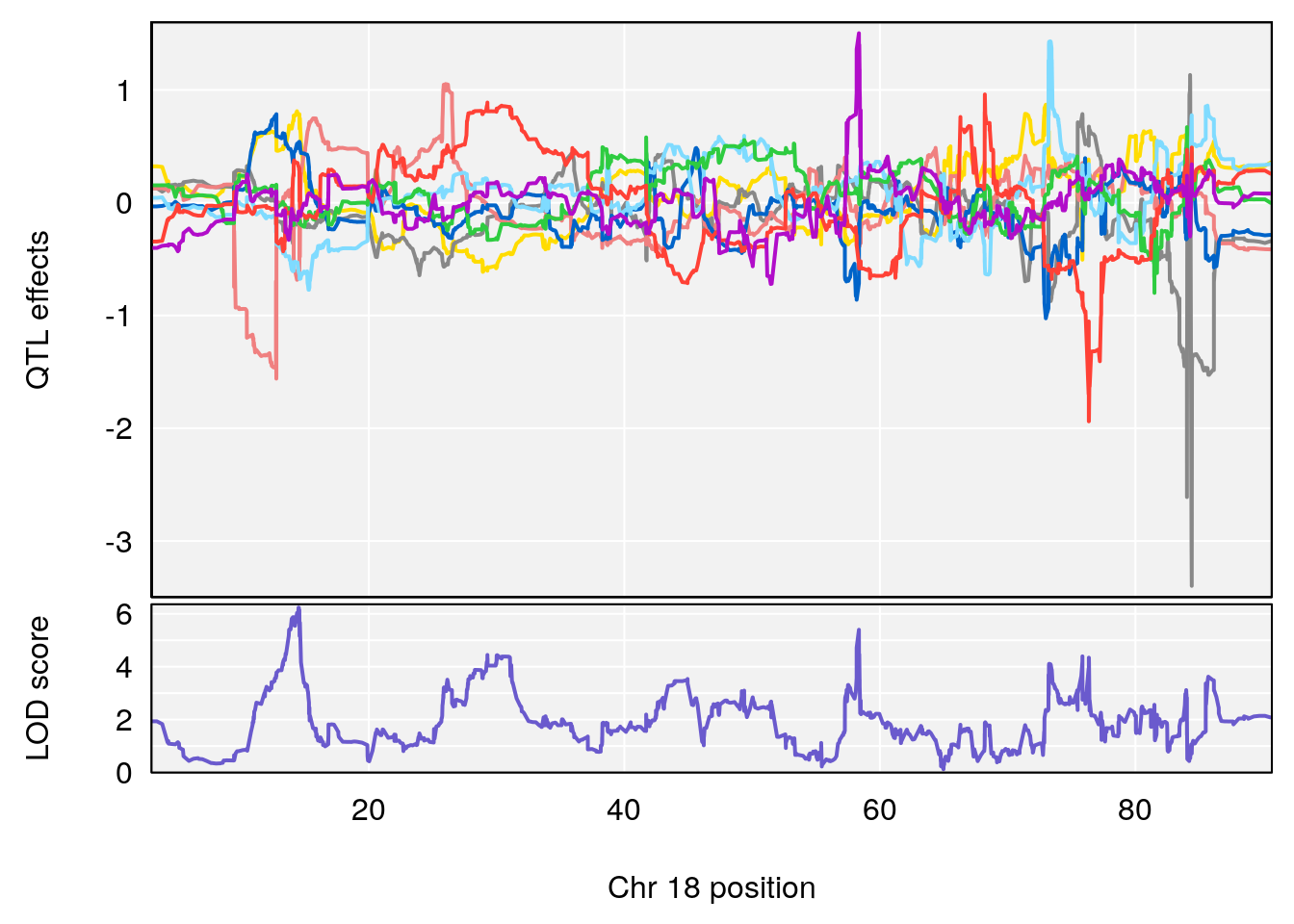
| Version | Author | Date |
|---|---|---|
| 9b57b94 | xhyuo | 2021-10-22 |
| Version | Author | Date |
|---|---|---|
| 9b57b94 | xhyuo | 2021-10-22 |
| Version | Author | Date |
|---|---|---|
| 9b57b94 | xhyuo | 2021-10-22 |
# [1] "TVb_ml"
#   lodindex lodcolumn chr       pos      lod     ci_lo     ci_hi
# 1        1    pheno1   1  30.99166 6.161079  25.51845  31.21353
# 2        1    pheno1  10 122.51450 6.507082 121.79792 122.82354
# 3        1    pheno1  18  48.05111 7.905729  46.96087  49.00996
# [1] 1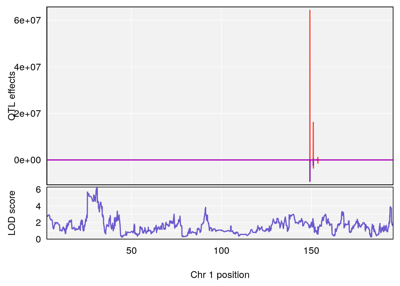
| Version | Author | Date |
|---|---|---|
| 9b57b94 | xhyuo | 2021-10-22 |
| Version | Author | Date |
|---|---|---|
| 9b57b94 | xhyuo | 2021-10-22 |
| Version | Author | Date |
|---|---|---|
| 9b57b94 | xhyuo | 2021-10-22 |
# [1] 2
| Version | Author | Date |
|---|---|---|
| 9b57b94 | xhyuo | 2021-10-22 |
| Version | Author | Date |
|---|---|---|
| 9b57b94 | xhyuo | 2021-10-22 |
| Version | Author | Date |
|---|---|---|
| 9b57b94 | xhyuo | 2021-10-22 |
# [1] 3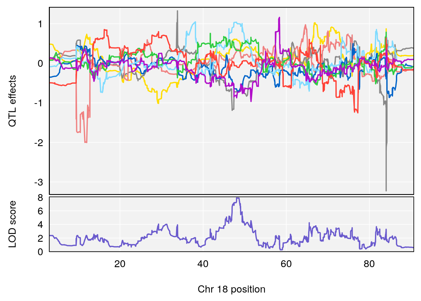
| Version | Author | Date |
|---|---|---|
| 9b57b94 | xhyuo | 2021-10-22 |
| Version | Author | Date |
|---|---|---|
| 9b57b94 | xhyuo | 2021-10-22 |
| Version | Author | Date |
|---|---|---|
| 9b57b94 | xhyuo | 2021-10-22 |
# [1] "MVb__ml_min"
# [1] lodindex lodcolumn chr pos lod ci_lo ci_hi
# <0 rows> (or 0-length row.names)
# [1] "Penh"
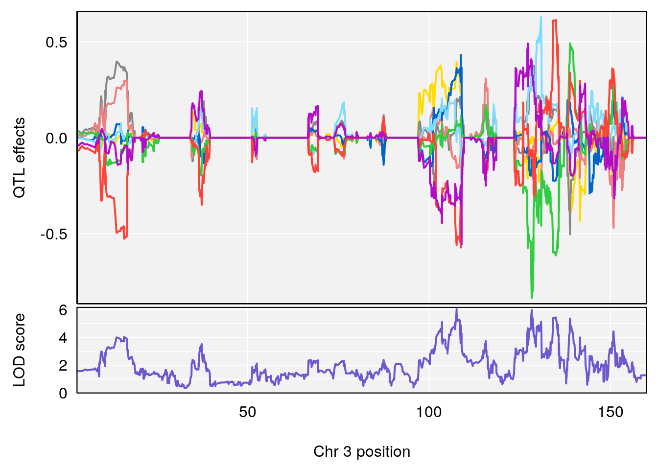
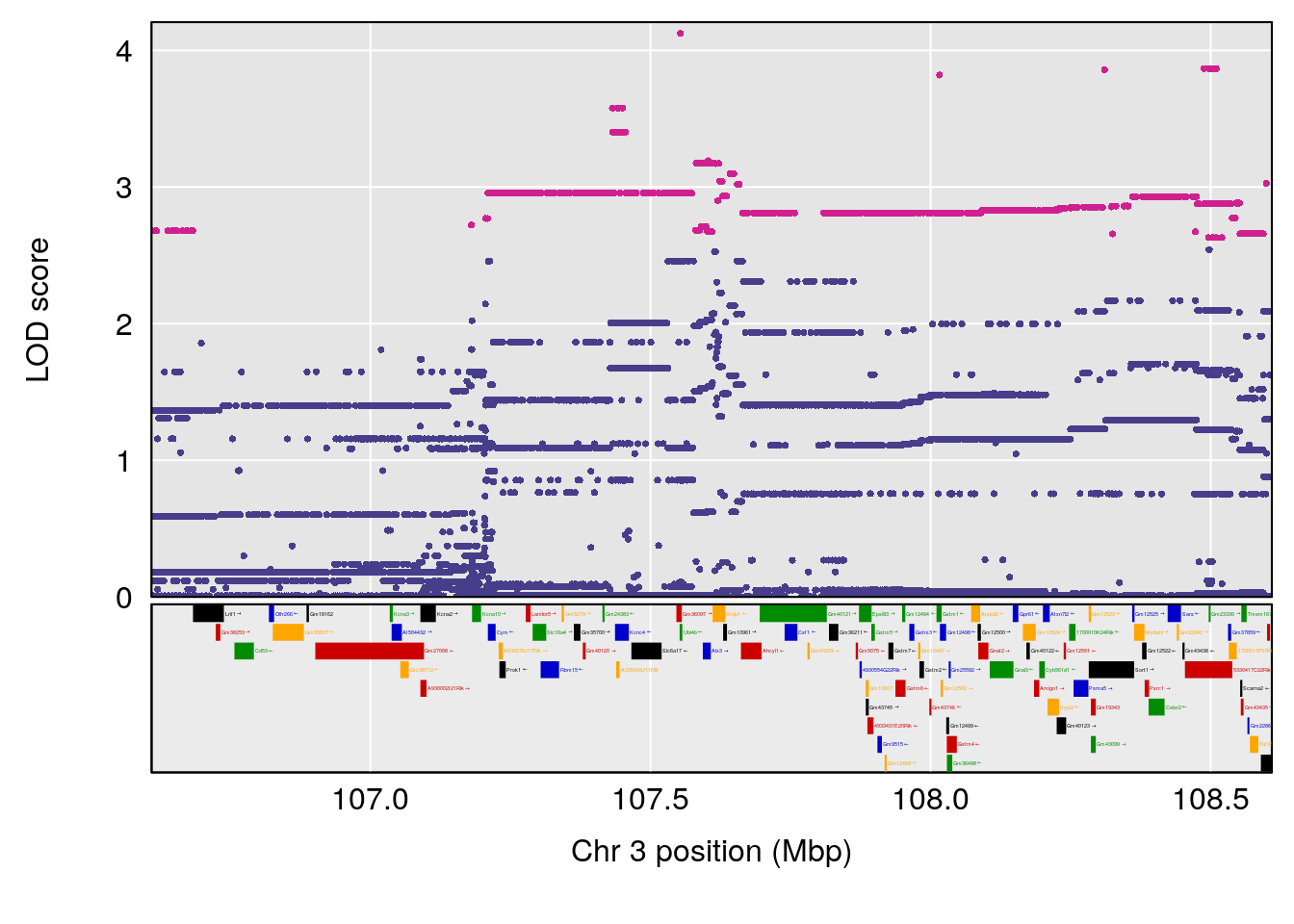
# lodindex lodcolumn chr pos lod ci_lo ci_hi
# 1 1 pheno1 3 107.60915 6.043981 103.05731 139.36271
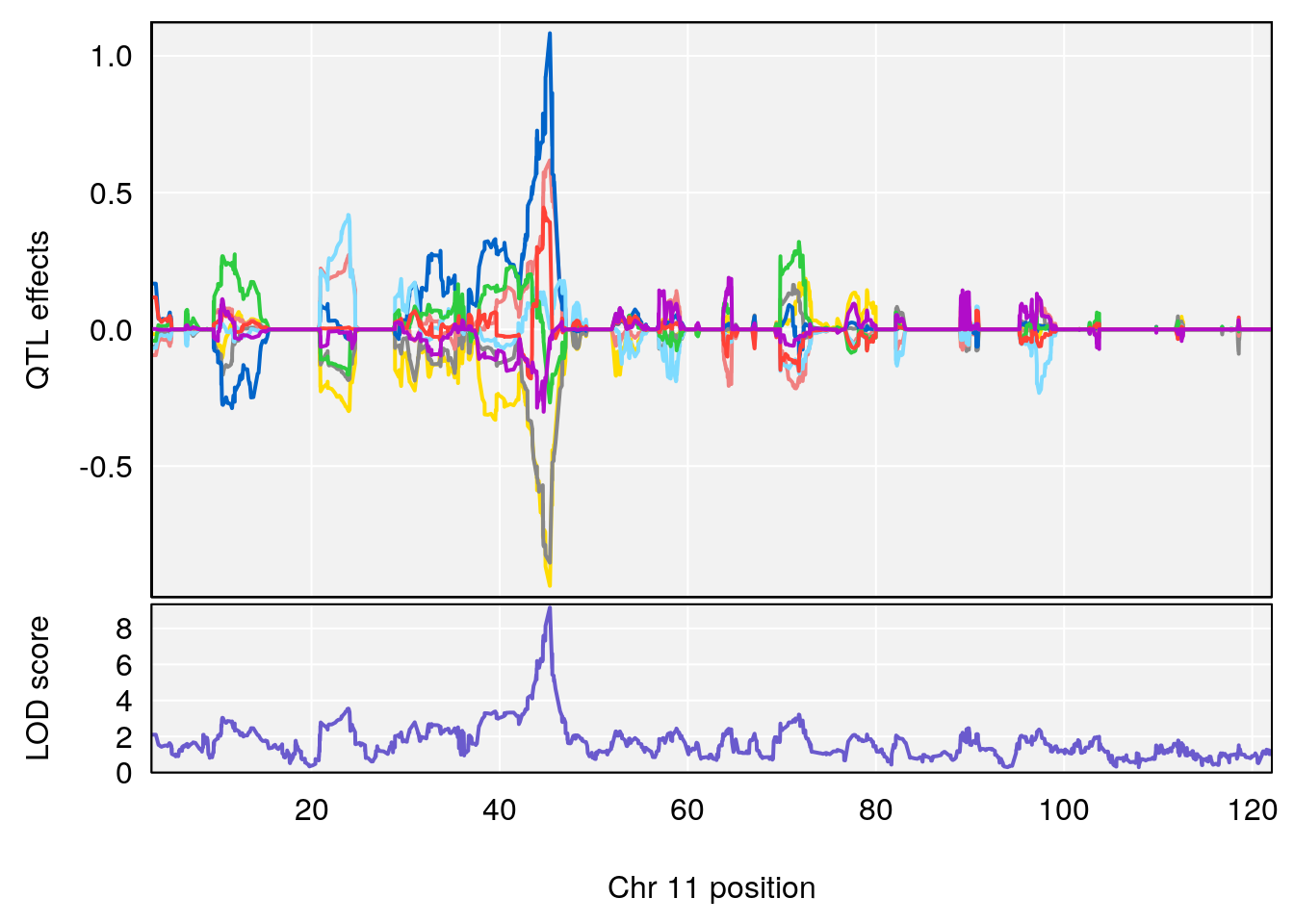
# 2 1 pheno1 11 45.34346 7.486808 44.59355 45.57867
# [1] 1
| Version | Author | Date |
|---|---|---|
| 9b57b94 | xhyuo | 2021-10-22 |
| Version | Author | Date |
|---|---|---|
| 9b57b94 | xhyuo | 2021-10-22 |
| Version | Author | Date |
|---|---|---|
| 9b57b94 | xhyuo | 2021-10-22 |
# [1] 2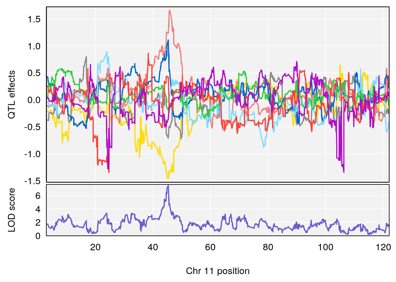
| Version | Author | Date |
|---|---|---|
| 9b57b94 | xhyuo | 2021-10-22 |

| Version | Author | Date |
|---|---|---|
| 9b57b94 | xhyuo | 2021-10-22 |
| Version | Author | Date |
|---|---|---|
| 9b57b94 | xhyuo | 2021-10-22 |
# [1] "PAU"
#   lodindex lodcolumn chr       pos      lod     ci_lo     ci_hi
# 1        1    pheno1   2  50.66047 6.103214  17.78081  65.34521
# 2        1    pheno1   3 134.94738 6.410510 129.58319 138.93596
# 3        1    pheno1  11  45.34346 9.286390  44.63365  45.57867
# [1] 1
| Version | Author | Date |
|---|---|---|
| 9b57b94 | xhyuo | 2021-10-22 |
| Version | Author | Date |
|---|---|---|
| 9b57b94 | xhyuo | 2021-10-22 |
| Version | Author | Date |
|---|---|---|
| 9b57b94 | xhyuo | 2021-10-22 |
# [1] 2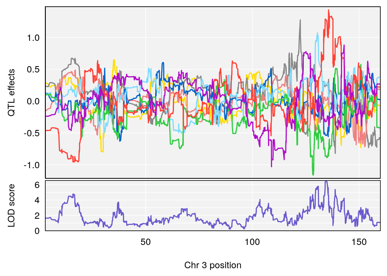
| Version | Author | Date |
|---|---|---|
| 9b57b94 | xhyuo | 2021-10-22 |
| Version | Author | Date |
|---|---|---|
| 9b57b94 | xhyuo | 2021-10-22 |
| Version | Author | Date |
|---|---|---|
| 9b57b94 | xhyuo | 2021-10-22 |
# [1] 3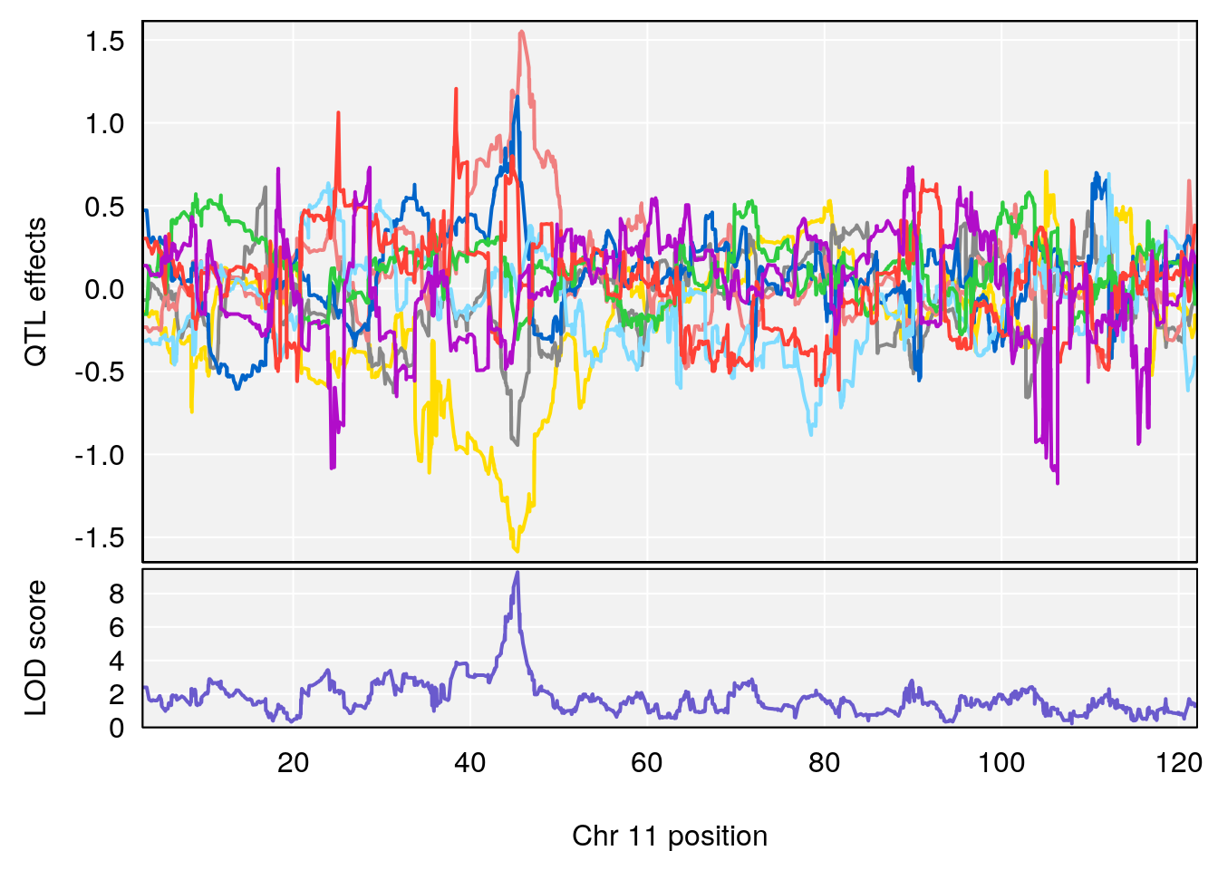
| Version | Author | Date |
|---|---|---|
| 9b57b94 | xhyuo | 2021-10-22 |
| Version | Author | Date |
|---|---|---|
| 9b57b94 | xhyuo | 2021-10-22 |
| Version | Author | Date |
|---|---|---|
| 9b57b94 | xhyuo | 2021-10-22 |
# [1] "Rpef"
#   lodindex lodcolumn chr       pos      lod    ci_lo    ci_hi
# 1        1    pheno1   1 40.980633 6.031467 40.80740 41.66614
# 2        1    pheno1   6 86.550595 6.075596 80.16050 87.75533
# 3        1    pheno1  15  5.436947 6.319855  3.00000 92.65671
# 4        1    pheno1   X 47.574474 7.068670 47.26218 47.97548
# [1] 1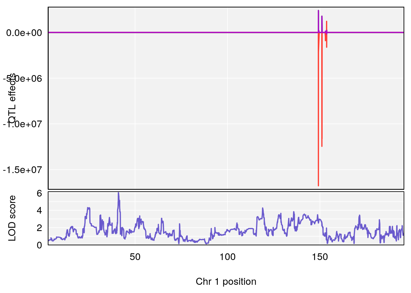
| Version | Author | Date |
|---|---|---|
| 9b57b94 | xhyuo | 2021-10-22 |
| Version | Author | Date |
|---|---|---|
| 9b57b94 | xhyuo | 2021-10-22 |
| Version | Author | Date |
|---|---|---|
| 9b57b94 | xhyuo | 2021-10-22 |
# [1] 2
| Version | Author | Date |
|---|---|---|
| 9b57b94 | xhyuo | 2021-10-22 |
| Version | Author | Date |
|---|---|---|
| 9b57b94 | xhyuo | 2021-10-22 |
| Version | Author | Date |
|---|---|---|
| 9b57b94 | xhyuo | 2021-10-22 |
# [1] 3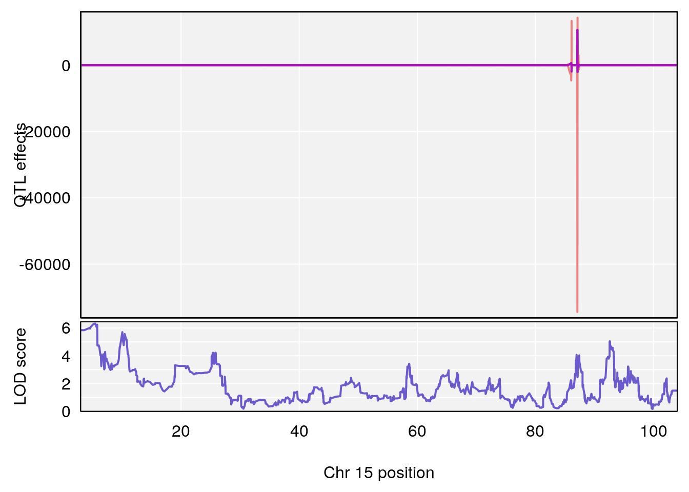
| Version | Author | Date |
|---|---|---|
| 9b57b94 | xhyuo | 2021-10-22 |
| Version | Author | Date |
|---|---|---|
| 9b57b94 | xhyuo | 2021-10-22 |
| Version | Author | Date |
|---|---|---|
| 9b57b94 | xhyuo | 2021-10-22 |
# [1] 4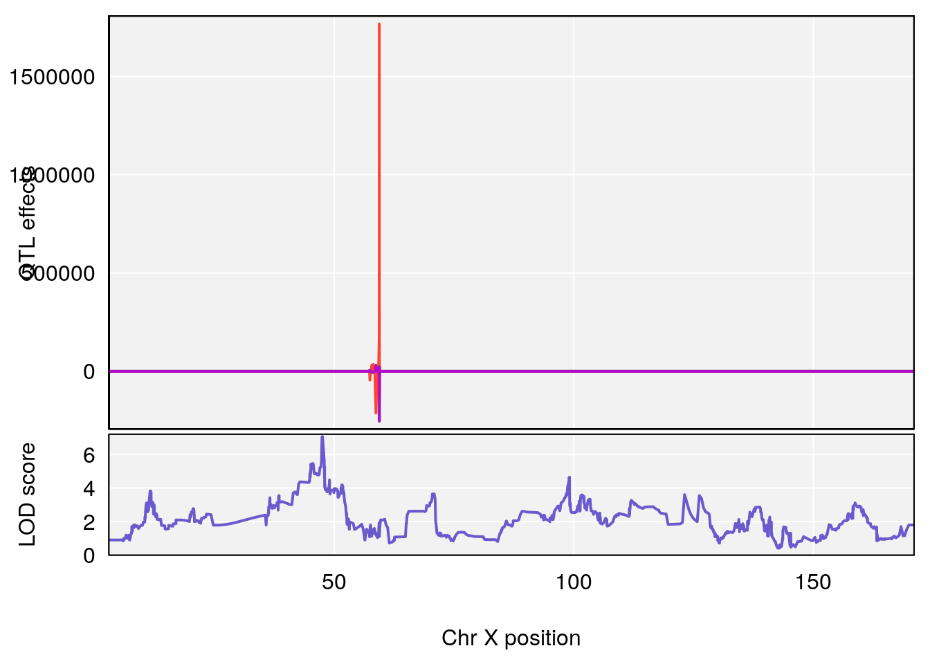
| Version | Author | Date |
|---|---|---|
| 9b57b94 | xhyuo | 2021-10-22 |
| Version | Author | Date |
|---|---|---|
| 9b57b94 | xhyuo | 2021-10-22 |
| Version | Author | Date |
|---|---|---|
| 9b57b94 | xhyuo | 2021-10-22 |
# [1] "PIFb"
#   lodindex lodcolumn chr      pos      lod    ci_lo   ci_hi
# 1        1    pheno1  18 48.06477 6.126548 28.94452 58.3684
# [1] 1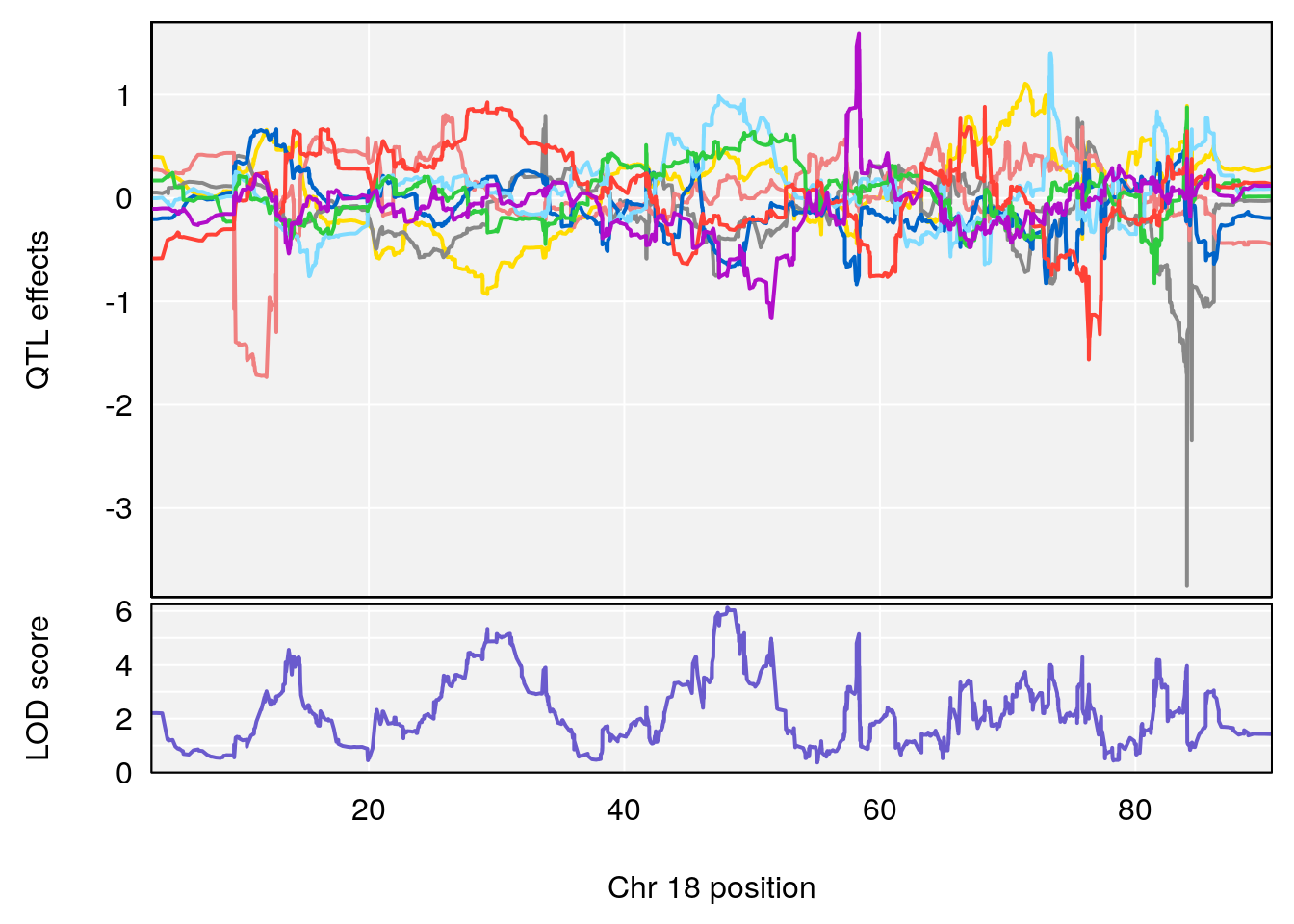
| Version | Author | Date |
|---|---|---|
| 9b57b94 | xhyuo | 2021-10-22 |
| Version | Author | Date |
|---|---|---|
| 9b57b94 | xhyuo | 2021-10-22 |
| Version | Author | Date |
|---|---|---|
| 9b57b94 | xhyuo | 2021-10-22 |
# [1] "PEFb"
# [1] lodindex  lodcolumn chr       pos       lod       ci_lo     ci_hi
# <0 rows> (or 0-length row.names)
# [1] "Ti__sec"
#   lodindex lodcolumn chr      pos      lod   ci_lo    ci_hi
# 1        1    pheno1   X 47.46421 6.146712 45.1181 51.89095
# [1] 1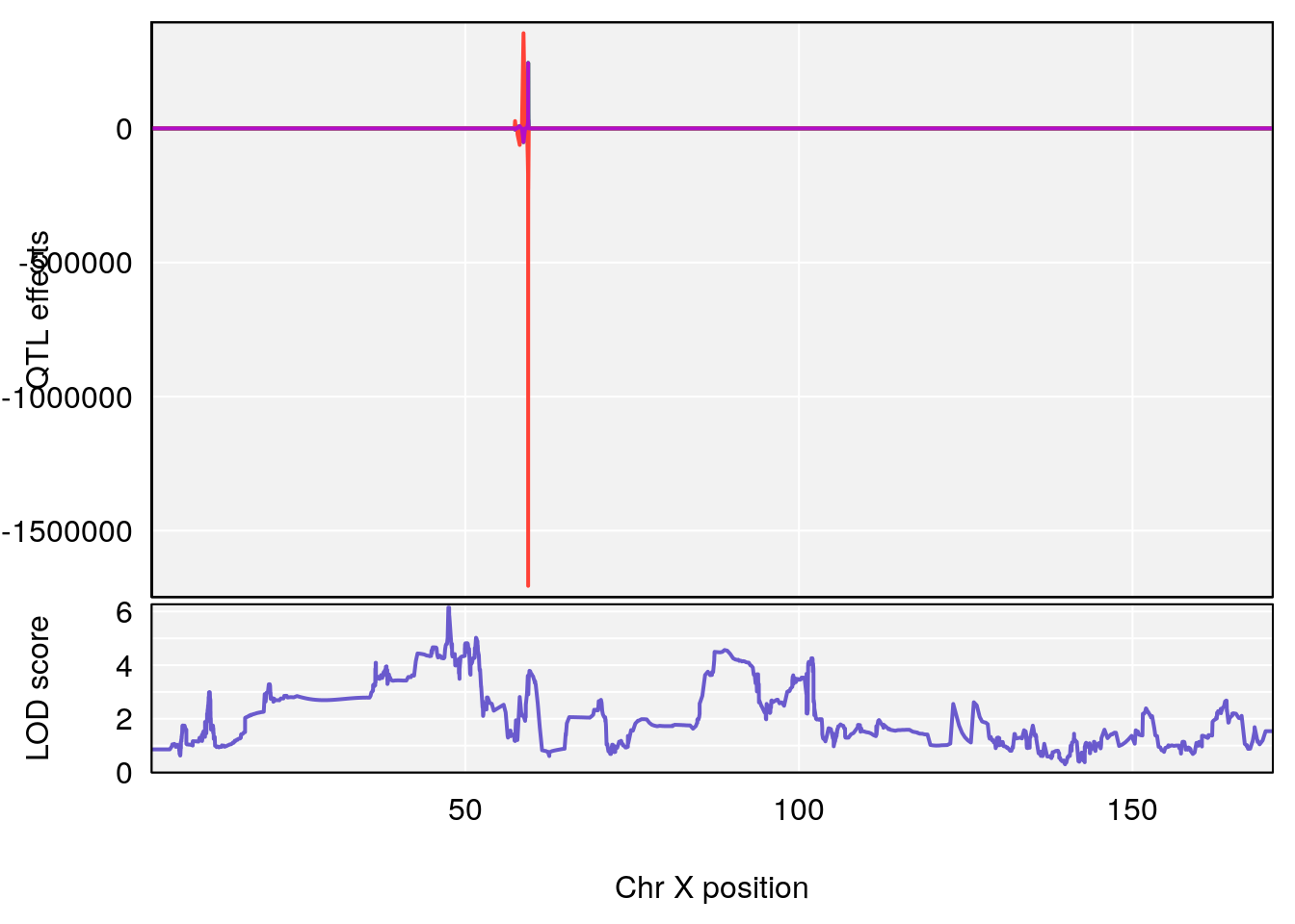
| Version | Author | Date |
|---|---|---|
| 9b57b94 | xhyuo | 2021-10-22 |
| Version | Author | Date |
|---|---|---|
| 9b57b94 | xhyuo | 2021-10-22 |
| Version | Author | Date |
|---|---|---|
| 9b57b94 | xhyuo | 2021-10-22 |
# [1] "Te__sec"
#   lodindex lodcolumn chr      pos      lod    ci_lo    ci_hi
# 1        1    pheno1  18 14.52647 6.280781 13.51774 58.36840
# 2        1    pheno1   X 47.57447 6.096542 45.11810 48.17457
# [1] 1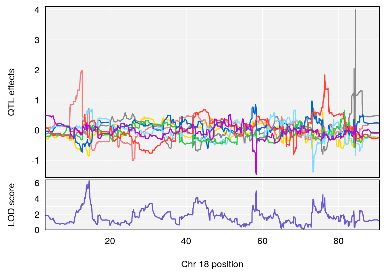
| Version | Author | Date |
|---|---|---|
| 9b57b94 | xhyuo | 2021-10-22 |
| Version | Author | Date |
|---|---|---|
| 9b57b94 | xhyuo | 2021-10-22 |
| Version | Author | Date |
|---|---|---|
| 9b57b94 | xhyuo | 2021-10-22 |
# [1] 2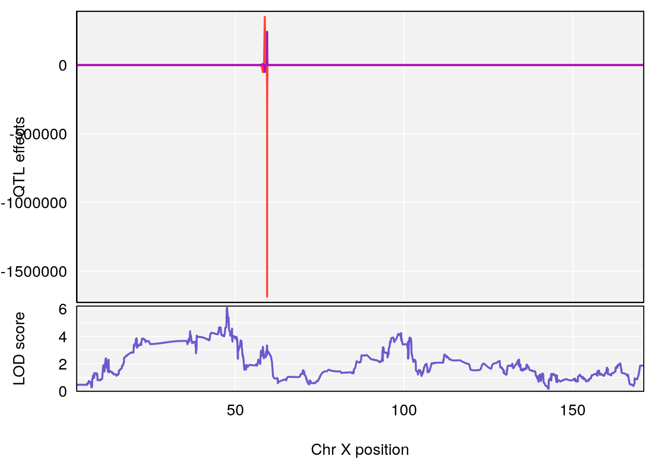
| Version | Author | Date |
|---|---|---|
| 9b57b94 | xhyuo | 2021-10-22 |
| Version | Author | Date |
|---|---|---|
| 9b57b94 | xhyuo | 2021-10-22 |
| Version | Author | Date |
|---|---|---|
| 9b57b94 | xhyuo | 2021-10-22 |
# [1] "EF50"
# [1] lodindex  lodcolumn chr       pos       lod       ci_lo     ci_hi
# <0 rows> (or 0-length row.names)
# [1] "EIP__ms"
#   lodindex lodcolumn chr      pos      lod    ci_lo    ci_hi
# 1        1    pheno1  12 75.10641 6.272502 73.22861 75.16873
# 2        1    pheno1   X 98.98553 7.709884 47.35806 99.12447
# [1] 1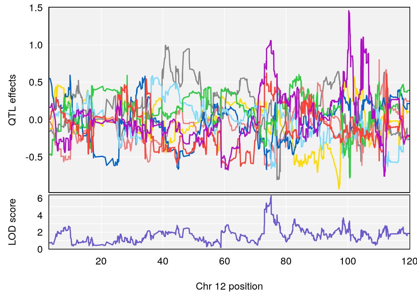
| Version | Author | Date |
|---|---|---|
| 9b57b94 | xhyuo | 2021-10-22 |
| Version | Author | Date |
|---|---|---|
| 9b57b94 | xhyuo | 2021-10-22 |
| Version | Author | Date |
|---|---|---|
| 9b57b94 | xhyuo | 2021-10-22 |
# [1] 2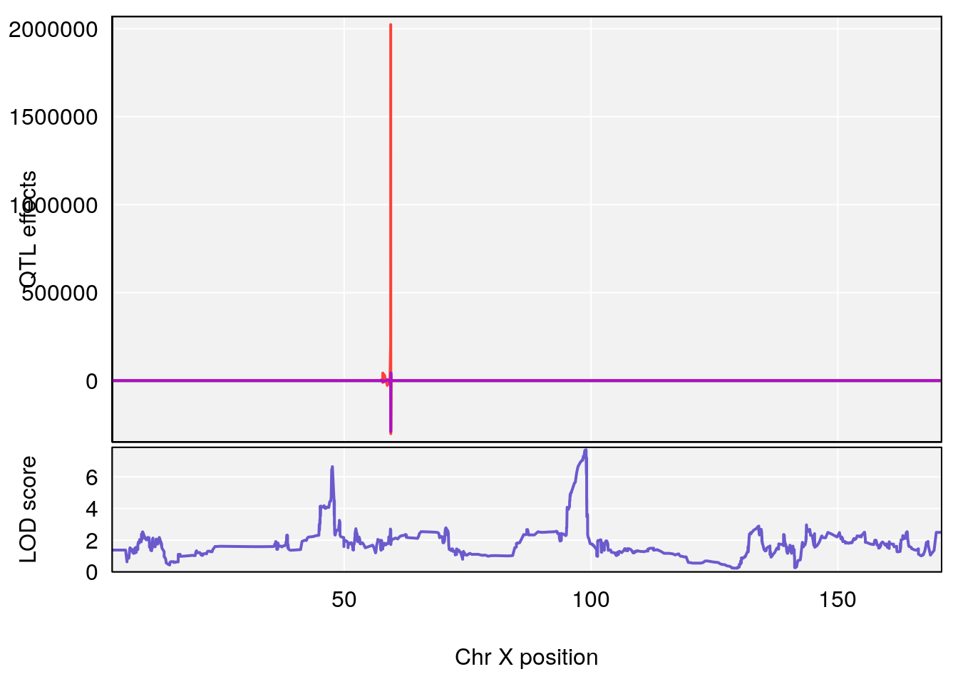
| Version | Author | Date |
|---|---|---|
| 9b57b94 | xhyuo | 2021-10-22 |
| Version | Author | Date |
|---|---|---|
| 9b57b94 | xhyuo | 2021-10-22 |
| Version | Author | Date |
|---|---|---|
| 9b57b94 | xhyuo | 2021-10-22 |
# [1] "EEP_9ms"
#   lodindex lodcolumn chr      pos      lod    ci_lo    ci_hi
# 1        1    pheno1   4 30.64705 6.038384 28.85145 31.62183
# 2        1    pheno1  11 88.95060 6.170713 88.66966 89.32368
# 3        1    pheno1  15 97.55762 6.054756 97.40095 98.56295
# 4        1    pheno1  18 13.96979 6.138380 10.48923 14.12114
# [1] 1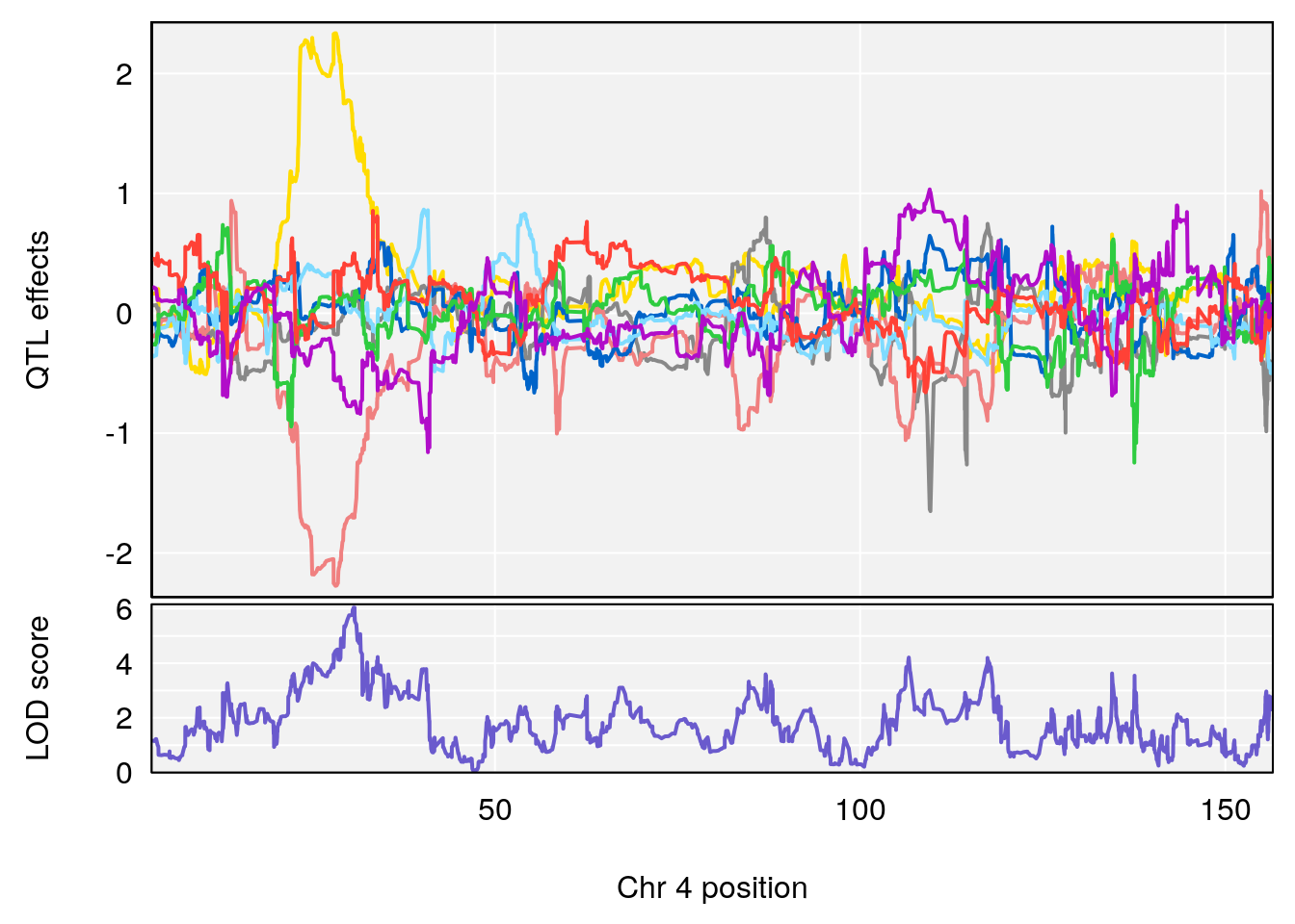
| Version | Author | Date |
|---|---|---|
| 9b57b94 | xhyuo | 2021-10-22 |
| Version | Author | Date |
|---|---|---|
| 9b57b94 | xhyuo | 2021-10-22 |
| Version | Author | Date |
|---|---|---|
| 9b57b94 | xhyuo | 2021-10-22 |
# [1] 2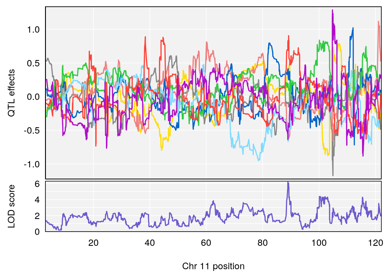
| Version | Author | Date |
|---|---|---|
| 9b57b94 | xhyuo | 2021-10-22 |
| Version | Author | Date |
|---|---|---|
| 9b57b94 | xhyuo | 2021-10-22 |
| Version | Author | Date |
|---|---|---|
| 9b57b94 | xhyuo | 2021-10-22 |
# [1] 3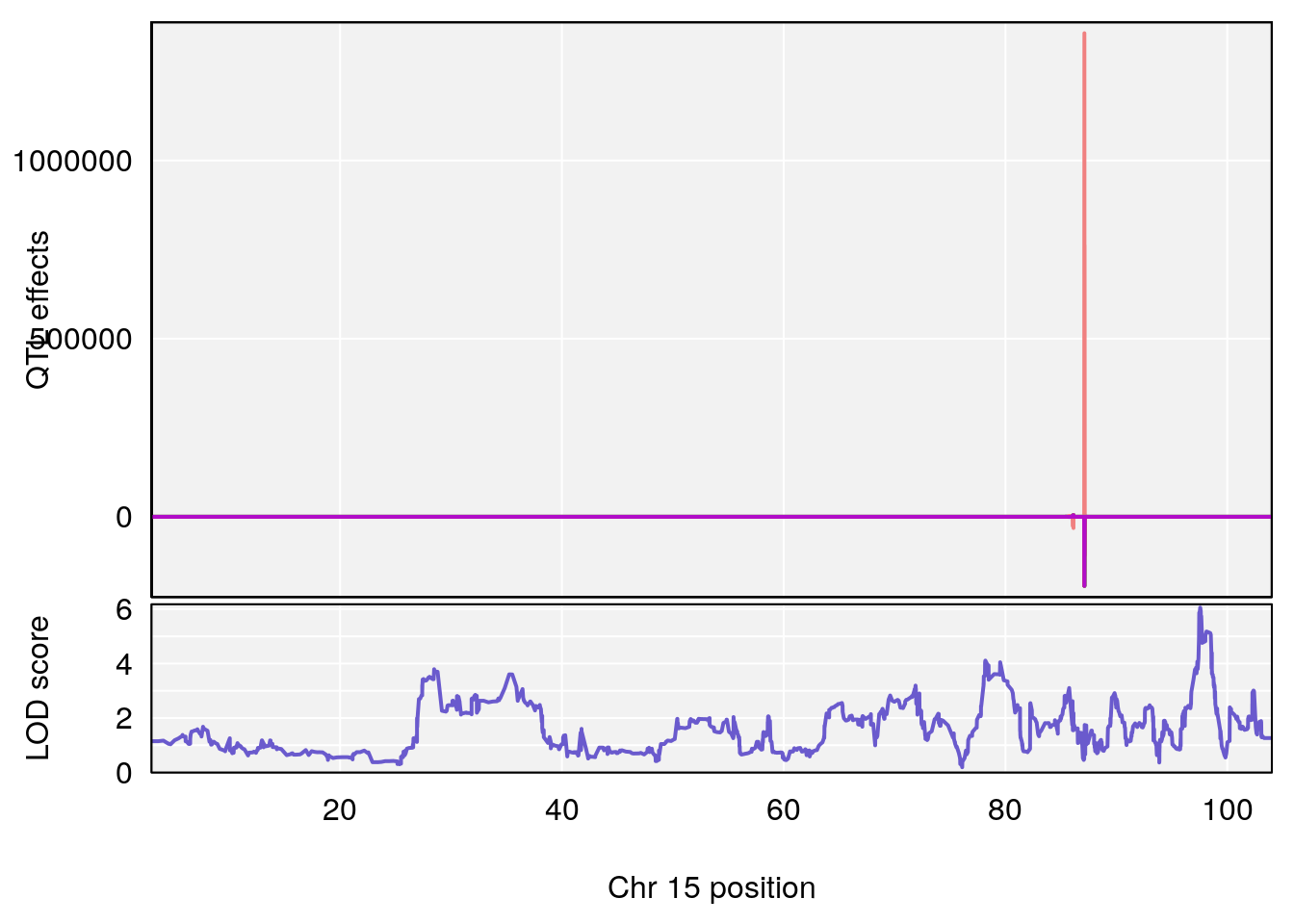
| Version | Author | Date |
|---|---|---|
| 9b57b94 | xhyuo | 2021-10-22 |
| Version | Author | Date |
|---|---|---|
| 9b57b94 | xhyuo | 2021-10-22 |
| Version | Author | Date |
|---|---|---|
| 9b57b94 | xhyuo | 2021-10-22 |
# [1] 4
| Version | Author | Date |
|---|---|---|
| 9b57b94 | xhyuo | 2021-10-22 |
| Version | Author | Date |
|---|---|---|
| 9b57b94 | xhyuo | 2021-10-22 |
| Version | Author | Date |
|---|---|---|
| 9b57b94 | xhyuo | 2021-10-22 |
# [1] "Tr__sec"
# [1] lodindex  lodcolumn chr       pos       lod       ci_lo     ci_hi
# <0 rows> (or 0-length row.names)
# [1] "TB"
#   lodindex lodcolumn chr      pos      lod    ci_lo    ci_hi
# 1        1    pheno1  17 51.97762 6.019379 51.49180 54.66990
# 2        1    pheno1   X 47.57447 7.796565 47.26218 47.90373
# [1] 1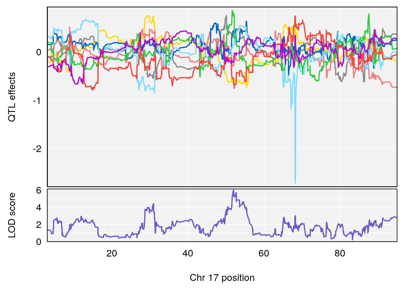
| Version | Author | Date |
|---|---|---|
| 9b57b94 | xhyuo | 2021-10-22 |
| Version | Author | Date |
|---|---|---|
| 9b57b94 | xhyuo | 2021-10-22 |
| Version | Author | Date |
|---|---|---|
| 9b57b94 | xhyuo | 2021-10-22 |
# [1] 2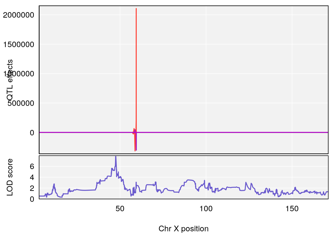
| Version | Author | Date |
|---|---|---|
| 9b57b94 | xhyuo | 2021-10-22 |
| Version | Author | Date |
|---|---|---|
| 9b57b94 | xhyuo | 2021-10-22 |
| Version | Author | Date |
|---|---|---|
| 9b57b94 | xhyuo | 2021-10-22 |
# [1] "TP"
#   lodindex lodcolumn chr      pos      lod    ci_lo    ci_hi
# 1        1    pheno1  11 45.34637 9.159164 44.84433 45.57867
# 2        1    pheno1  12 76.39568 6.204830 75.10641 77.00632
# [1] 1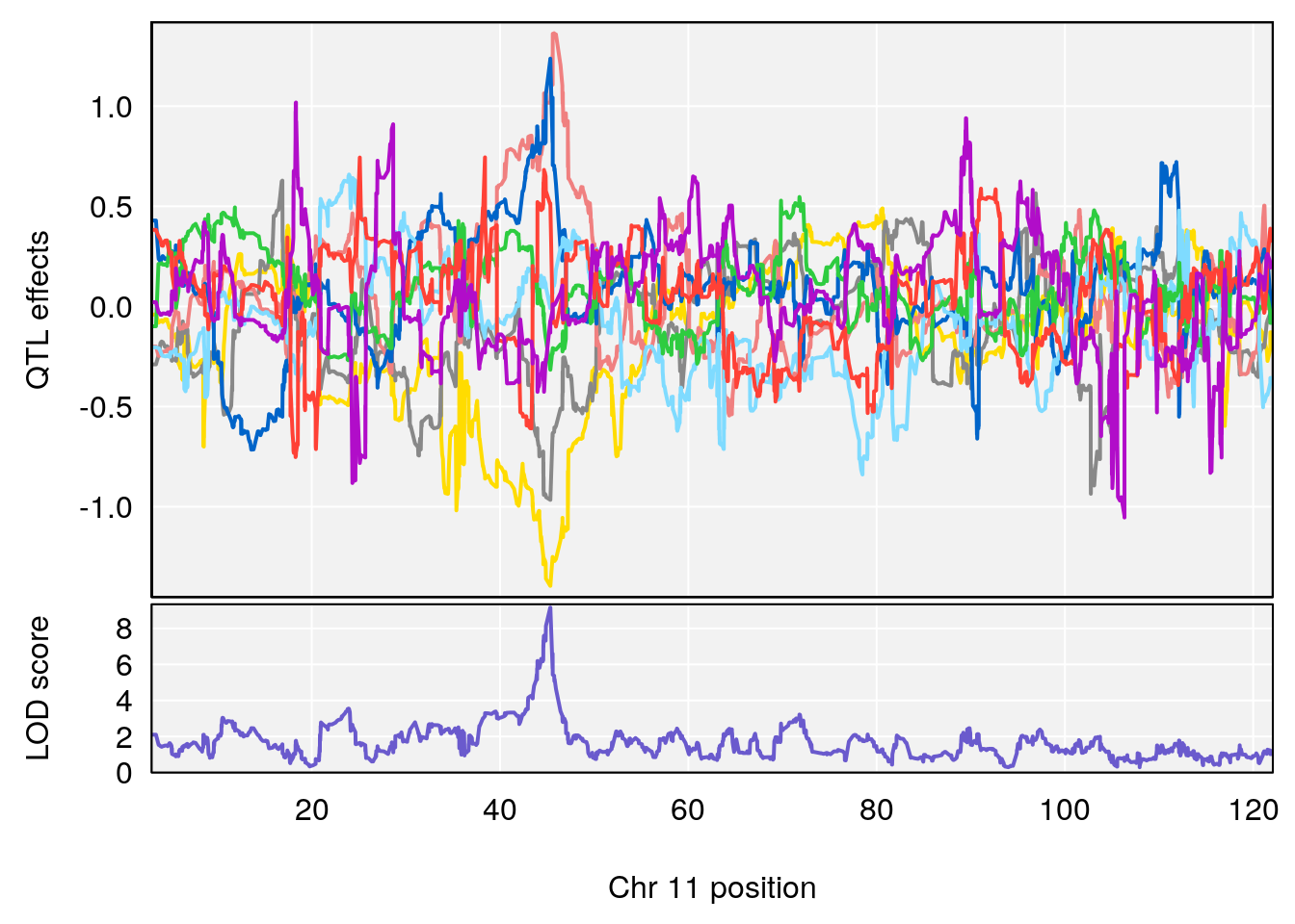
| Version | Author | Date |
|---|---|---|
| 9b57b94 | xhyuo | 2021-10-22 |
| Version | Author | Date |
|---|---|---|
| 9b57b94 | xhyuo | 2021-10-22 |
| Version | Author | Date |
|---|---|---|
| 9b57b94 | xhyuo | 2021-10-22 |
# [1] 2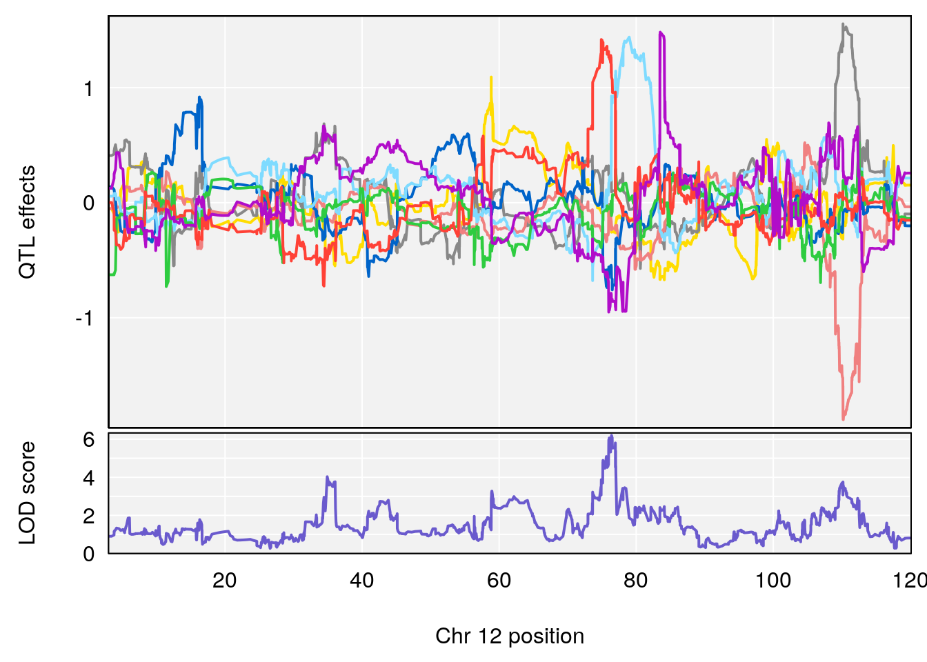
| Version | Author | Date |
|---|---|---|
| 9b57b94 | xhyuo | 2021-10-22 |

| Version | Author | Date |
|---|---|---|
| 9b57b94 | xhyuo | 2021-10-22 |
| Version | Author | Date |
|---|---|---|
| 9b57b94 | xhyuo | 2021-10-22 |
# [1] "Rinx"
#   lodindex lodcolumn chr      pos     lod    ci_lo    ci_hi
# 1        1    pheno1   X 47.46421 9.65094 47.35806 47.90373
# [1] 1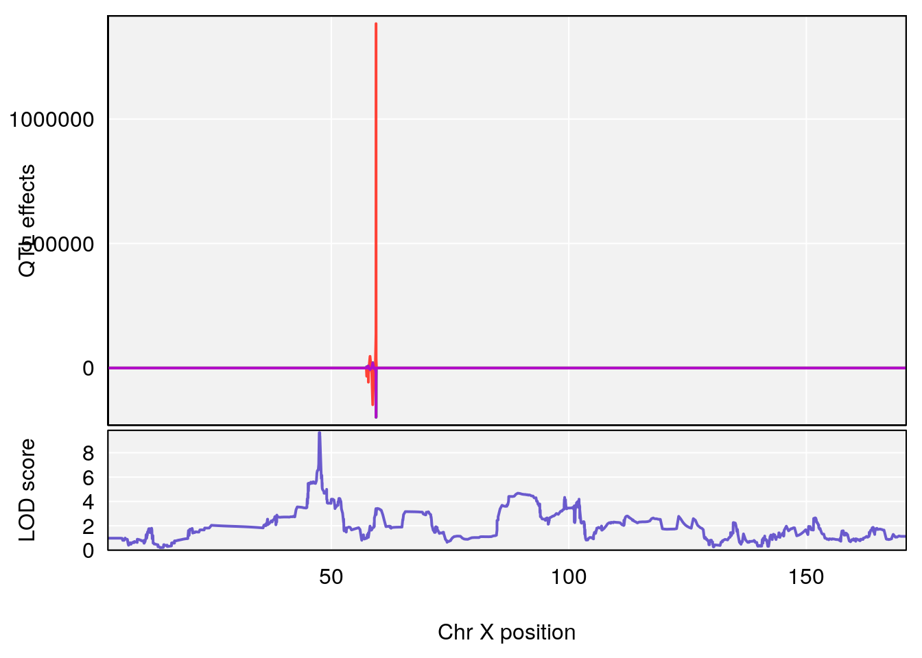
| Version | Author | Date |
|---|---|---|
| 9b57b94 | xhyuo | 2021-10-22 |
| Version | Author | Date |
|---|---|---|
| 9b57b94 | xhyuo | 2021-10-22 |
| Version | Author | Date |
|---|---|---|
| 9b57b94 | xhyuo | 2021-10-22 |
# [1] "Ttot"
# [1] lodindex  lodcolumn chr       pos       lod       ci_lo     ci_hi
# <0 rows> (or 0-length row.names)
# [1] "duty_cycle"
#   lodindex lodcolumn chr      pos      lod    ci_lo     ci_hi
# 1        1    pheno1   1 14.58271 6.484326 14.26449  45.04740
# 2        1    pheno1   7 61.28043 6.095969 57.52944 138.63371
# 3        1    pheno1  12 77.02882 6.168584 76.96394  78.03074
# 4        1    pheno1  17 37.06944 6.465960 36.27663  54.24285
# [1] 1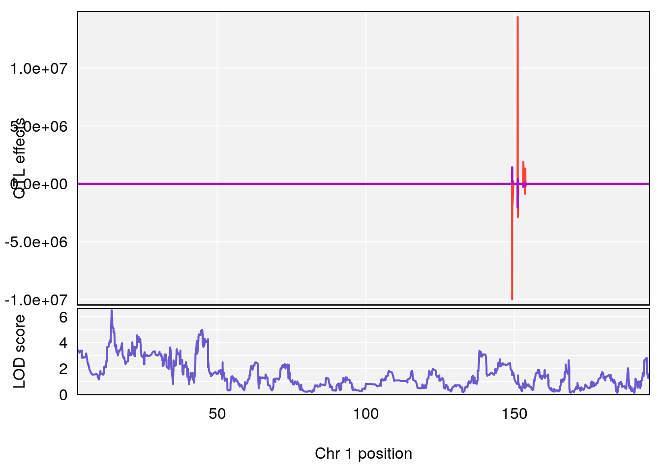
| Version | Author | Date |
|---|---|---|
| 9b57b94 | xhyuo | 2021-10-22 |
| Version | Author | Date |
|---|---|---|
| 9b57b94 | xhyuo | 2021-10-22 |
| Version | Author | Date |
|---|---|---|
| 9b57b94 | xhyuo | 2021-10-22 |
# [1] 2
| Version | Author | Date |
|---|---|---|
| 9b57b94 | xhyuo | 2021-10-22 |
| Version | Author | Date |
|---|---|---|
| 9b57b94 | xhyuo | 2021-10-22 |
| Version | Author | Date |
|---|---|---|
| 9b57b94 | xhyuo | 2021-10-22 |
# [1] 3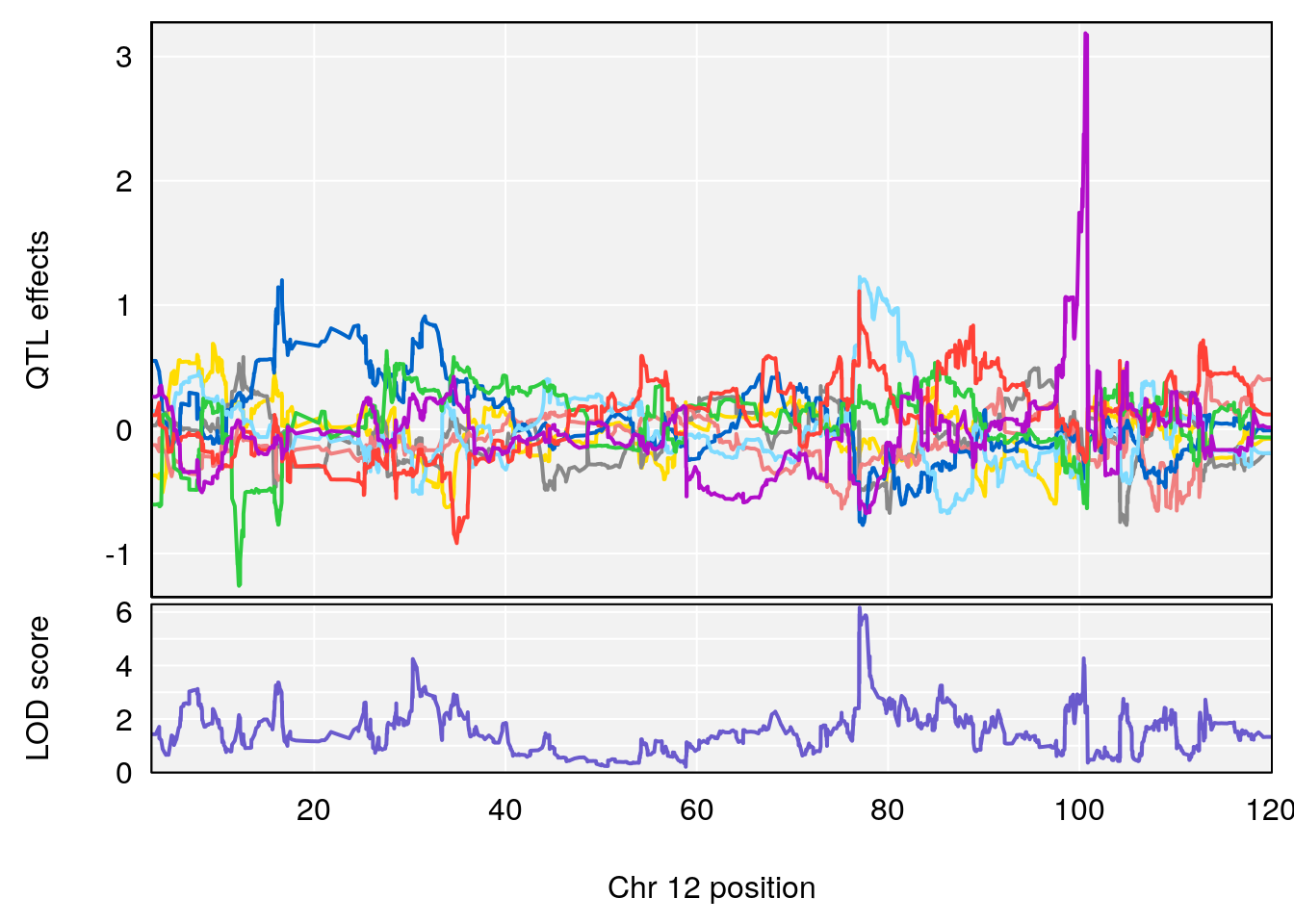
| Version | Author | Date |
|---|---|---|
| 9b57b94 | xhyuo | 2021-10-22 |
| Version | Author | Date |
|---|---|---|
| 9b57b94 | xhyuo | 2021-10-22 |
| Version | Author | Date |
|---|---|---|
| 9b57b94 | xhyuo | 2021-10-22 |
# [1] 4
| Version | Author | Date |
|---|---|---|
| 9b57b94 | xhyuo | 2021-10-22 |
| Version | Author | Date |
|---|---|---|
| 9b57b94 | xhyuo | 2021-10-22 |
| Version | Author | Date |
|---|---|---|
| 9b57b94 | xhyuo | 2021-10-22 |
# [1] "resp_flow"
# [1] lodindex  lodcolumn chr       pos       lod       ci_lo     ci_hi
# <0 rows> (or 0-length row.names)
# [1] "insp_flow"
#   lodindex lodcolumn chr      pos      lod     ci_lo    ci_hi
# 1        1    pheno1  17 55.28882 6.099506  5.565477 56.03294
# 2        1    pheno1  18 48.06477 6.187377 29.173138 51.95635
# [1] 1
| Version | Author | Date |
|---|---|---|
| 3f3ae81 | xhyuo | 2021-11-15 |
| Version | Author | Date |
|---|---|---|
| 3f3ae81 | xhyuo | 2021-11-15 |
| Version | Author | Date |
|---|---|---|
| 3f3ae81 | xhyuo | 2021-11-15 |
# [1] 2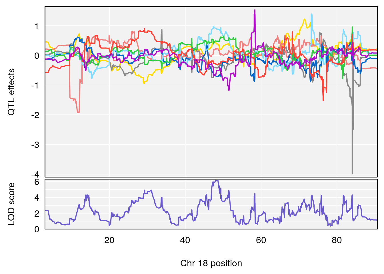
| Version | Author | Date |
|---|---|---|
| 3f3ae81 | xhyuo | 2021-11-15 |
| Version | Author | Date |
|---|---|---|
| 3f3ae81 | xhyuo | 2021-11-15 |
| Version | Author | Date |
|---|---|---|
| 3f3ae81 | xhyuo | 2021-11-15 |
# [1] "exp_flow"
# [1] lodindex lodcolumn chr pos lod ci_lo ci_hi
# <0 rows> (or 0-length row.names)
#save peaks coeff plot
for(i in names(qtl.morphine.out)){
print(i)
peaks <- find_peaks(qtl.morphine.out[[i]], map=pmap, threshold=6, drop=1.5)
fname <- paste("output/Fentanyl/DO_fentanyl_69k_",i,"_coefplot.pdf",sep="")
pdf(file = fname, width = 16, height =8)
if(dim(peaks)[1] != 0){
for(p in 1:dim(peaks)[1]) {
print(p)
chr <-peaks[p,3]
#coeff plot
par(mar=c(4.1, 4.1, 0.6, 0.6))
plot_coefCC(coef_c1[[i]][[p]], pmap[chr], scan1_output=qtl.morphine.out[[i]], bgcolor="gray95", legend=NULL)
plot(out_snps[[i]][[p]]$lod, out_snps[[i]][[p]]$snpinfo, drop_hilit=1.5, genes=out_genes[[i]][[p]])
}
}
dev.off()
}
# [1] "Survival.Time"
# [1] 1
# [1] "Recovery.Time"
# [1] 1
# [1] "Min.depression"
# [1] 1
# [1] "Status_bin"
# [1] 1
# [1] 2
# [1] "f__Bpm"
# [1] 1
# [1] "TVb_ml"
# [1] 1
# [1] 2
# [1] 3
# [1] "MVb__ml_min"
# [1] "Penh"
# [1] 1
# [1] 2
# [1] "PAU"
# [1] 1
# [1] 2
# [1] 3
# [1] "Rpef"
# [1] 1
# [1] 2
# [1] 3
# [1] 4
# [1] "PIFb"
# [1] 1
# [1] "PEFb"
# [1] "Ti__sec"
# [1] 1
# [1] "Te__sec"
# [1] 1
# [1] 2
# [1] "EF50"
# [1] "EIP__ms"
# [1] 1
# [1] 2
# [1] "EEP_9ms"
# [1] 1
# [1] 2
# [1] 3
# [1] 4
# [1] "Tr__sec"
# [1] "TB"
# [1] 1
# [1] 2
# [1] "TP"
# [1] 1
# [1] 2
# [1] "Rinx"
# [1] 1
# [1] "Ttot"
# [1] "duty_cycle"
# [1] 1
# [1] 2
# [1] 3
# [1] 4
# [1] "resp_flow"
# [1] "insp_flow"
# [1] 1
# [1] 2
# [1] "exp_flow"
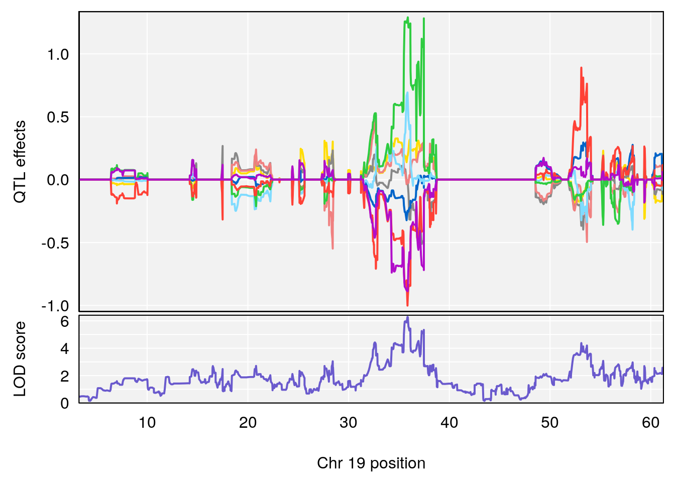
#save peaks coeff blup plot
for(i in names(qtl.morphine.out)){
print(i)
peaks <- find_peaks(qtl.morphine.out[[i]], map=pmap, threshold=6, drop=1.5)
fname <- paste("output/Fentanyl/DO_fentanyl_69k_",i,"_coefplot_blup.pdf",sep="")
pdf(file = fname, width = 16, height =8)
if(dim(peaks)[1] != 0){
for(p in 1:dim(peaks)[1]) {
print(p)
chr <-peaks[p,3]
#coeff plot
par(mar=c(4.1, 4.1, 0.6, 0.6))
plot_coefCC(coef_c2[[i]][[p]], pmap[chr], scan1_output=qtl.morphine.out[[i]], bgcolor="gray95", legend=NULL)
plot(out_snps[[i]][[p]]$lod, out_snps[[i]][[p]]$snpinfo, drop_hilit=1.5, genes=out_genes[[i]][[p]])
}
}
dev.off()
}
# [1] "Survival.Time"
# [1] 1
# [1] "Recovery.Time"
# [1] 1
# [1] "Min.depression"
# [1] 1
# [1] "Status_bin"
# [1] 1
# [1] 2
# [1] "f__Bpm"
# [1] 1
# [1] "TVb_ml"
# [1] 1
# [1] 2
# [1] 3
# [1] "MVb__ml_min"
# [1] "Penh"
# [1] 1
# [1] 2
# [1] "PAU"
# [1] 1
# [1] 2
# [1] 3
# [1] "Rpef"
# [1] 1
# [1] 2
# [1] 3
# [1] 4
# [1] "PIFb"
# [1] 1
# [1] "PEFb"
# [1] "Ti__sec"
# [1] 1
# [1] "Te__sec"
# [1] 1
# [1] 2
# [1] "EF50"
# [1] "EIP__ms"
# [1] 1
# [1] 2
# [1] "EEP_9ms"
# [1] 1
# [1] 2
# [1] 3
# [1] 4
# [1] "Tr__sec"
# [1] "TB"
# [1] 1
# [1] 2
# [1] "TP"
# [1] 1
# [1] 2
# [1] "Rinx"
# [1] 1
# [1] "Ttot"
# [1] "duty_cycle"
# [1] 1
# [1] 2
# [1] 3
# [1] 4
# [1] "resp_flow"
# [1] "insp_flow"
# [1] 1
# [1] 2
# [1] "exp_flow"###Gemma
pheno.name <- c("Survival.Time", "Recovery.Time", "Min.depression", "Status_bin")
# readperm <- function(p=p){
#   print(p)
#   perms.gemma <- matrix(NA,1000,1)
#   colnames(perms.gemma) <- p
#   for(i in 1:1000){
#     gwscan <- read.gemma.assoc(paste0("data/fentanyl/permu/combined_batch_gwas_", p, "_", i, ".assoc.txt"))
#     gwscan <- gwscan[gwscan$chr != 0 & gwscan$chr != 23,]
#     perms.gemma[i] <- max(gwscan$log10p)
#   }
#   class(perms.gemma) <- c("scanoneperm","matrix")
#   return(perms.gemma)
# }
# p = list("Survival.Time", "Recovery.Time", "Min.depression", "Status_bin")
# args1 <- list(p)
# plan(multisession, workers = 4)
# perms <- args1 %>% future_pmap(readperm)
# names(perms) <- pheno.name
# save(perms, file = "data/fentanyl/gemma_perms.RData")
# future:::ClusterRegistry("stop")

load("data/fentanyl/gemma_perms.RData")

#GM_SNP
#load(url("ftp://ftp.jax.org/MUGA/GM_snps.Rdata"))#GM_snps
load("/projects/csna/csna_workflow/data/GM_PrimaryFiles/GM_snps.Rdata")

#The LMM is expected to reduce inflation of small *p*-values; a high
#level of inflation could indicate many false positive associations.
#The q-q plot is commonly used to assess inflation. This test is
#useful as a simple, heuristic diagnostic.
#import the results of the first GEMMA association analysis:

for(i in pheno.name){
  print(i)
  #load-gemma-pvalues}
  gwscan <- read.table(paste0("data/fentanyl/combined_batch_gwas_",i,".assoc.txt"),
                        header = TRUE, stringsAsFactors = F)
  gwscan <- gwscan[gwscan$chr != 0 & gwscan$chr != 23,]
  #add lod
  gwscan$lod <- gwscan$p_lrt %>% map_dbl(Pvaltolod)
  #left join with GM_snps to update pos
  gwscan <- left_join(gwscan, GM_snps[,c(1:6,12)], by = c("rs" = "marker"))

  #Plot the observed *p*-values against the expected *p*-values under the
  #null distribution
  p1 <- plot.inflation(gwscan$p_lrt, title = i)
  print(p1)

  #Plot genome-wide scan
  # Add a column with the marker index.
  n      <- nrow(gwscan)
  gwscan <- cbind(gwscan,marker = 1:n)

  # Convert the p-values to the -log10 scale.
  gwscan <- transform(gwscan,logpp_lrt = -log10(p_lrt))

  # Add column "odd.chr" to the table, and find the positions of the
  # chromosomes along the x-axis.
  gwscan <- transform(gwscan,odd.chr = (chr.x %% 2) == 1)
  x.chr  <- tapply(gwscan$marker,gwscan$chr.x,mean)

  # Create the genome-wide scan ("Manhattan plot").
  p2 <- ggplot(gwscan,aes(x = marker,y = logpp_lrt,color = odd.chr)) +
           geom_point(size = 1,shape = 20) +
           geom_hline(yintercept=summary(perms[[i]], c(0.1))[,1], color = "red") +
           geom_hline(yintercept=summary(perms[[i]], c(0.05))[,1], linetype="dashed",color = "red") +
           scale_x_continuous(breaks = x.chr,labels = 1:19) +
           scale_color_manual(values = c("skyblue","darkblue"),guide = "none") +
           labs(title= i, x = "",y = "-log10 p-value") +
           theme_cowplot(font_size = 10)
  print(summary(perms[[i]], c(0.05))[,1])
  print(p2)

  #qtl2 format
  qtl.out <- matrix(gwscan$lod, ncol = 1)
  rownames(qtl.out) <- gwscan$rs
  names(qtl.out) <- "lod"
  sub.gm <- pull_markers(gm, gwscan$rs)

#for get peak for each chr
  peak <- gwscan %>%
    group_by(chr.x) %>%
    slice_min(p_lrt, n = 1) %>%
    ungroup() %>%
    arrange(p_lrt) %>%
    slice(1) # top 1 peak

  # for(chr in peak$chr.x){
  #   print(chr)
  # #Identify genomic region with lowest P-value
  # gwscan.lowest <- peak %>% filter(chr.x == chr)
  # print.data.frame(gwscan.lowest)
  # #1.5 drop region
  # drop.int <- lod_int(qtl.out, sub.gm$pmap, threshold = c(gwscan.lowest$lod-0.0001), drop = 1.5, chr = chr)
  # print(drop.int)
  # dat.region <- gwscan %>% filter(chr.x == chr, between(pos, drop.int[,1], drop.int[,3]))
  #
  # #ld matrix
  # system(paste0("/projects/csna/csna_workflow/data/GCTA/plink -bfile ",
  #               "/projects/compsci/USERS/heh/DO_Opioid/data/fentanyl/combined_batch ",
  #               " --r2 --ld-window-kb 10000000 --ld-window 99999 --ld-window-r2 0 --ld-snp ",
  #               gwscan.lowest$rs,
  #               " --out /projects/compsci/USERS/heh/DO_Opioid/data/fentanyl/topsnp"))
  # #Sys.sleep(5)
  # #ld
  # ld <- read.table("data/fentanyl/topsnp.ld", header = T, sep = "")
  # ld <- ld[ld$SNP_B %in% dat.region$rs,]
  #
  # #left join with dat.region
  # dat.region <- left_join(dat.region, ld, by = c("rs" = "SNP_B")) %>%
  #   dplyr::mutate(color = case_when(
  #       R2 >=  0 & R2 <= 0.2  ~ "darkblue",
  #       R2 > 0.2 & R2 <= 0.4  ~ "deepskyblue",
  #       R2 > 0.4 & R2 <= 0.6  ~ "green",
  #       R2 > 0.6 & R2 <= 0.8  ~ "orange",
  #       R2 > 0.8 & R2 <= 1    ~ "red"
  #   )) %>%
  #   dplyr::mutate(shape = case_when(
  #     lod == max(lod) ~ 17,
  #     TRUE ~ 20
  #   ))
  #
  # #annotation
  # query_genes <- create_gene_query_func("data/mouse_genes_mgi.sqlite")
  # genes <- query_genes(chr,
  #                      min(dat.region$pos),
  #                      max(dat.region$pos))
  #
  # #plot parameters
  # top_panel_prop = 0.5
  # old_mfrow <- par("mfrow")
  # old_mar <- par("mar")
  # on.exit(par(mfrow=old_mfrow, mar=old_mar))
  # layout(rbind(1,2), heights=c(top_panel_prop, 1-top_panel_prop))
  # top_mar <- bottom_mar <- old_mar
  # top_mar[1] <- 0.1
  # bottom_mar[3] <- 0.1
  #
  # #top
  # par(mfrow = c(2,1))
  # par(mar=top_mar)
  # plot(dat.region$pos, dat.region$lod, frame.plot=TRUE, xaxt='n', col = dat.region[,"color"], pch = dat.region[,"shape"], xlab = "", ylab = "LOD score", ylim = c(0,7))
  # legend("topright", as.character(c(0.2, 0.4, 0.6, 0.8, 1)), col = c("darkblue","deepskyblue","green","orange","red"), pch = 20, title = "R2", ncol = 5, cex = 0.75)
  # #bottom
  # par(mar=bottom_mar)
  # plot_genes(genes, cex=1.5)
  #
  # pdf(file = paste0("output/Fentanyl/zoompeak_fentanyl_", i, "_chr", chr,".pdf"), width = 8, height = 12)
  # #top
  # par(mfrow = c(2,1))
  # par(mar=top_mar)
  # plot(dat.region$pos, dat.region$lod, frame.plot=TRUE, xaxt='n', col = dat.region[,"color"], pch = dat.region[,"shape"], xlab = "", ylab = "LOD score", ylim = c(0,7))
  # legend("topright", as.character(c(0.2, 0.4, 0.6, 0.8, 1)), col = c("darkblue","deepskyblue","green","orange","red"), pch = 20, title = "R2", ncol = 5, cex = 0.75)
  #
  # #bottom
  # par(mar=bottom_mar)
  # plot_genes(genes, cex=1.5)
  # dev.off()
  # }
}
# [1] "Survival.Time"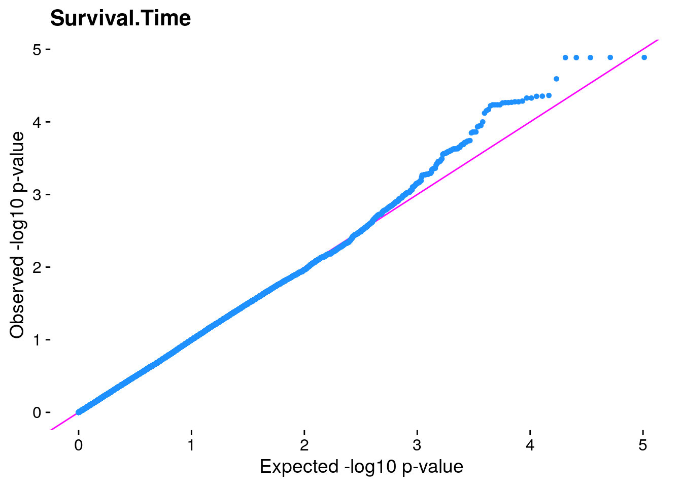
| Version | Author | Date |
|---|---|---|
| 10ccb55 | xhyuo | 2021-09-19 |
# [1] 7.891821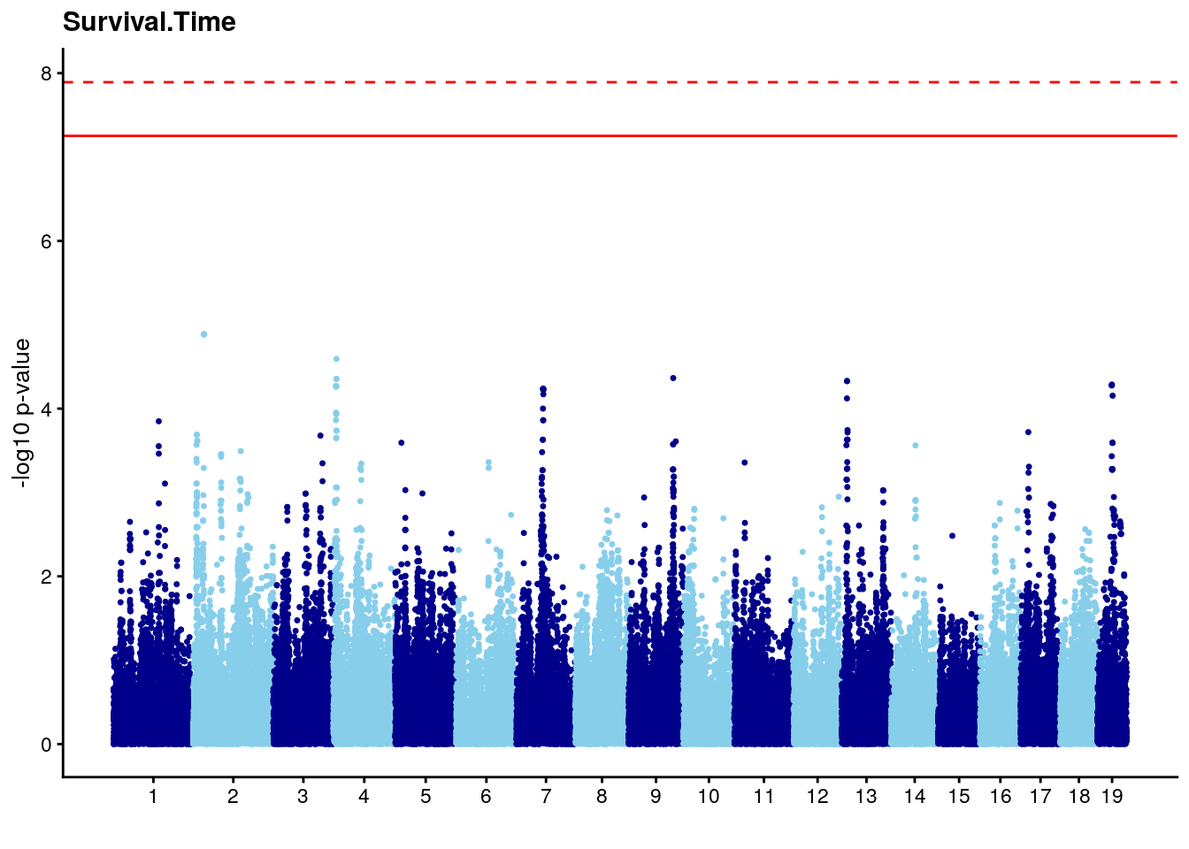
# [1] "Recovery.Time"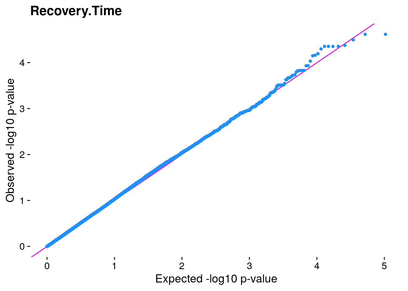
| Version | Author | Date |
|---|---|---|
| 10ccb55 | xhyuo | 2021-09-19 |
# [1] 6.628629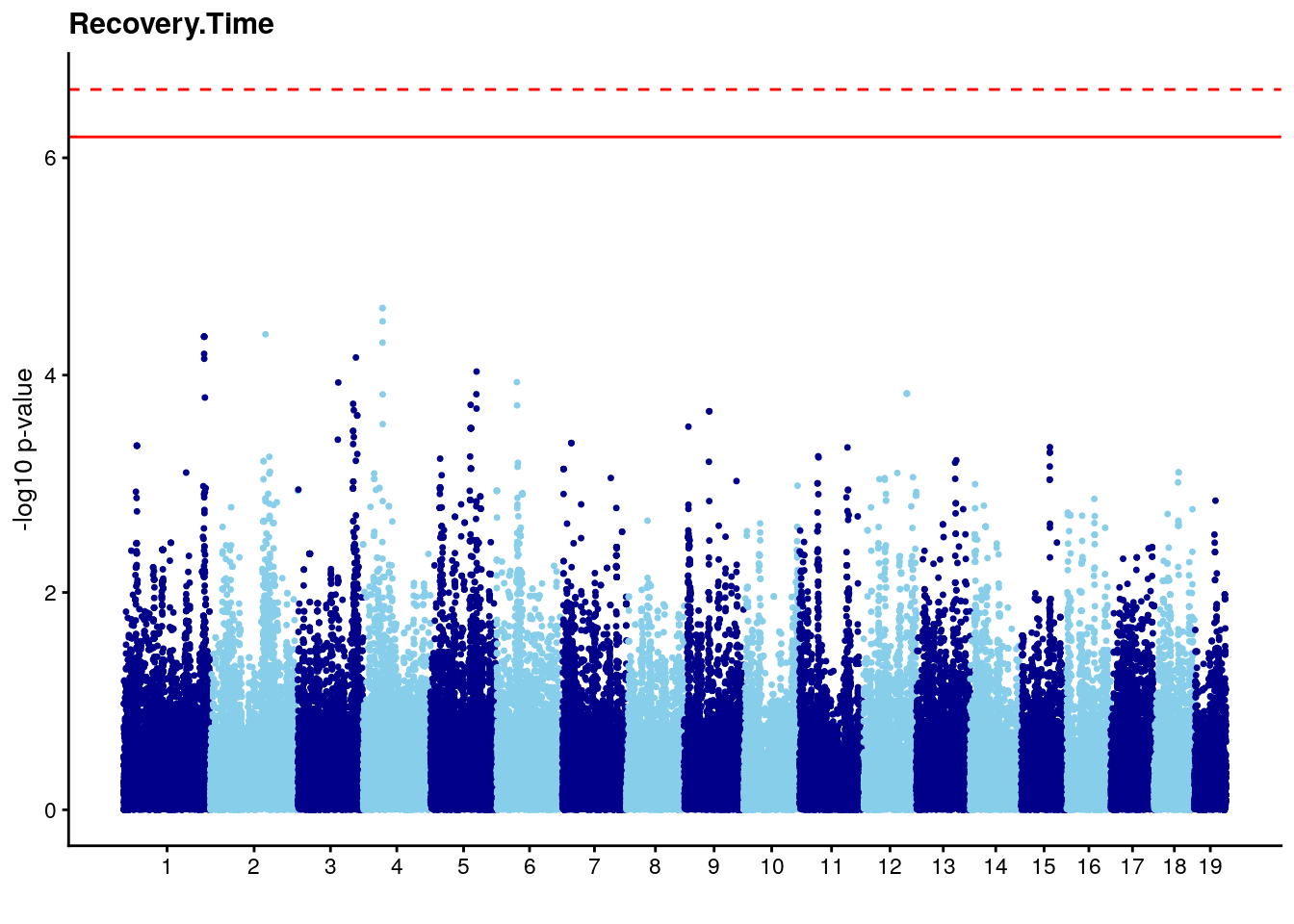
# [1] "Min.depression"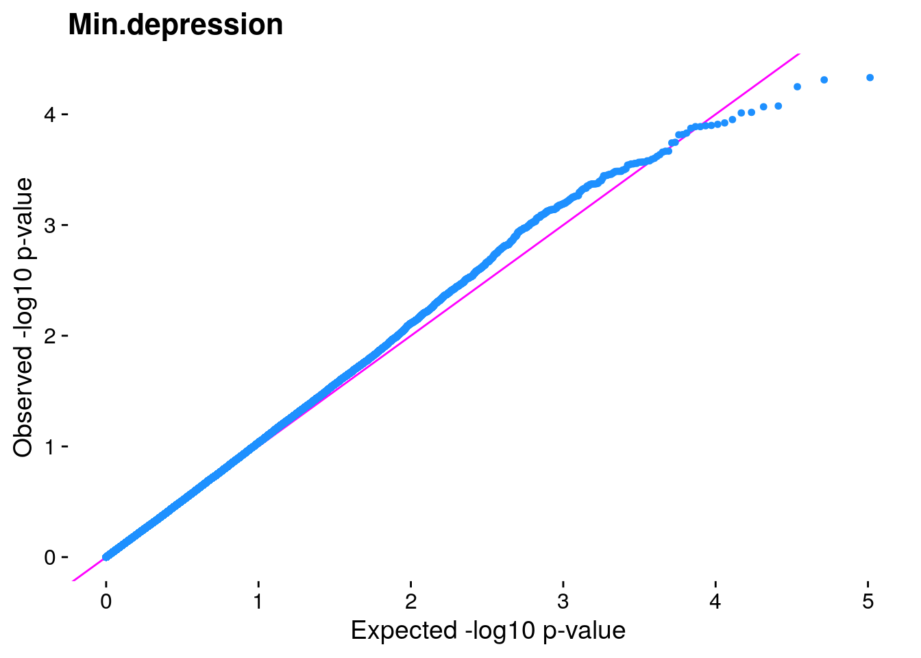
| Version | Author | Date |
|---|---|---|
| 10ccb55 | xhyuo | 2021-09-19 |
# [1] 6.092336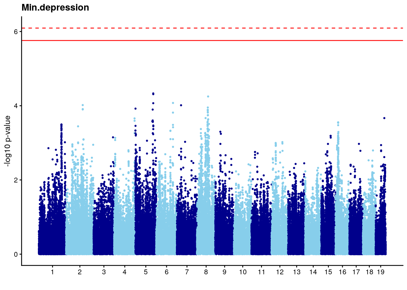
# [1] "Status_bin"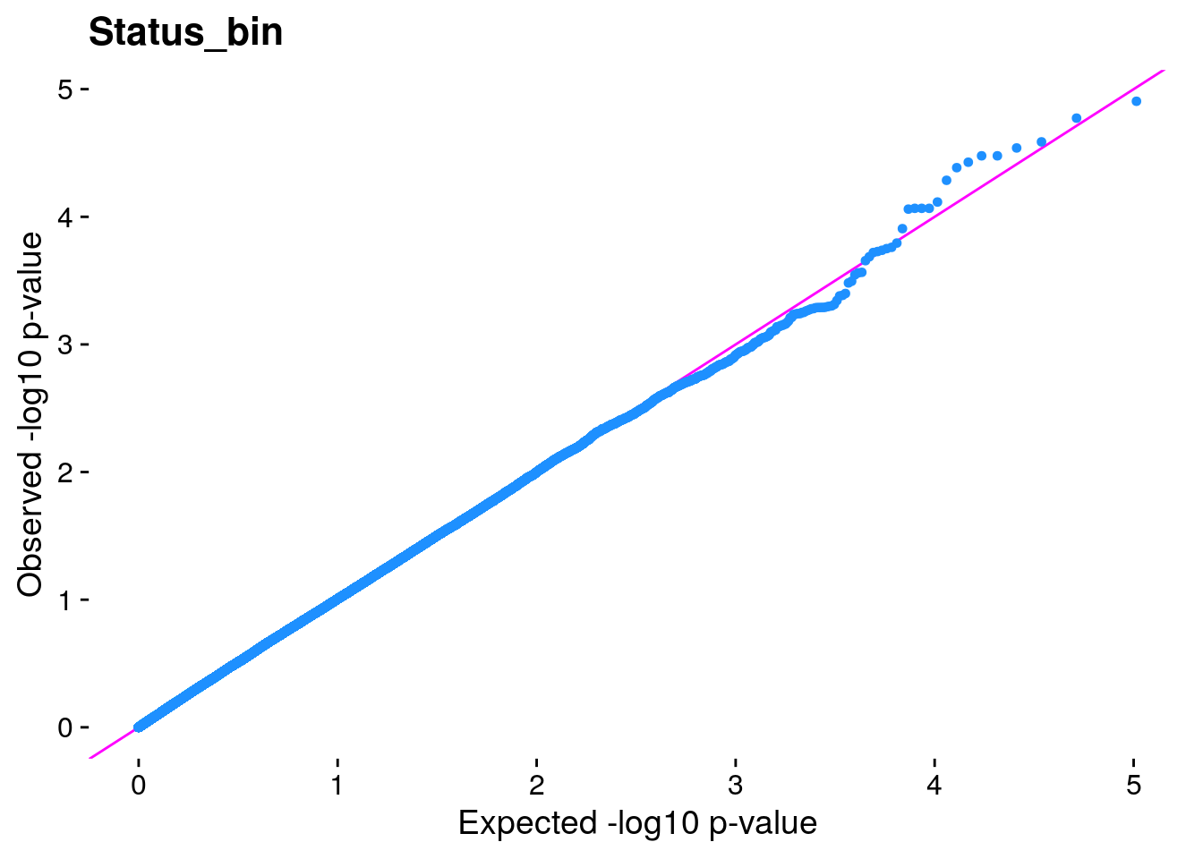
| Version | Author | Date |
|---|---|---|
| 10ccb55 | xhyuo | 2021-09-19 |
# [1] 5.854849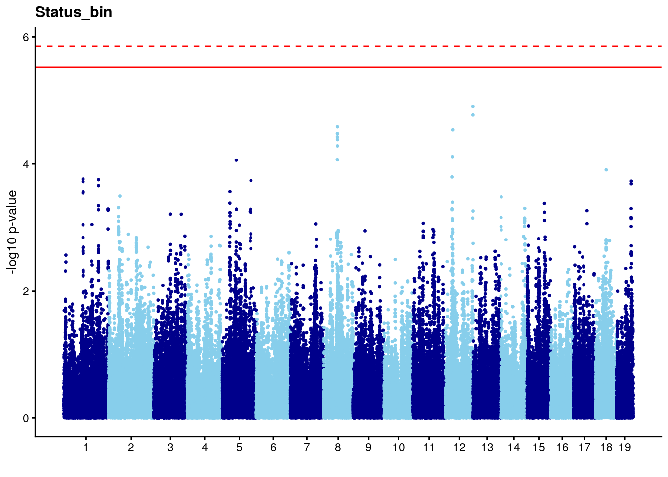
###heritability
#plot heritability by qtl2 array
load("output/Fentanyl/qtl.fentanyl.out.RData")
herit <- data.frame(Phenotype = names(unlist(qtl.morphine.hsq)),
                    Heritability = round(unlist(qtl.morphine.hsq),2))
herit <- herit %>%
  arrange(desc(Heritability))
herit$Phenotype <- factor(herit$Phenotype, levels = herit$Phenotype)
#histgram
pdf(file = paste0("data/FinalReport/GCTA/DO_Fentanyl","_heritability_by_qtl2_array.pdf"), height = 10, width = 10)
p1<-ggplot(data=herit, aes(x=Phenotype, y=Heritability)) + #, fill=Domain, color = Domain)) +
  geom_bar(stat="identity", fill = "blue", color = "blue", show.legend = FALSE) +
  scale_y_continuous(breaks=seq(0.0, 1.0, 0.1)) +
  geom_text(aes(label = Heritability, y = Heritability + 0.005), position = position_dodge(0.9),vjust = 0) +
  theme(axis.text.x = element_text(angle = 90, hjust = 1)) +
  ggtitle("Heritability by qtl2 array")
p1
dev.off()
# png
#   2
p1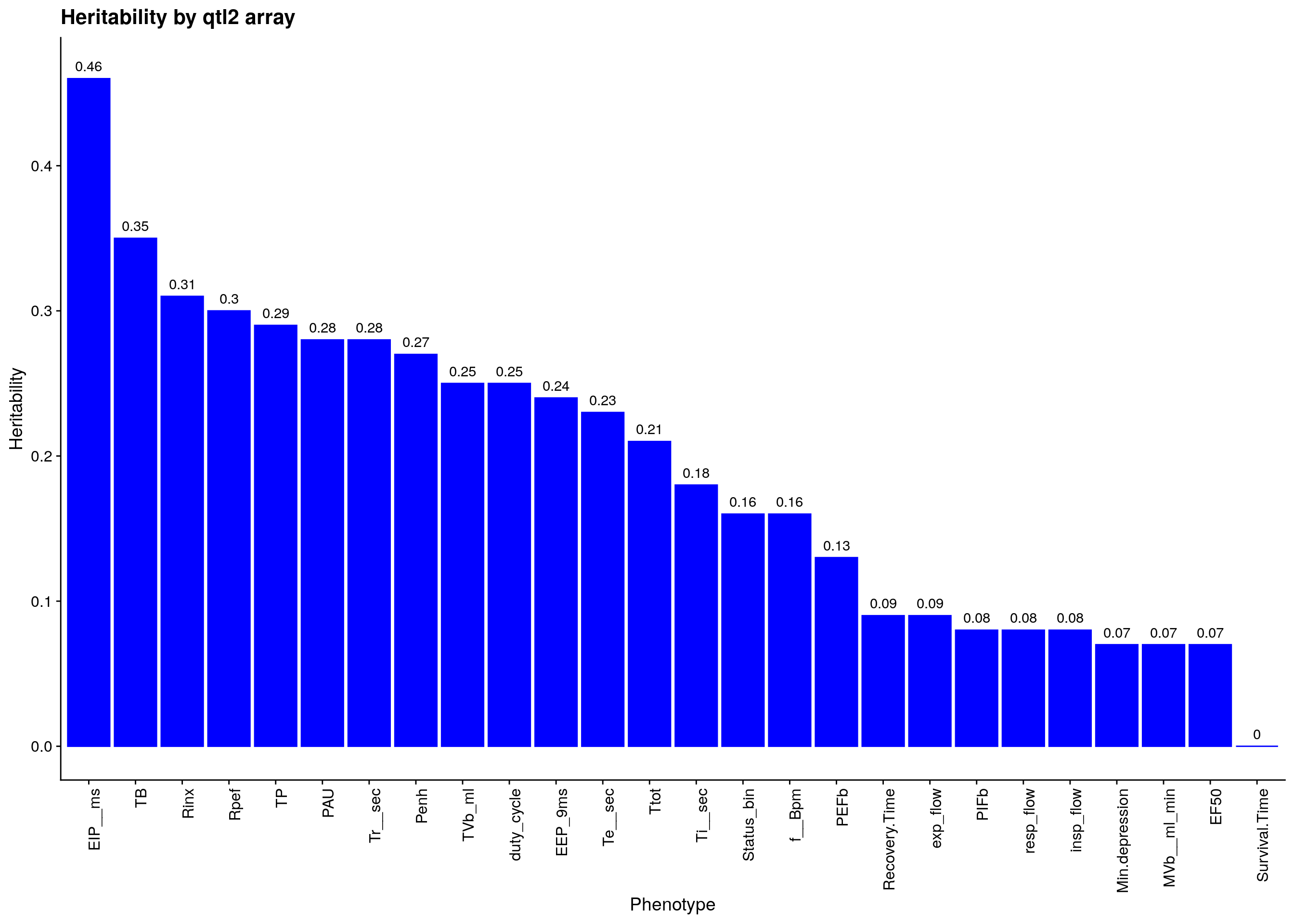
#plot heritability by qtl2 69k
load("output/Fentanyl/qtl.fentanyl.69k.out.RData")
herit <- data.frame(Phenotype = names(unlist(qtl.morphine.hsq)),
                    Heritability = round(unlist(qtl.morphine.hsq),2))
herit <- herit %>%
  arrange(desc(Heritability))
herit$Phenotype <- factor(herit$Phenotype, levels = herit$Phenotype)
#histgram
pdf(file = paste0("data/FinalReport/GCTA/DO_Fentanyl","_heritability_by_qtl2_69k.pdf"), height = 10, width = 10)
p2<-ggplot(data=herit, aes(x=Phenotype, y=Heritability)) + #, fill=Domain, color = Domain)) +
  geom_bar(stat="identity", fill = "blue", color = "blue", show.legend = FALSE) +
  scale_y_continuous(breaks=seq(0.0, 1.0, 0.1)) +
  geom_text(aes(label = Heritability, y = Heritability + 0.005), position = position_dodge(0.9),vjust = 0) +
  theme(axis.text.x = element_text(angle = 90, hjust = 1)) +
  ggtitle("Heritability by qtl2 69k")
p2
dev.off()
# png
#   2
p2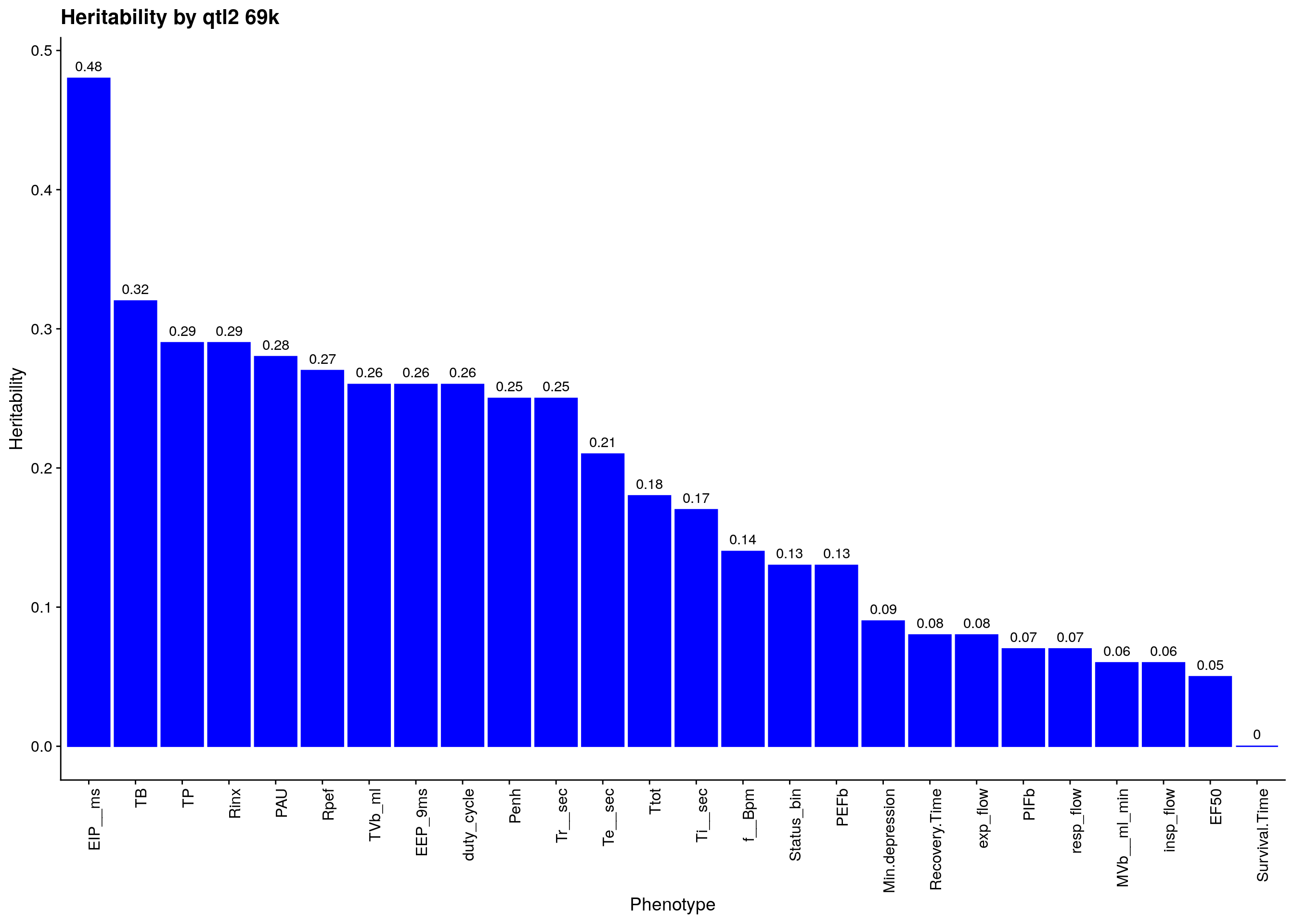
#plot heritability by GCTA
h <- read.csv("data/FinalReport/GCTA/DO_Fentanyl_heritability_by_GCTA.csv", header = TRUE)
h <- h %>%
  arrange(desc(Heritability))
h$Phenotype <- factor(h$Phenotype, levels = h$Phenotype)
h$Heritability <- round(h$Heritability,2)
#histgram
pdf(file = paste0("data/FinalReport/GCTA/DO_Fentanyl","_heritability_by_GCTA.pdf"), height = 10, width = 10)
p3<-ggplot(data=h, aes(x=Phenotype, y=Heritability)) + #, fill=Domain, color = Domain)) +
  geom_bar(stat="identity", fill = "blue", color = "blue", show.legend = FALSE) +
  scale_y_continuous(breaks=seq(0.0, 1.0, 0.1)) +
  geom_text(aes(label = Heritability, y = Heritability + 0.005), position = position_dodge(0.9),vjust = 0) +
  theme(axis.text.x = element_text(angle = 90, hjust = 1)) +
  ggtitle("Heritability by GCTA")
p3
dev.off()
# png
#   2
p3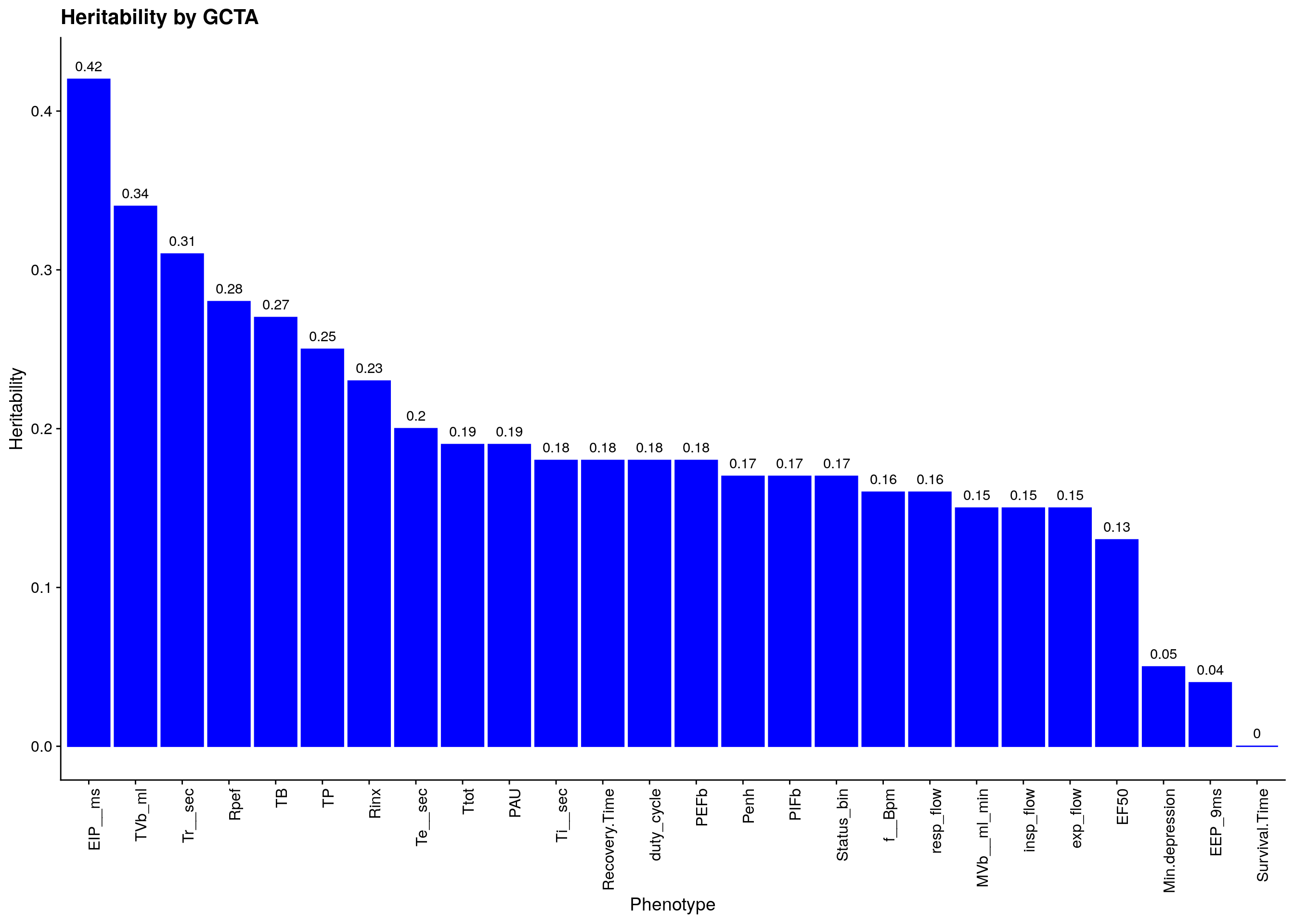
Plot qtl mapping on array male
load("output/Fentanyl/qtl.fentanyl.out.male.RData")

#genome-wide plot
for(i in names(qtl.morphine.out)){
  par(mar=c(5.1, 4.1, 1.1, 1.1))
  ymx <- maxlod(qtl.morphine.out[[i]]) # overall maximum LOD score
  plot(qtl.morphine.out[[i]], map=gm$pmap, lodcolumn=1, col="slateblue", ylim=c(0, max(sapply(qtl.morphine.out, maxlod)) +2))
  abline(h=summary(qtl.morphine.operm[[i]], alpha=c(0.10, 0.05, 0.01))[[1]], col="red")
  abline(h=summary(qtl.morphine.operm[[i]], alpha=c(0.10, 0.05, 0.01))[[2]], col="red")
  abline(h=summary(qtl.morphine.operm[[i]], alpha=c(0.10, 0.05, 0.01))[[3]], col="red")
  title(main = paste0("DO_fentanyl_",i))
}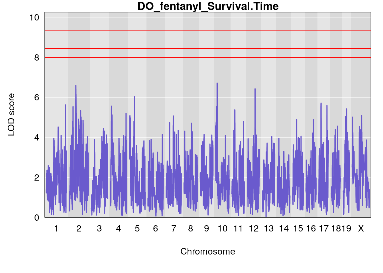
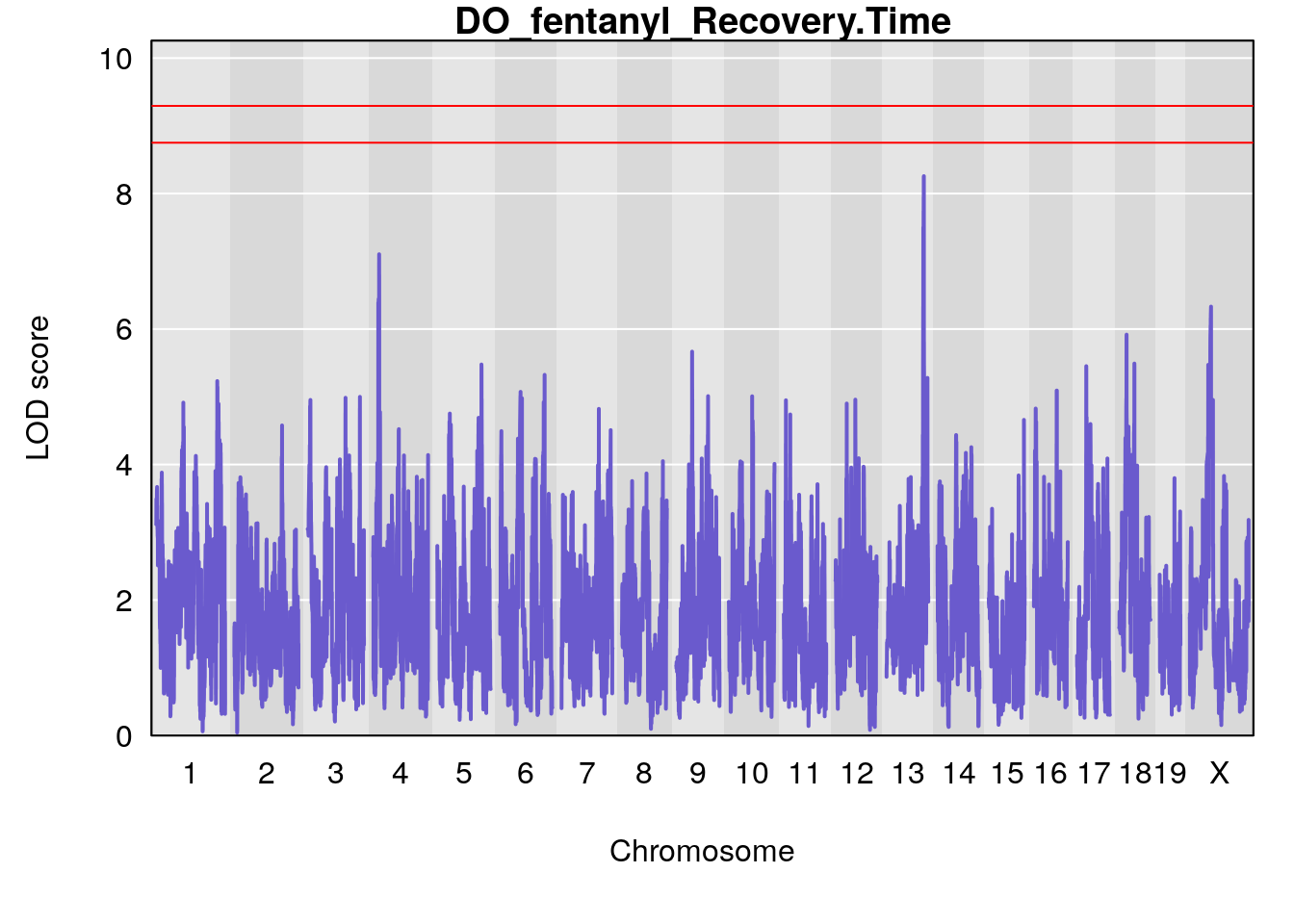
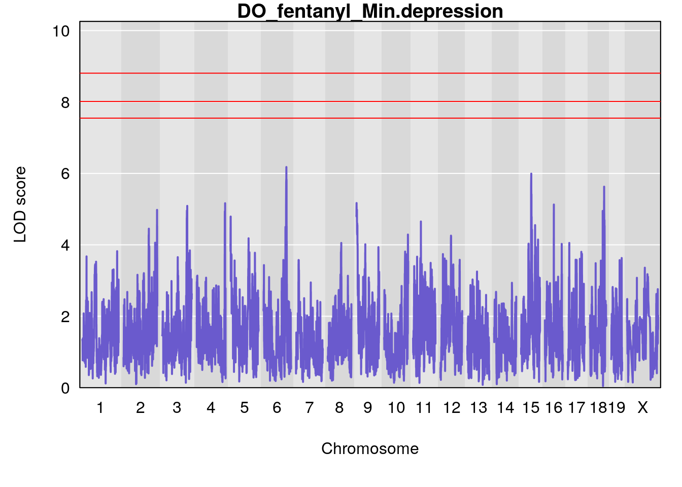
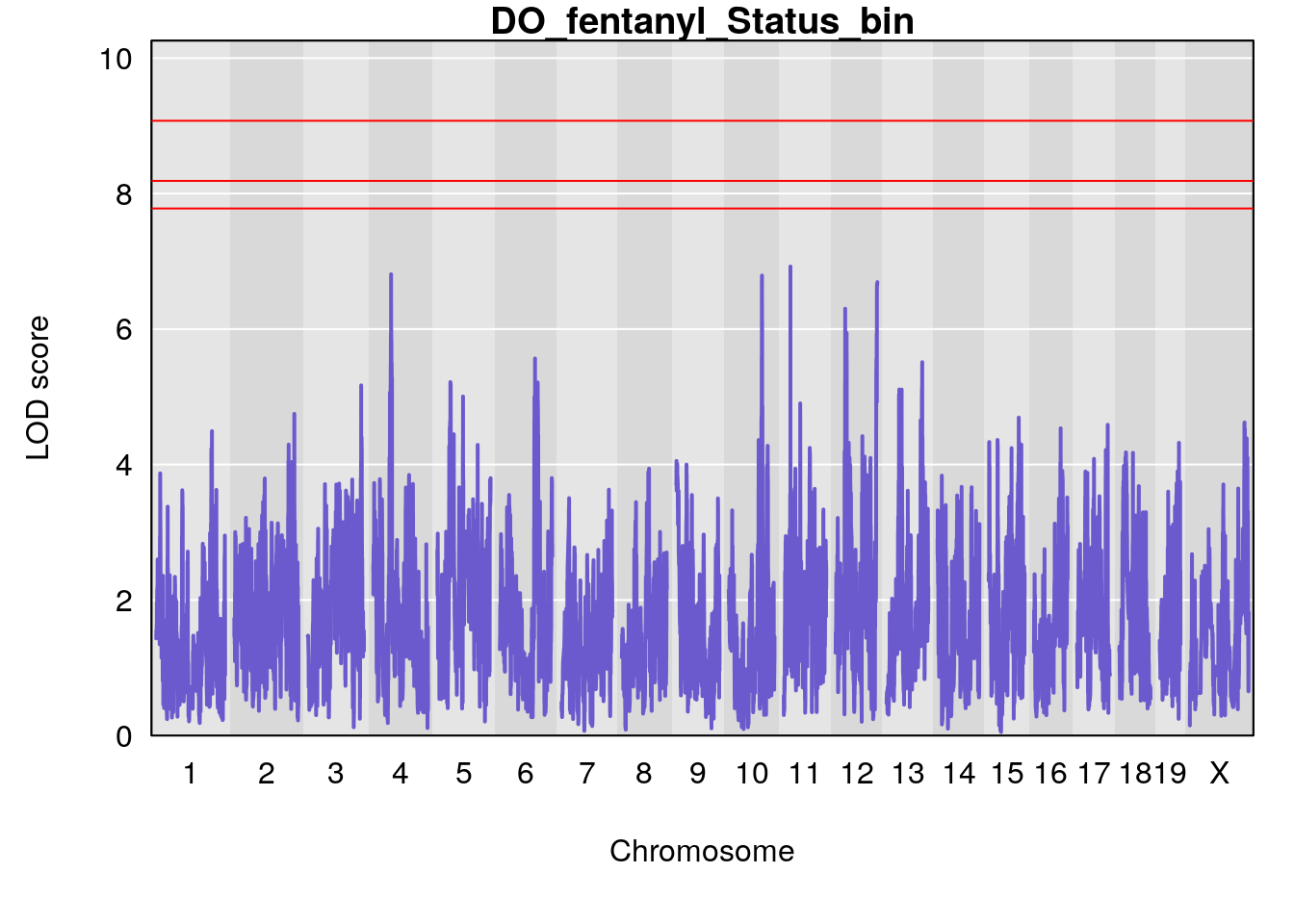
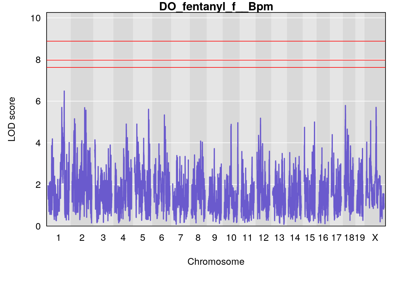
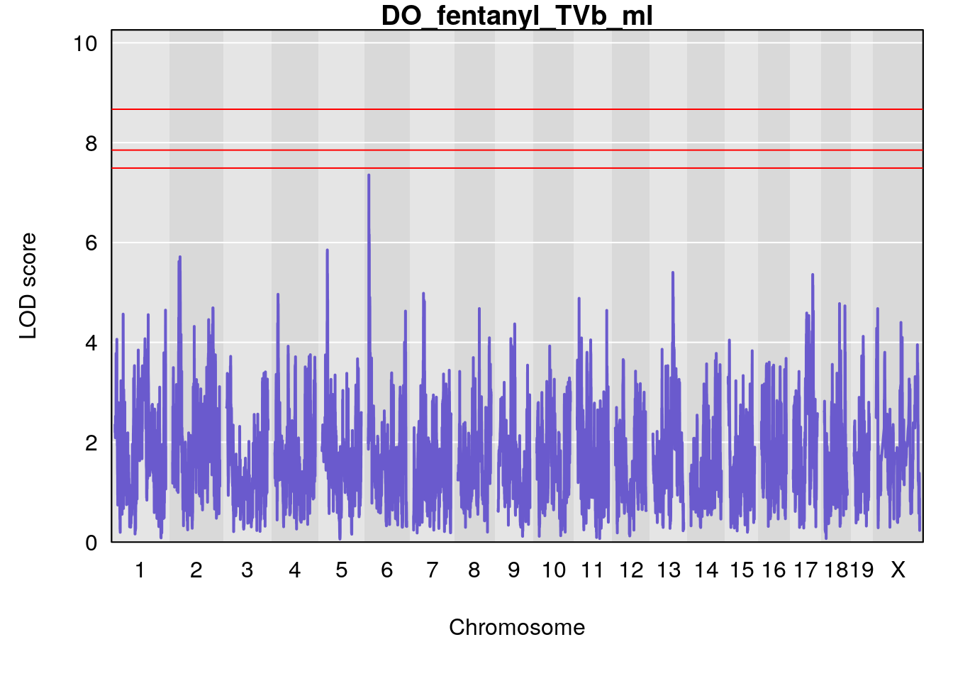
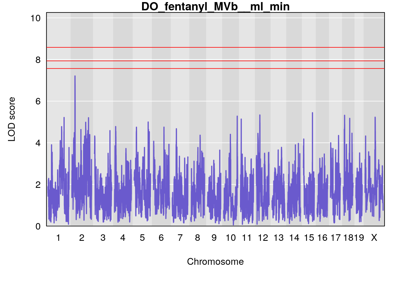
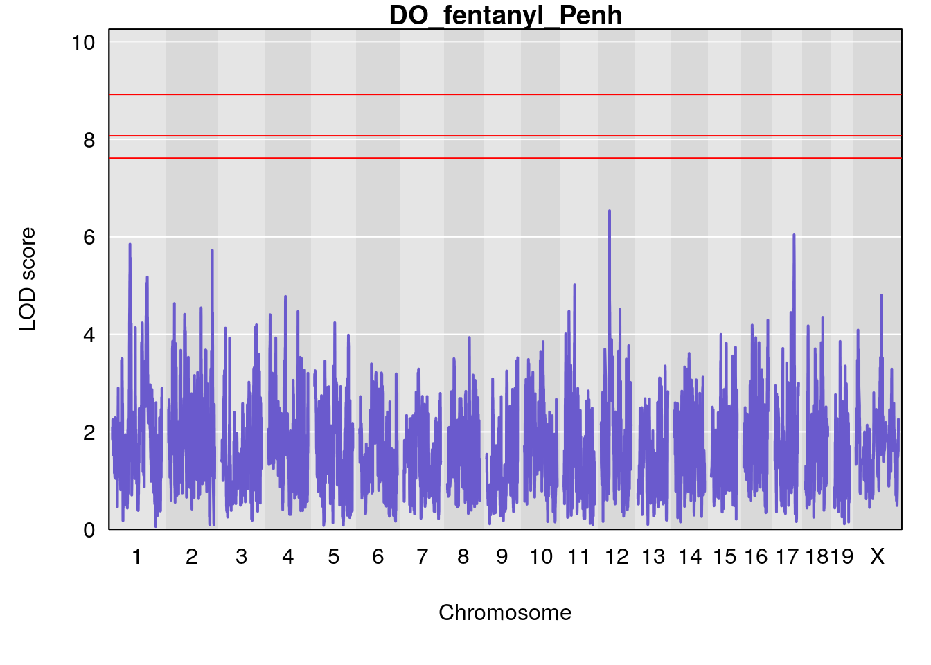

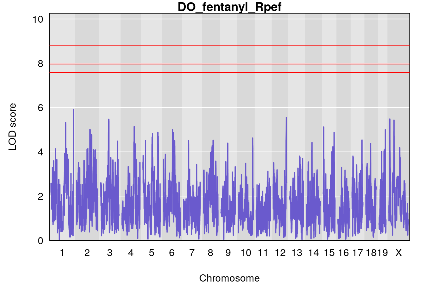
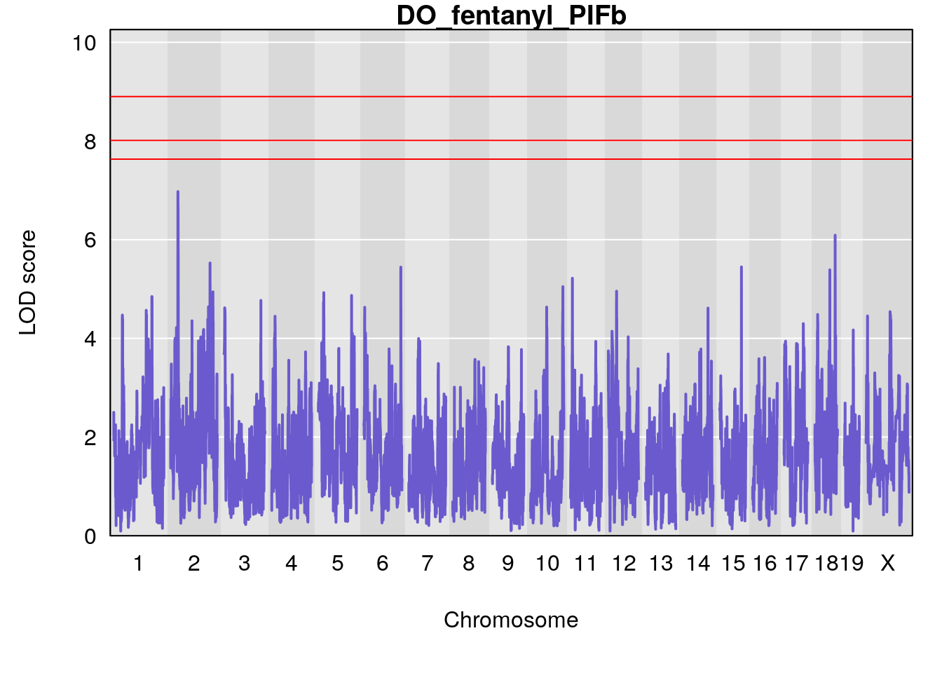

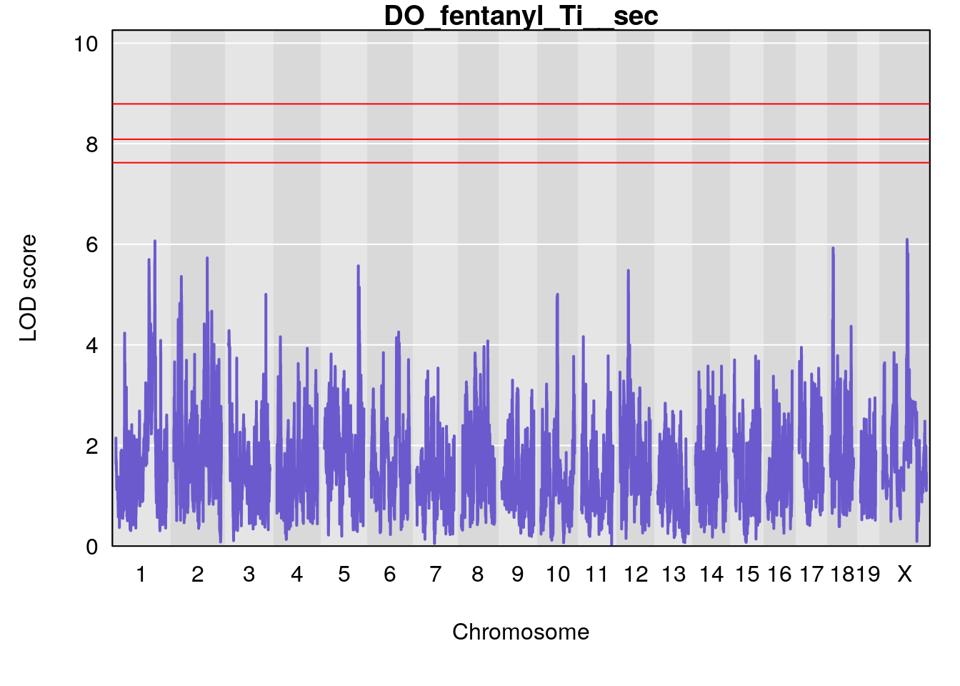
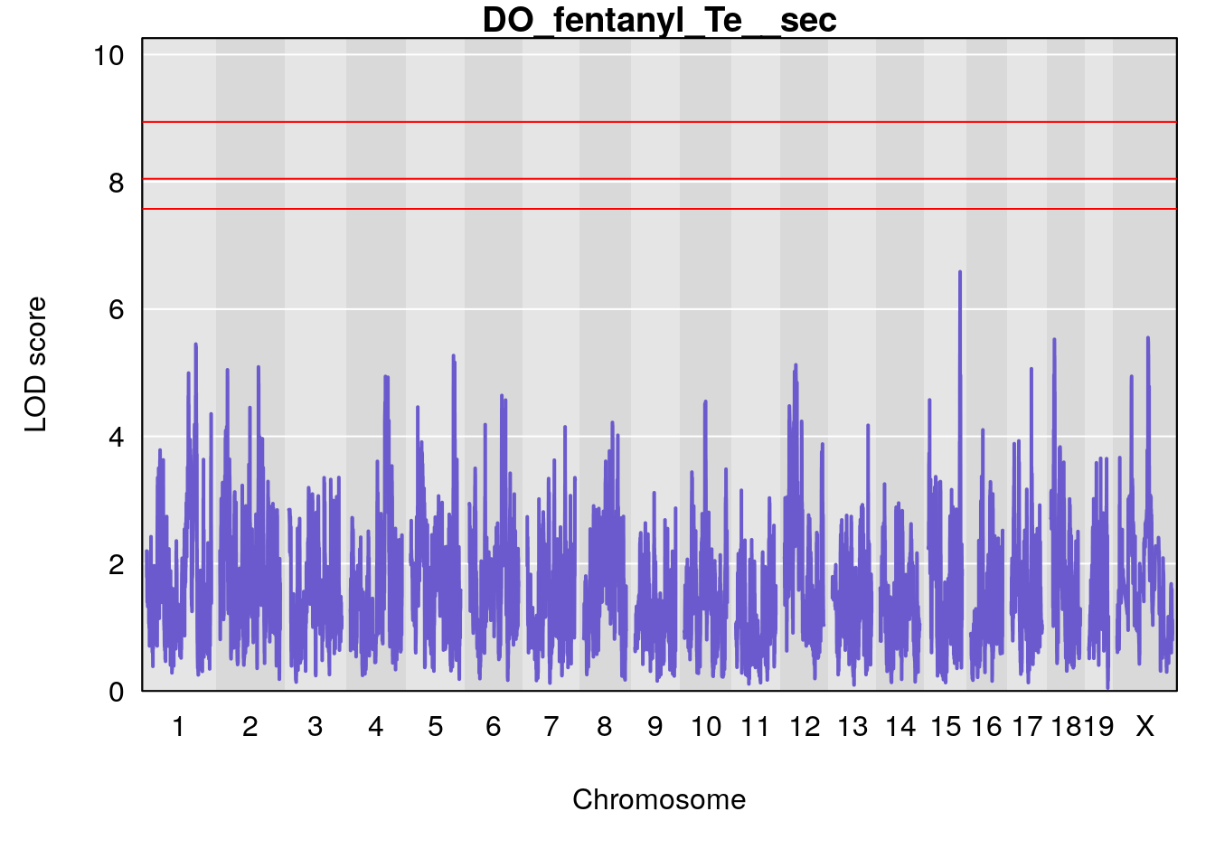
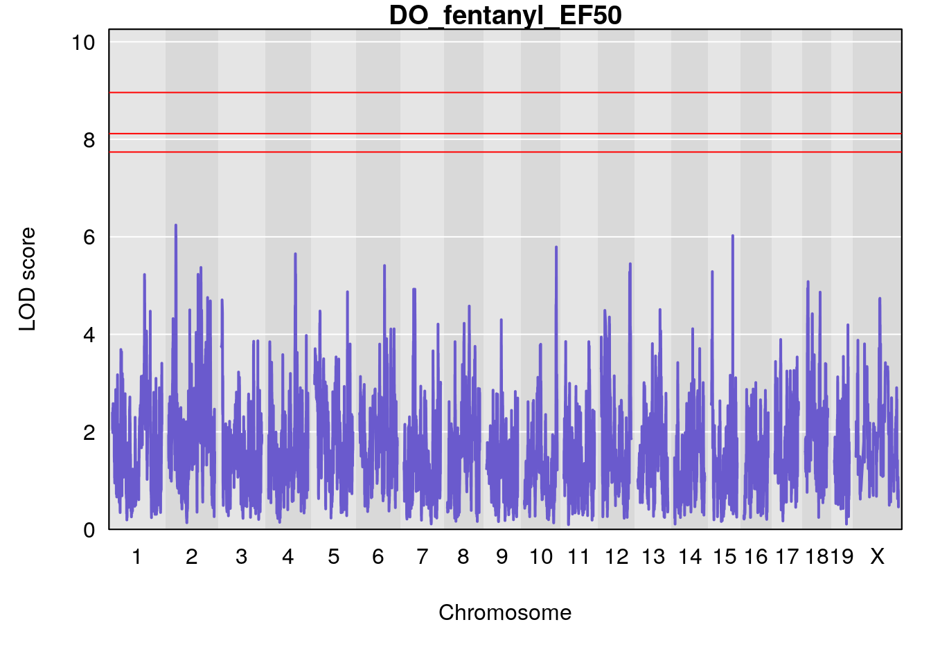
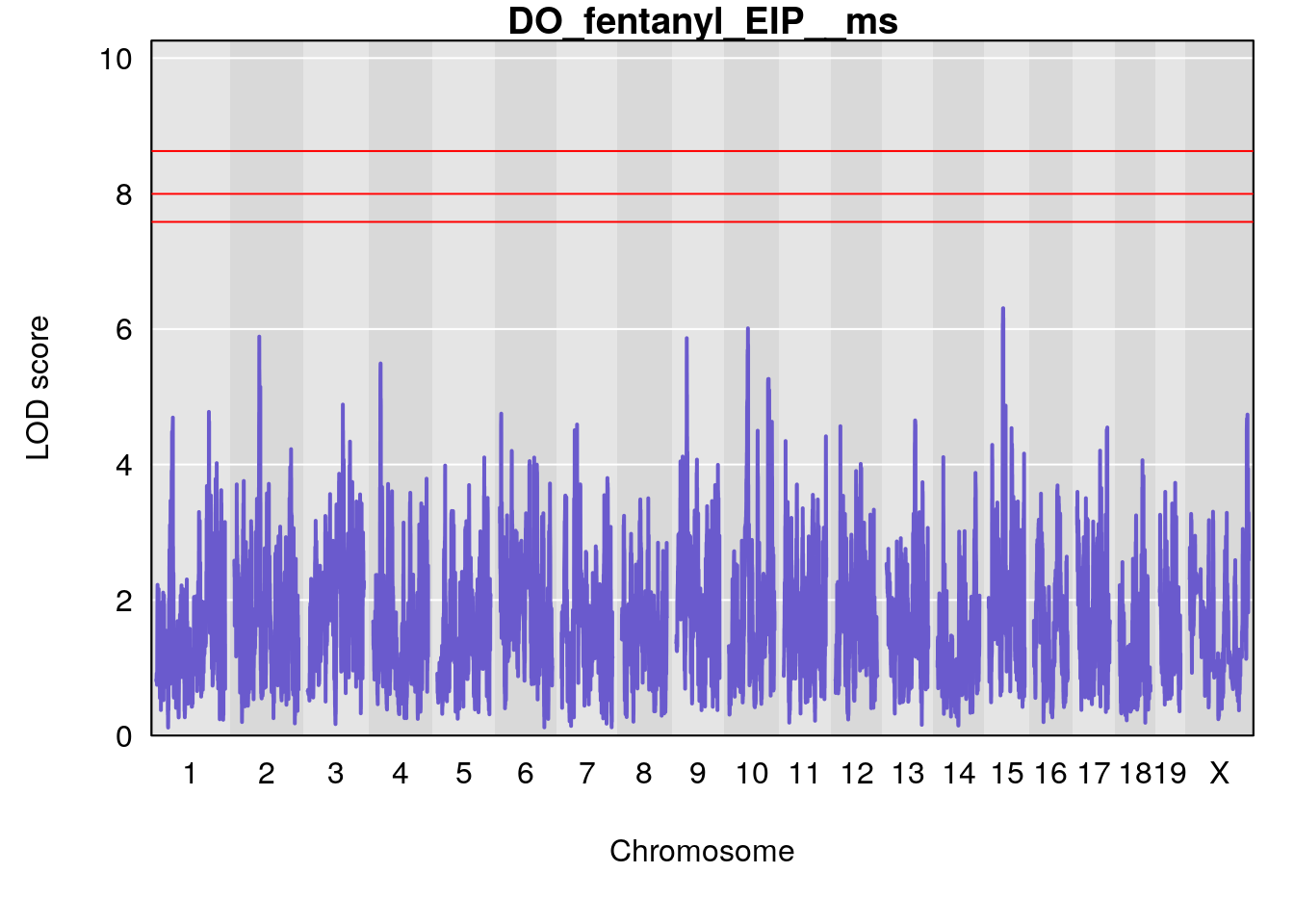
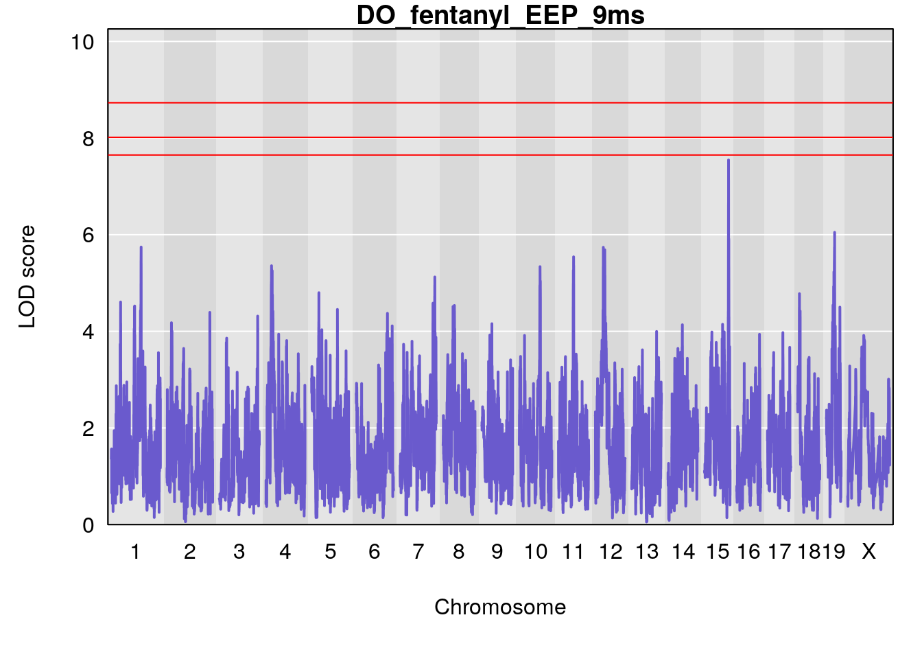
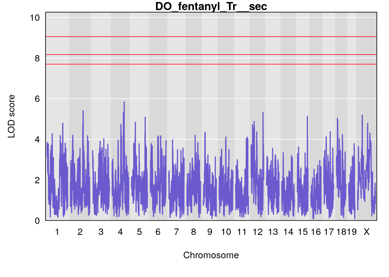
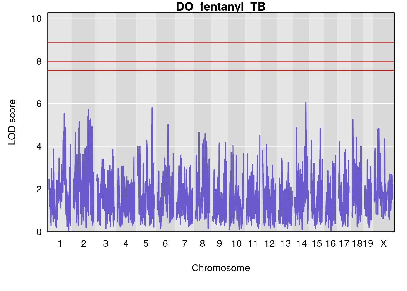
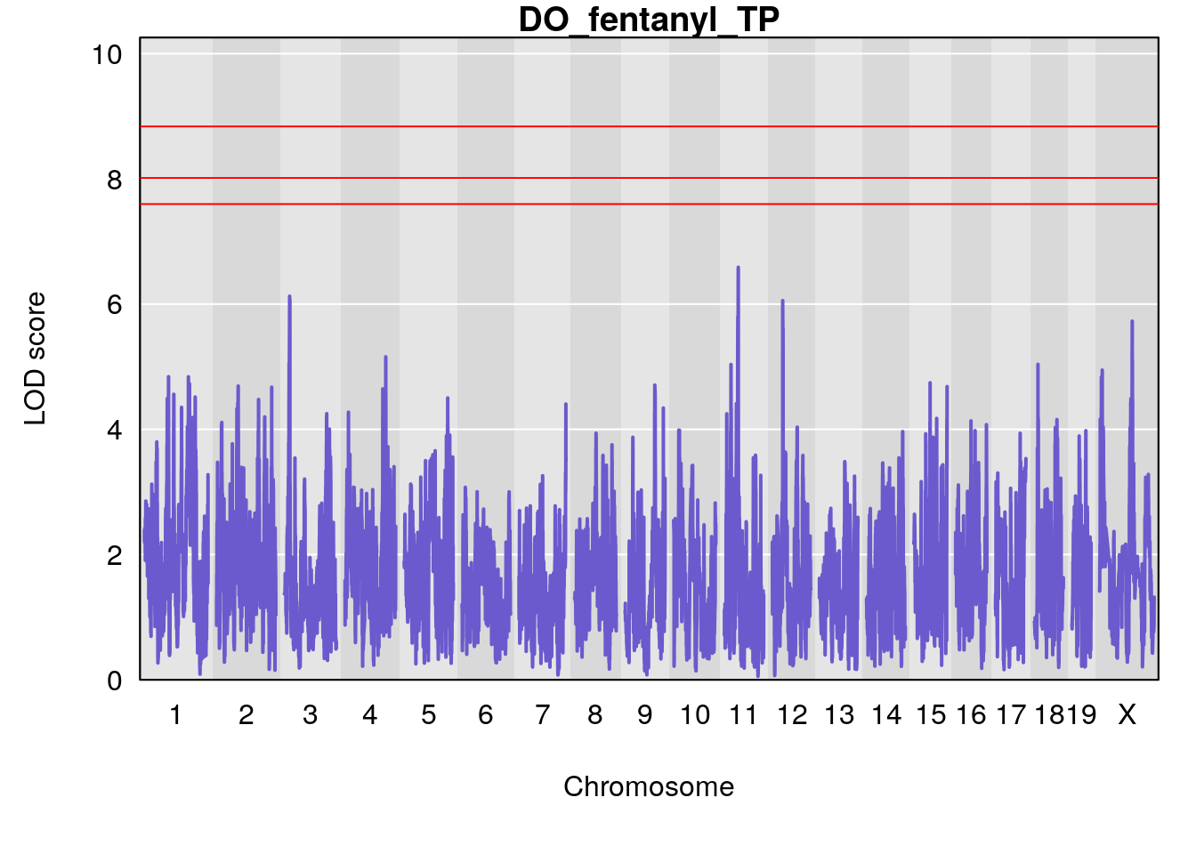
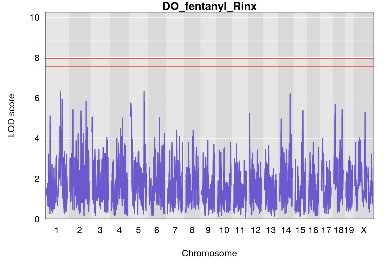
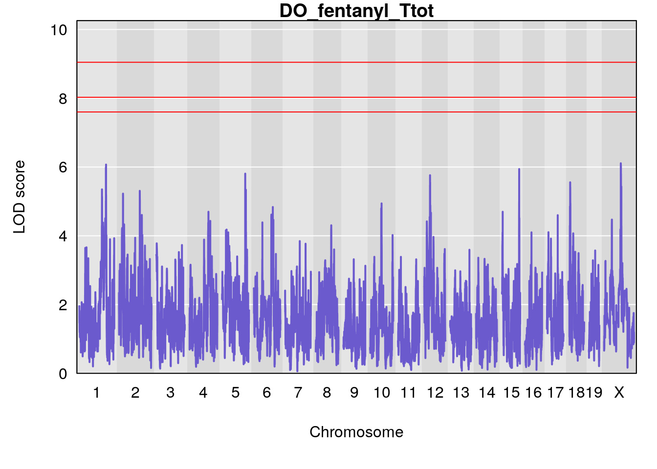

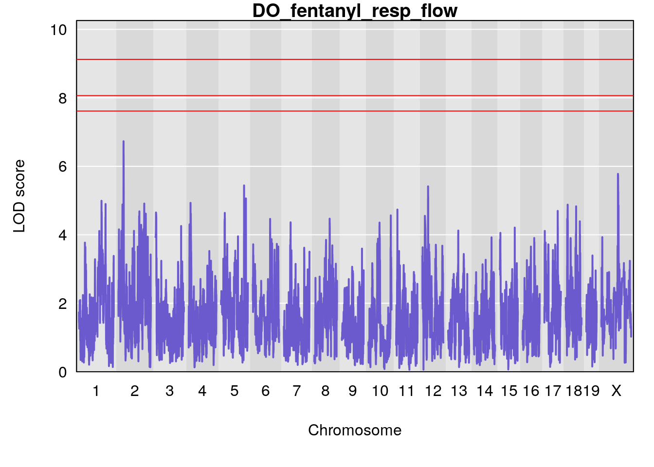
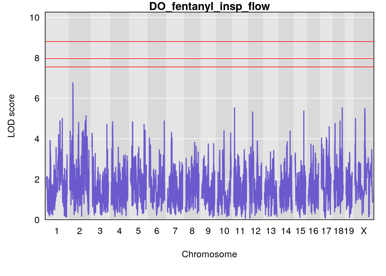
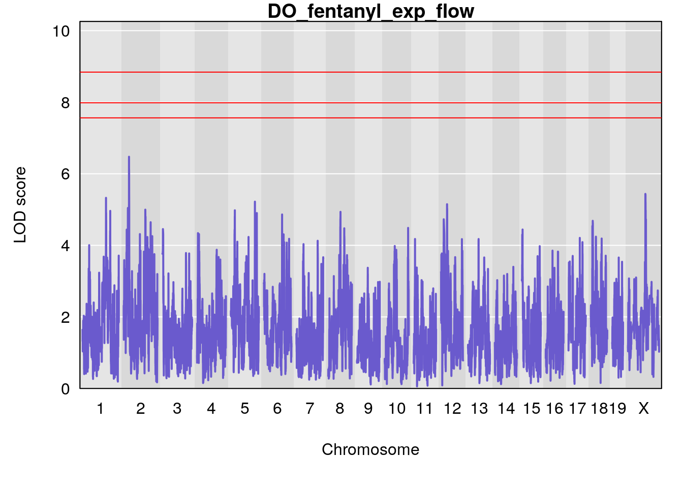
#peaks coeff plot
for(i in names(qtl.morphine.out)){
  print(i)
  peaks <- find_peaks(qtl.morphine.out[[i]], map=gm$pmap, threshold=6, drop=1.5)
  print(peaks)
  if(dim(peaks)[1] != 0){
    for(p in 1:dim(peaks)[1]) {
      print(p)
      chr <-peaks[p,3]
      #coeff plot
      par(mar=c(4.1, 4.1, 0.6, 0.6))
      plot_coefCC(coef_c1[[i]][[p]], gm$pmap[chr], scan1_output=qtl.morphine.out[[i]], bgcolor="gray95", legend=NULL)
      plot_coefCC(coef_c2[[i]][[p]], gm$pmap[chr], scan1_output=qtl.morphine.out[[i]], bgcolor="gray95", legend=NULL)
      plot(out_snps[[i]][[p]]$lod, out_snps[[i]][[p]]$snpinfo, drop_hilit=1.5, genes=out_genes[[i]][[p]])
    }
  }
}
# [1] "Survival.Time"
#   lodindex lodcolumn chr      pos      lod     ci_lo     ci_hi
# 1        1    pheno1   2 64.51902 6.583905 37.814828 109.92657
# 2        1    pheno1   5 49.81026 6.033204  7.160707  50.93606
# 3        1    pheno1  10 16.47363 6.706261 13.882119  18.21415
# 4        1    pheno1  12 76.37279 6.419734 76.349906  77.00267
# [1] 1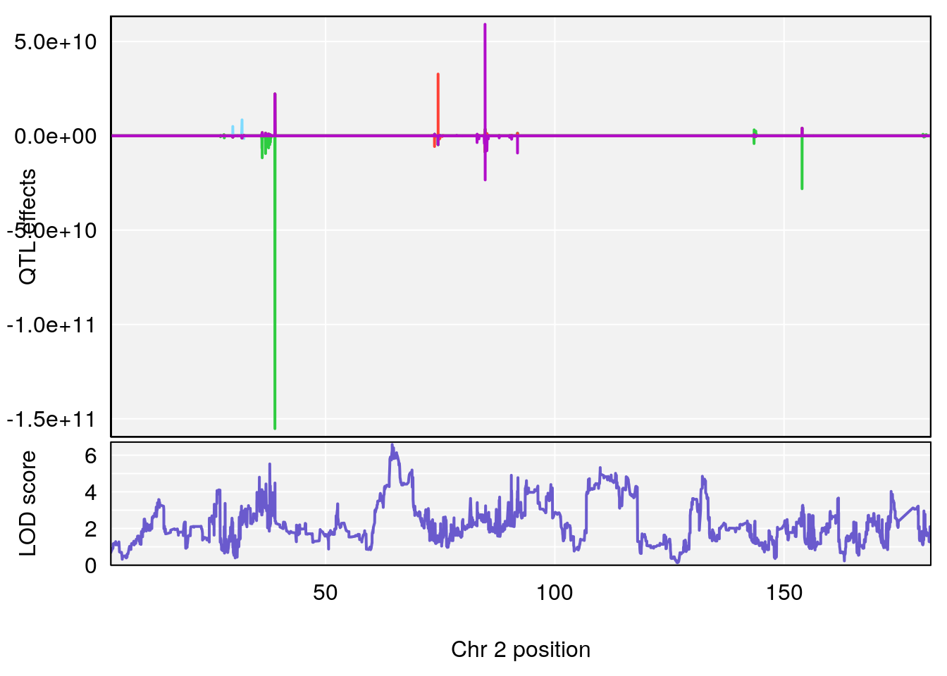
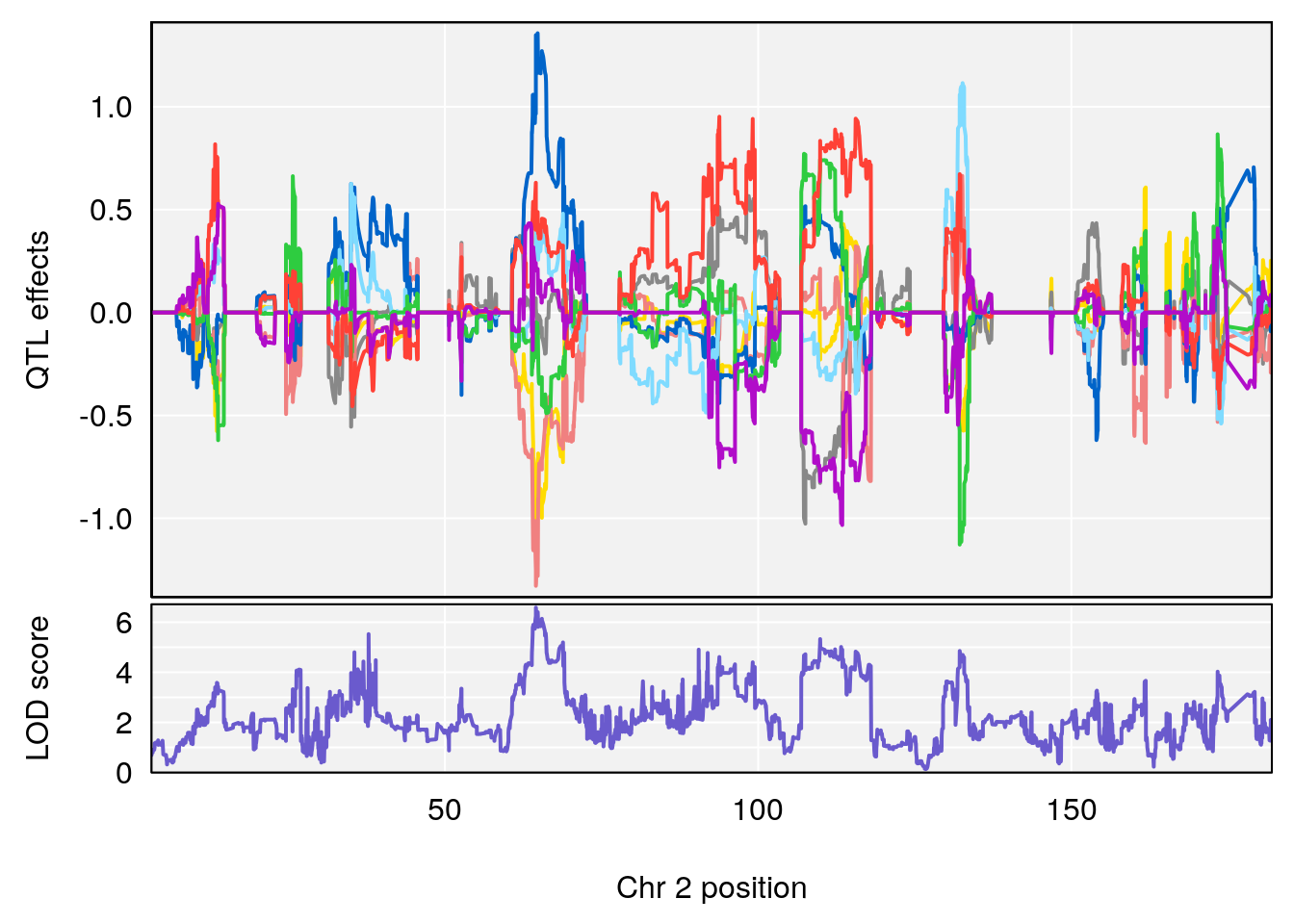
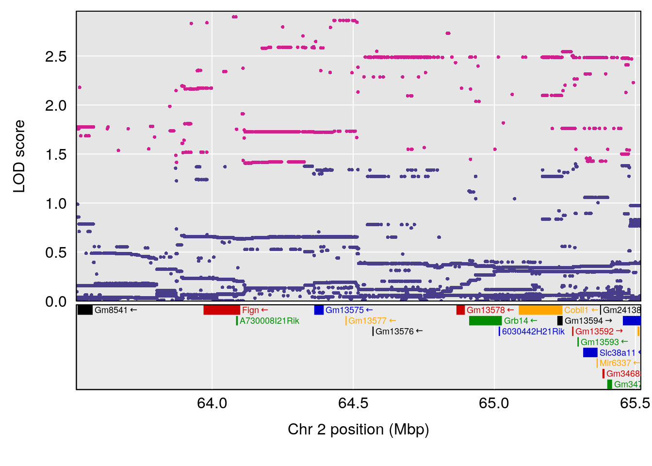
# [1] 2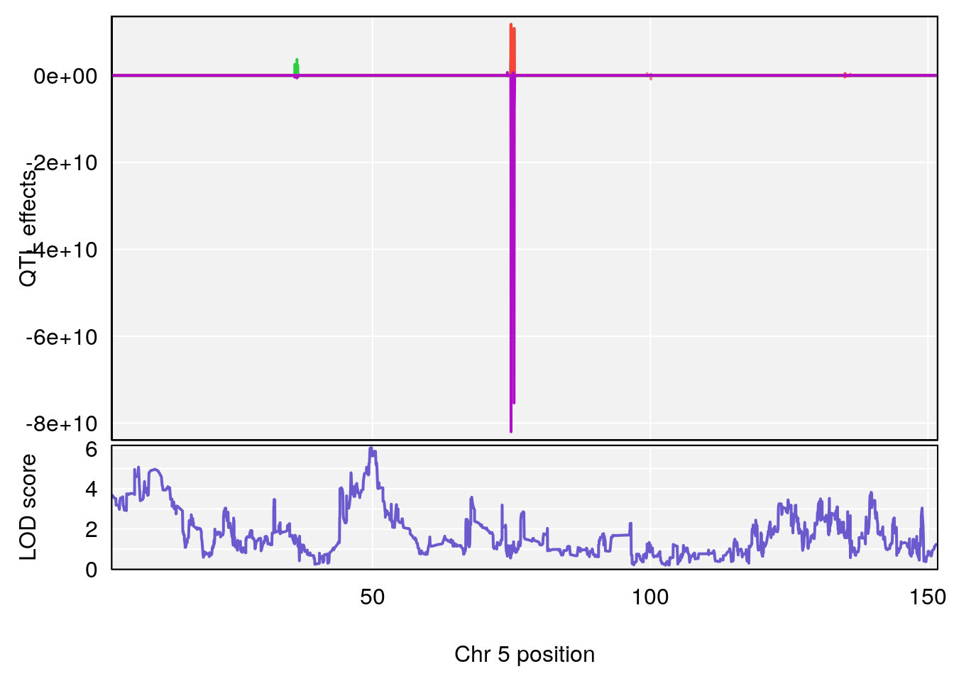
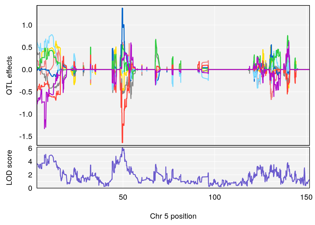
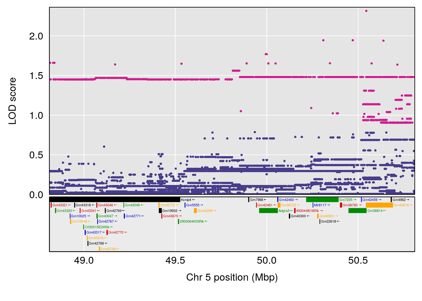
# [1] 3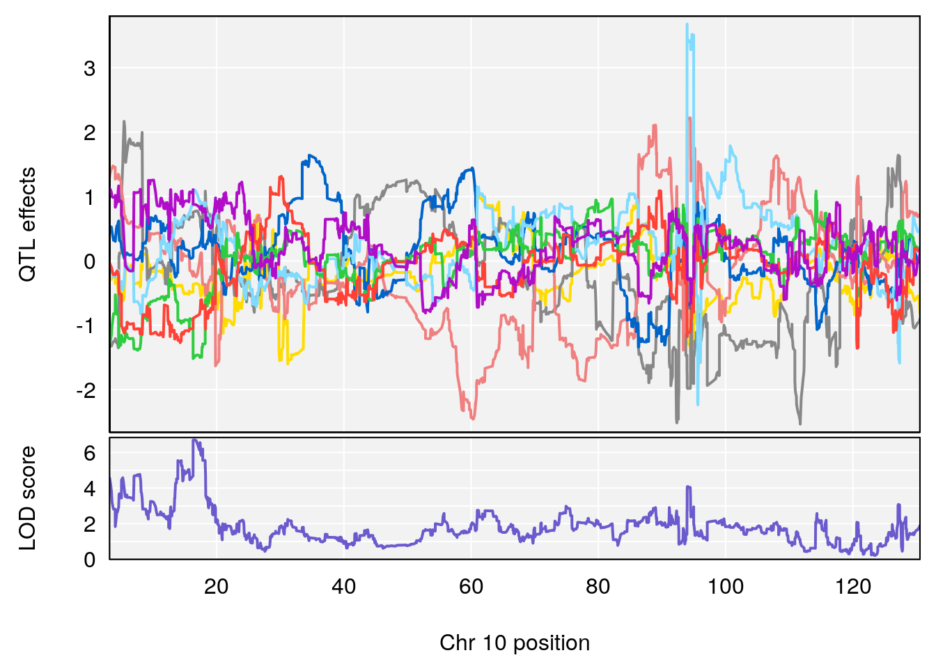
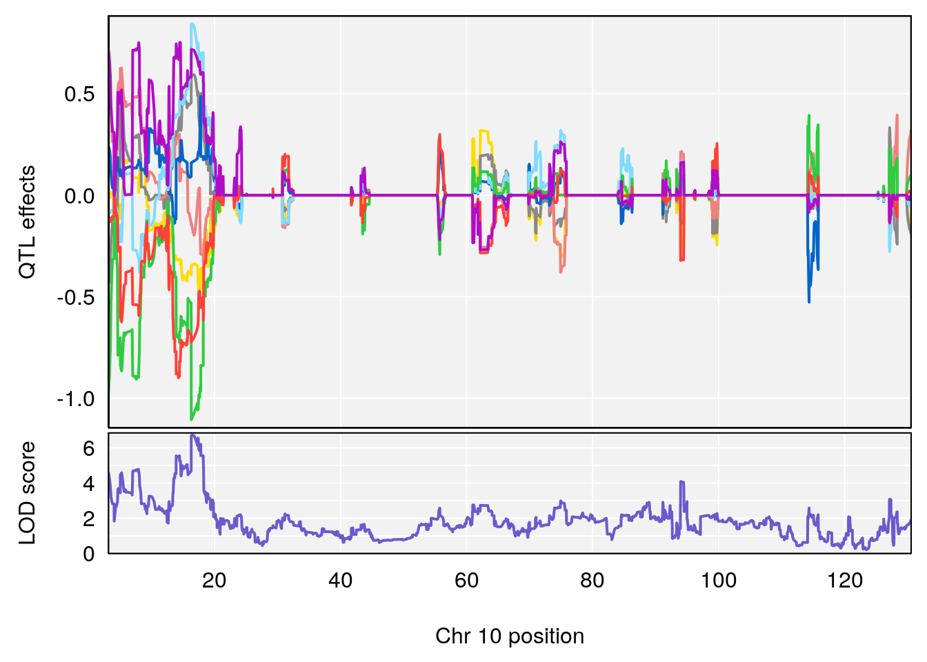
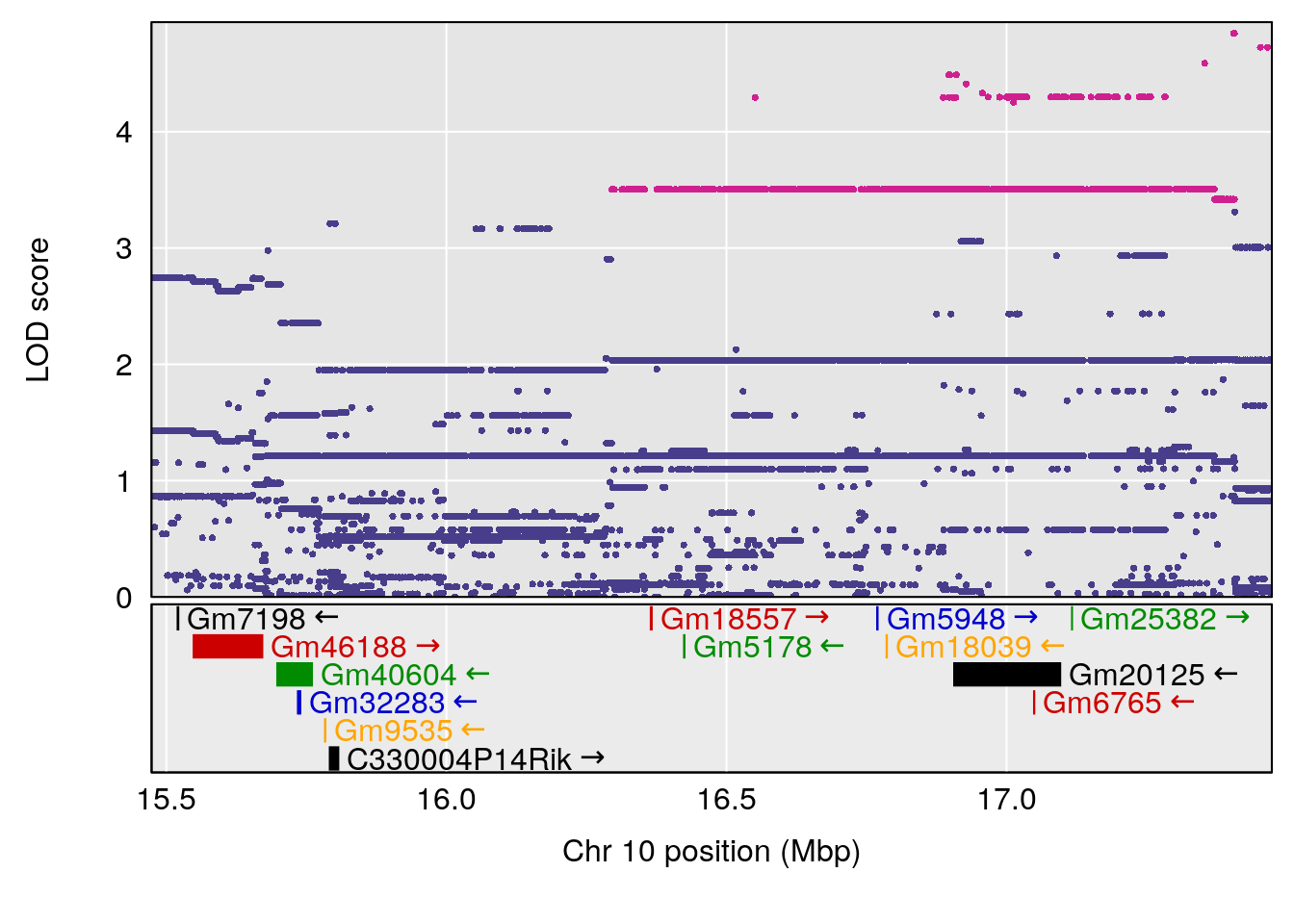
# [1] 4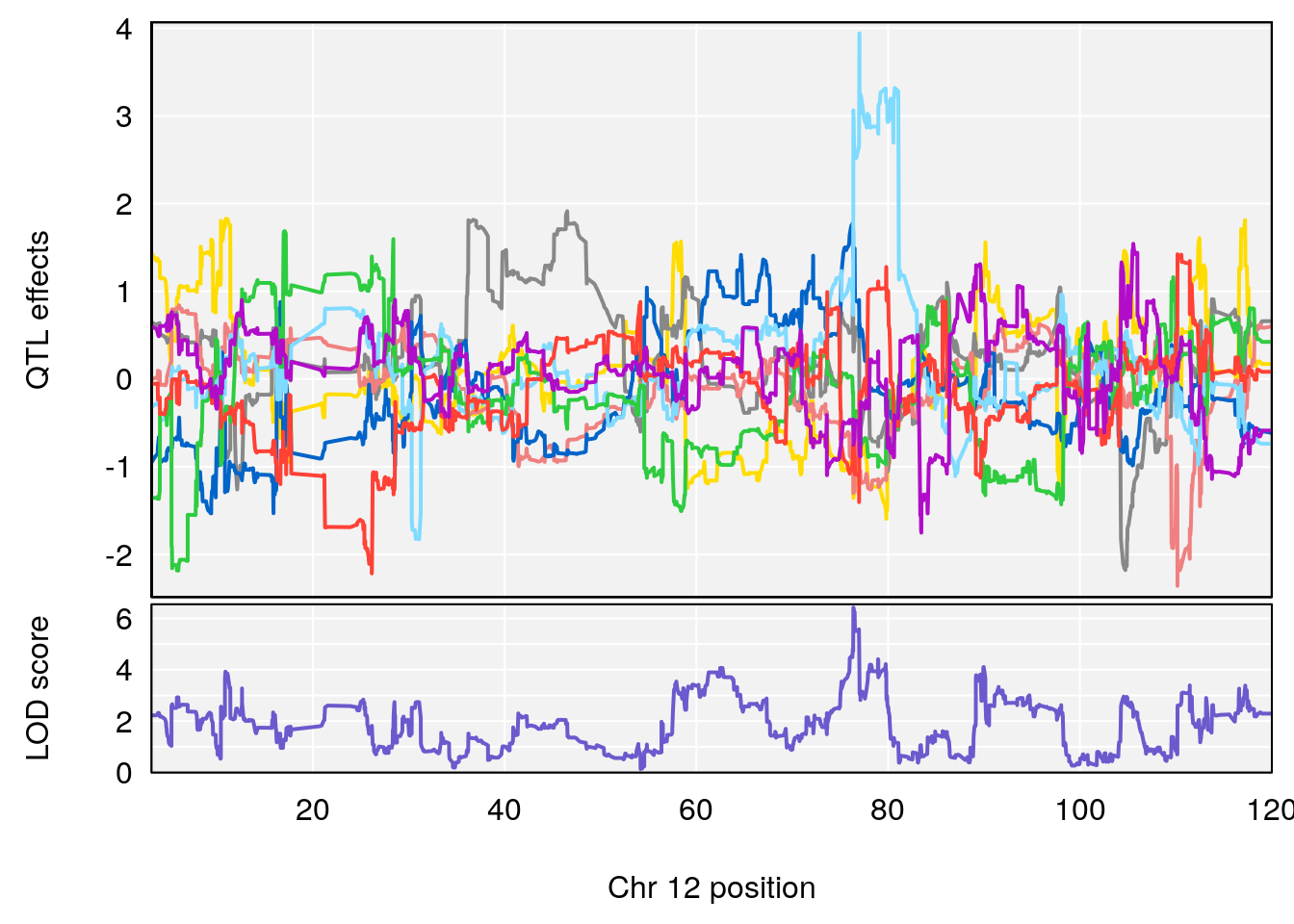
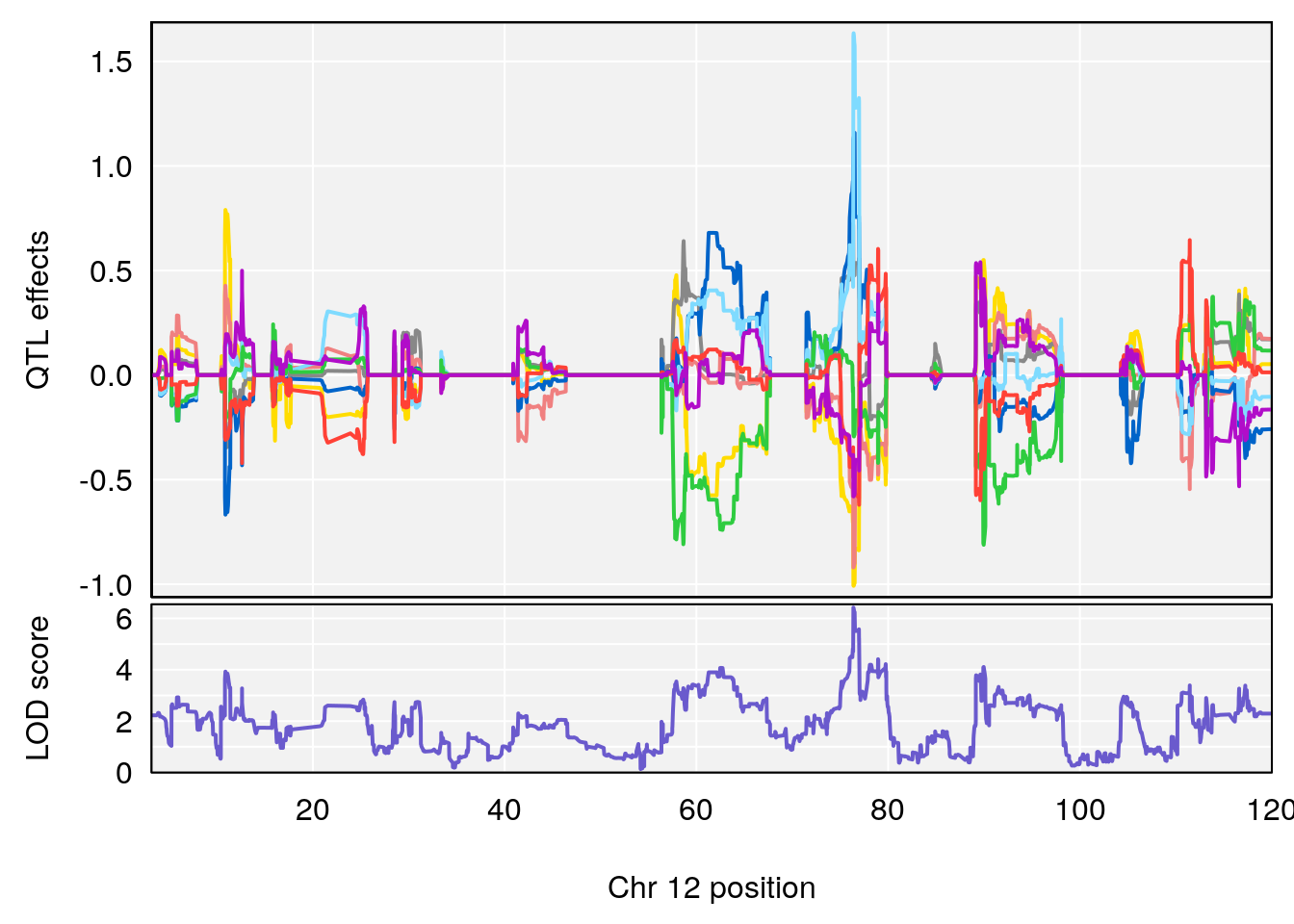
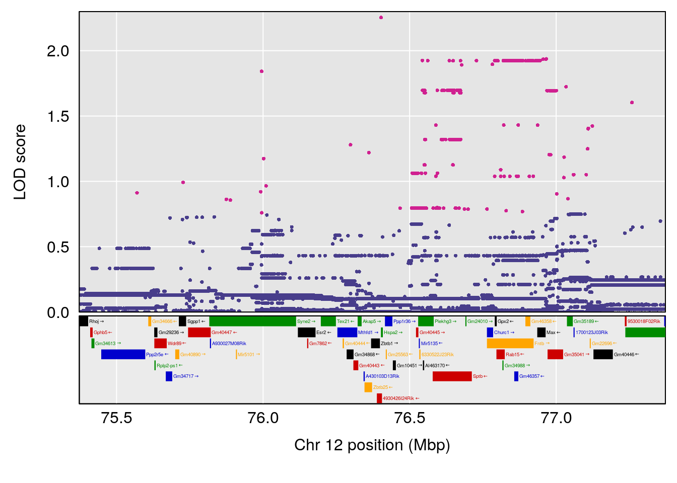
# [1] "Recovery.Time"
#   lodindex lodcolumn chr       pos      lod     ci_lo     ci_hi
# 1        1    pheno1   4  19.83766 7.103874  17.27852  20.15051
# 2        1    pheno1  13 107.08925 8.256899 105.30604 107.21017
# 3        1    pheno1   X  64.95178 6.331099  57.02997  70.45663
# [1] 1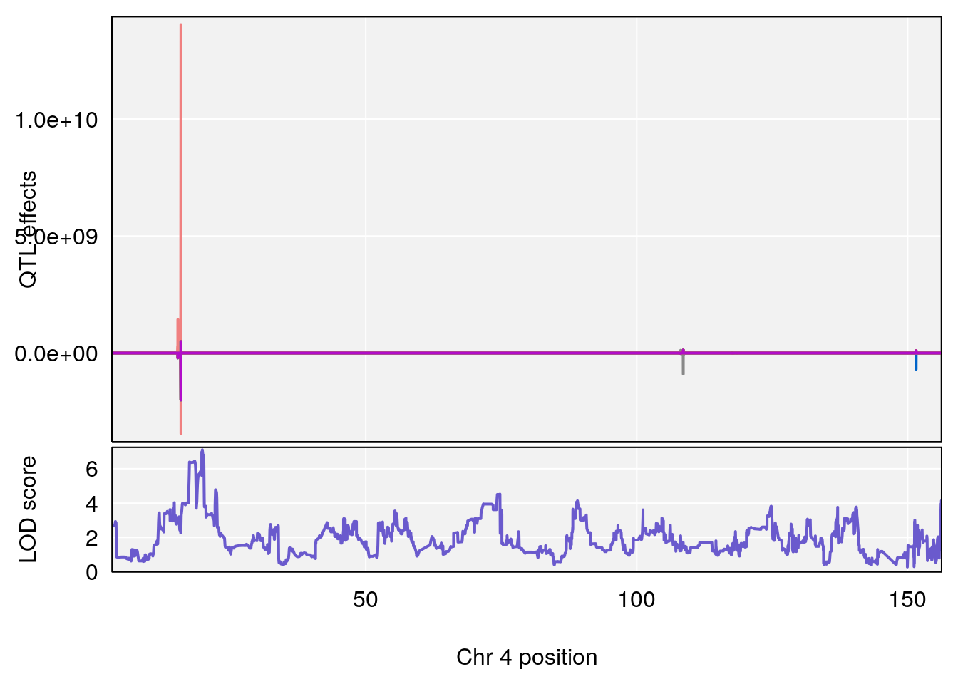
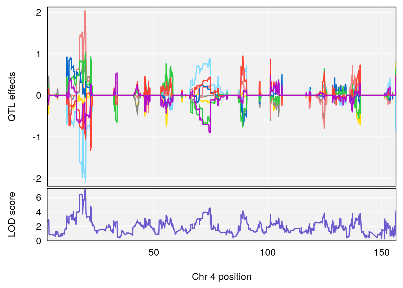
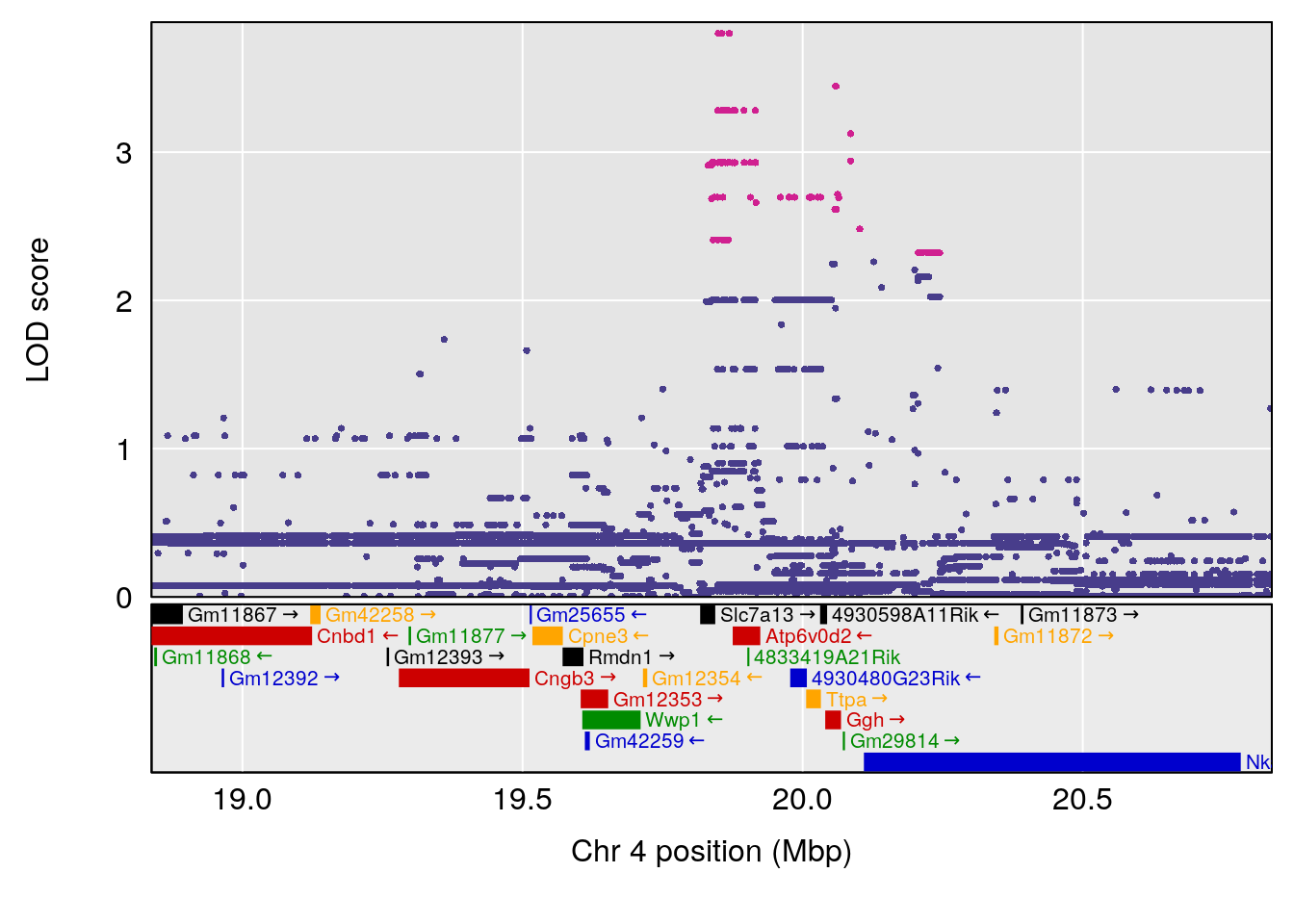
# [1] 2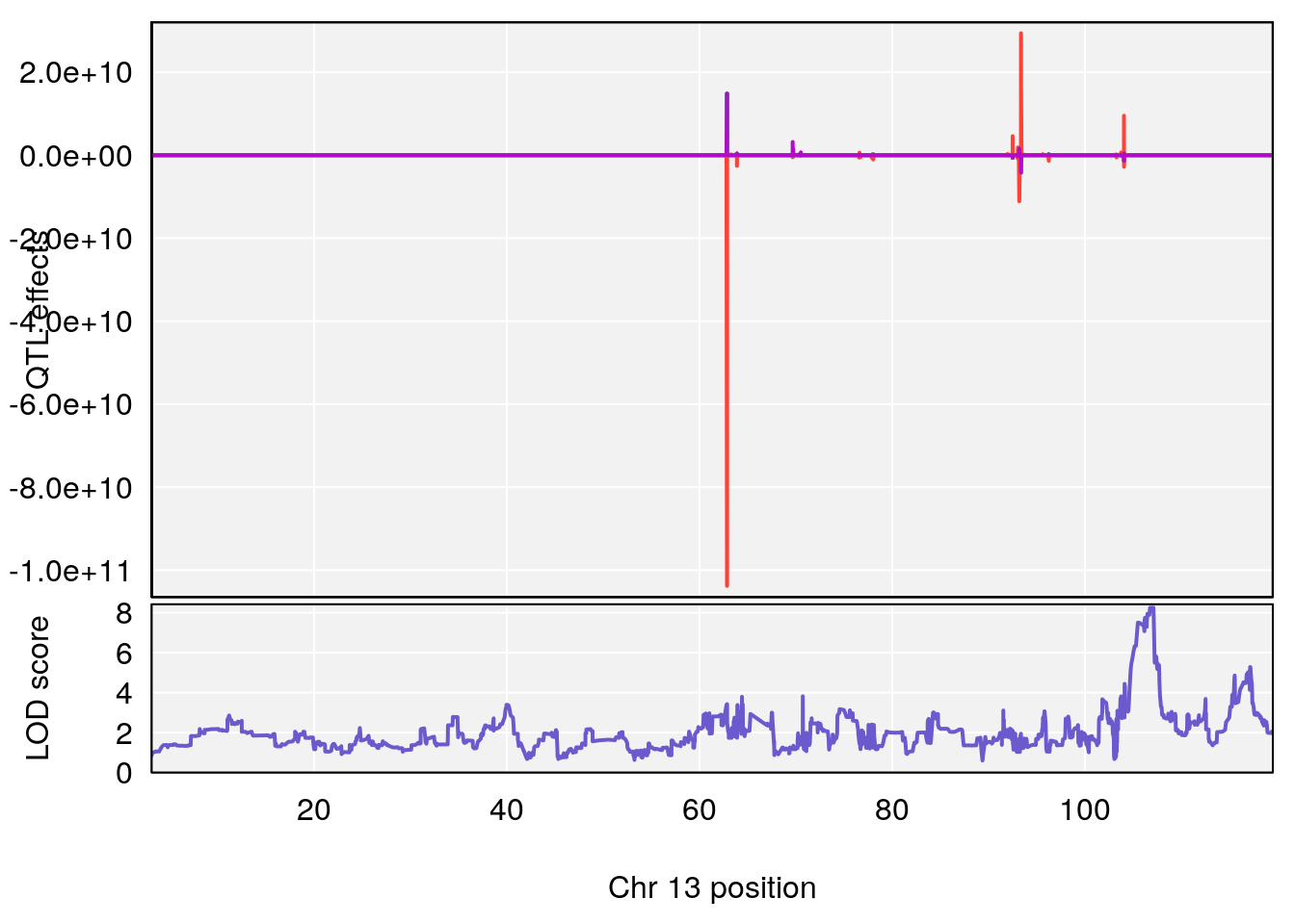
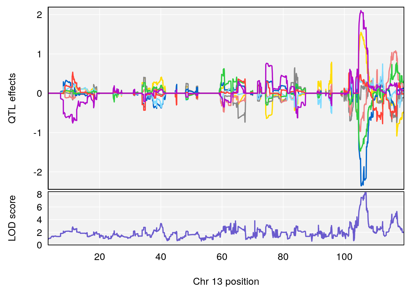
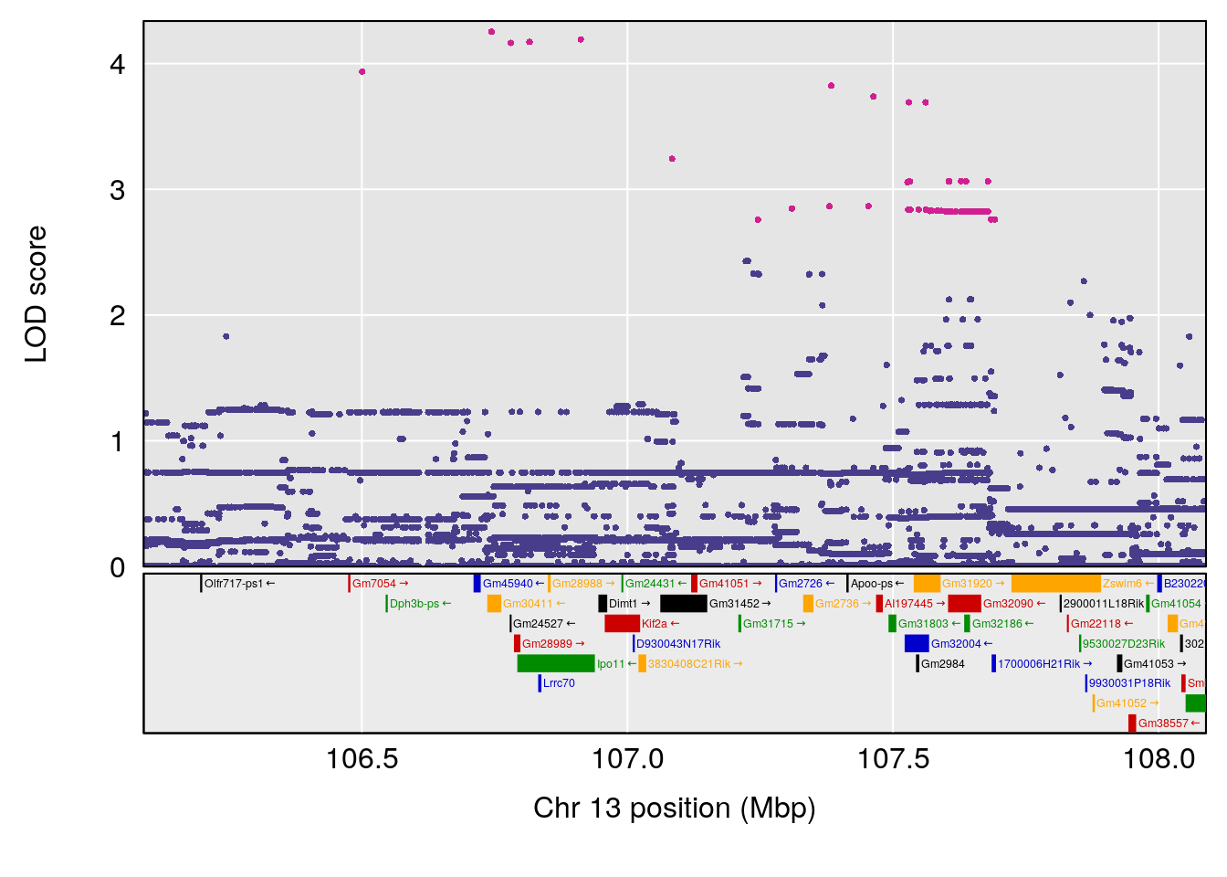
# [1] 3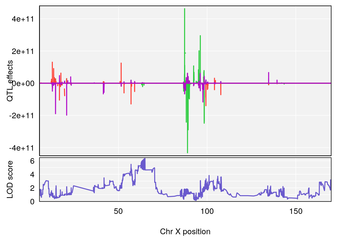
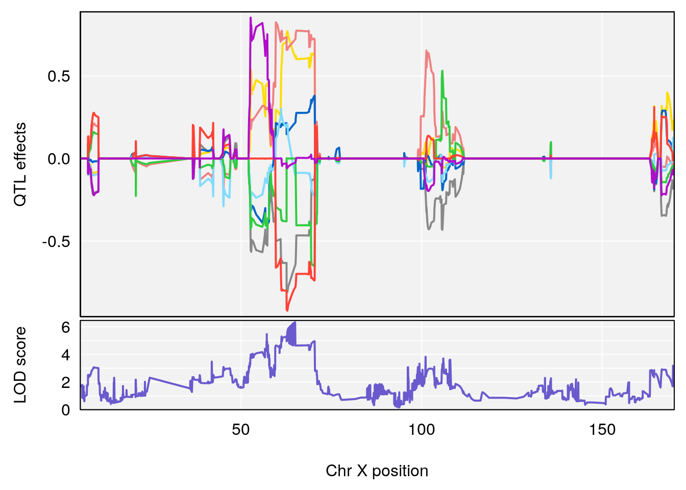
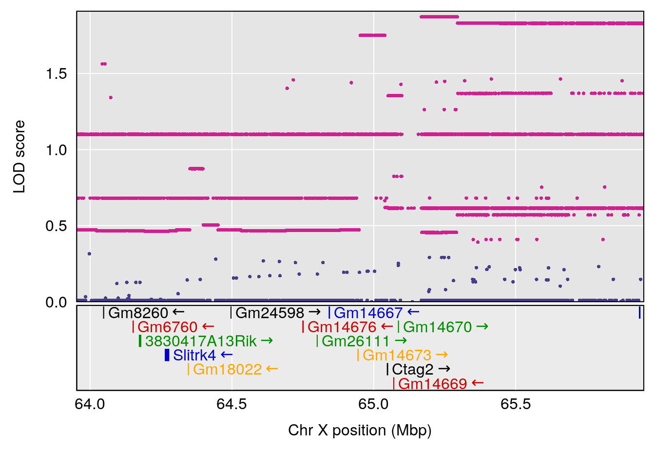
# [1] "Min.depression"
#   lodindex lodcolumn chr      pos      lod    ci_lo    ci_hi
# 1        1    pheno1   6 124.4987 6.178658 122.7586 125.6617
# [1] 1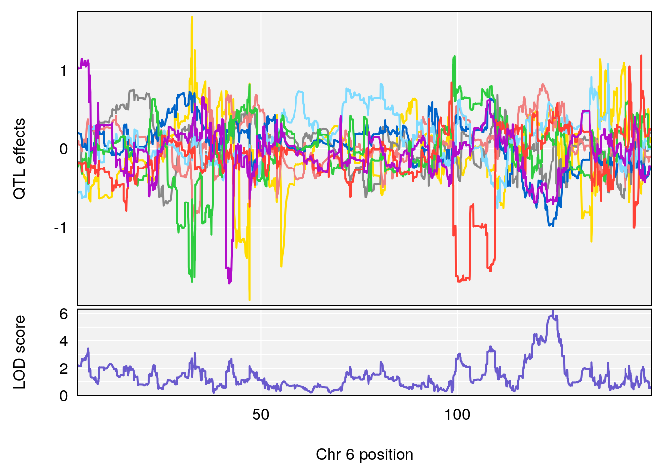
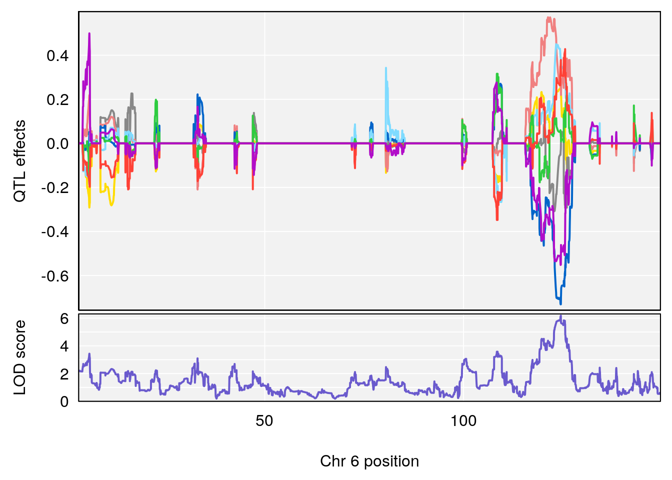
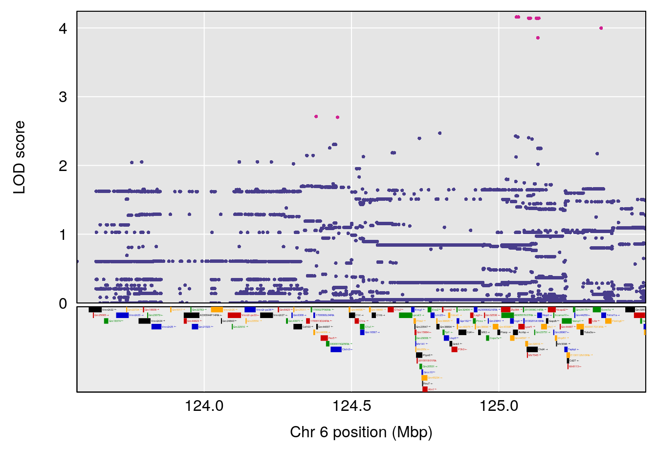
# [1] "Status_bin"
#   lodindex lodcolumn chr       pos      lod    ci_lo     ci_hi
# 1        1    pheno1   4  53.10525 6.807993 51.94764  54.94594
# 2        1    pheno1  10  95.60273 6.789714 94.90744  96.12668
# 3        1    pheno1  11  22.05810 6.923695 22.03080  22.07151
# 4        1    pheno1  12 119.97420 6.692607 29.97305 120.01743
# [1] 1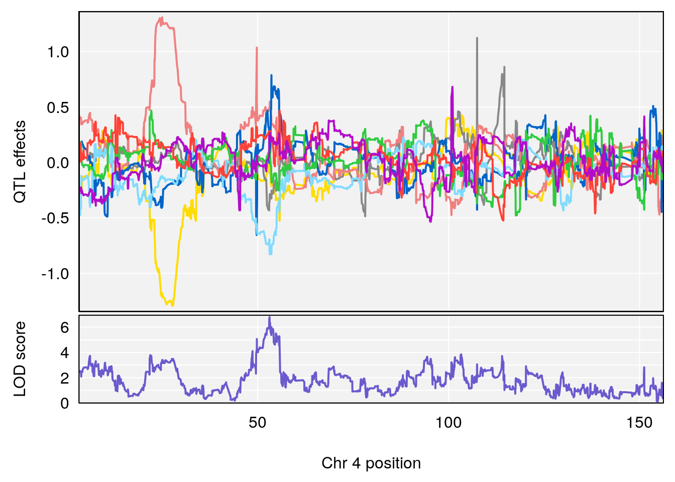
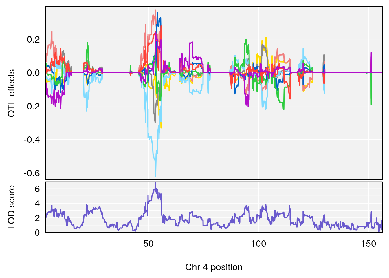

# [1] 2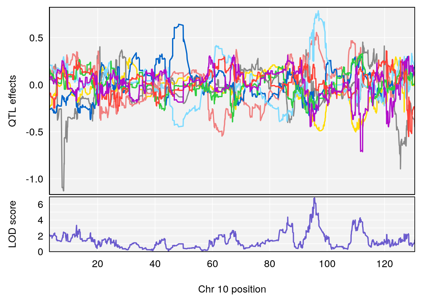
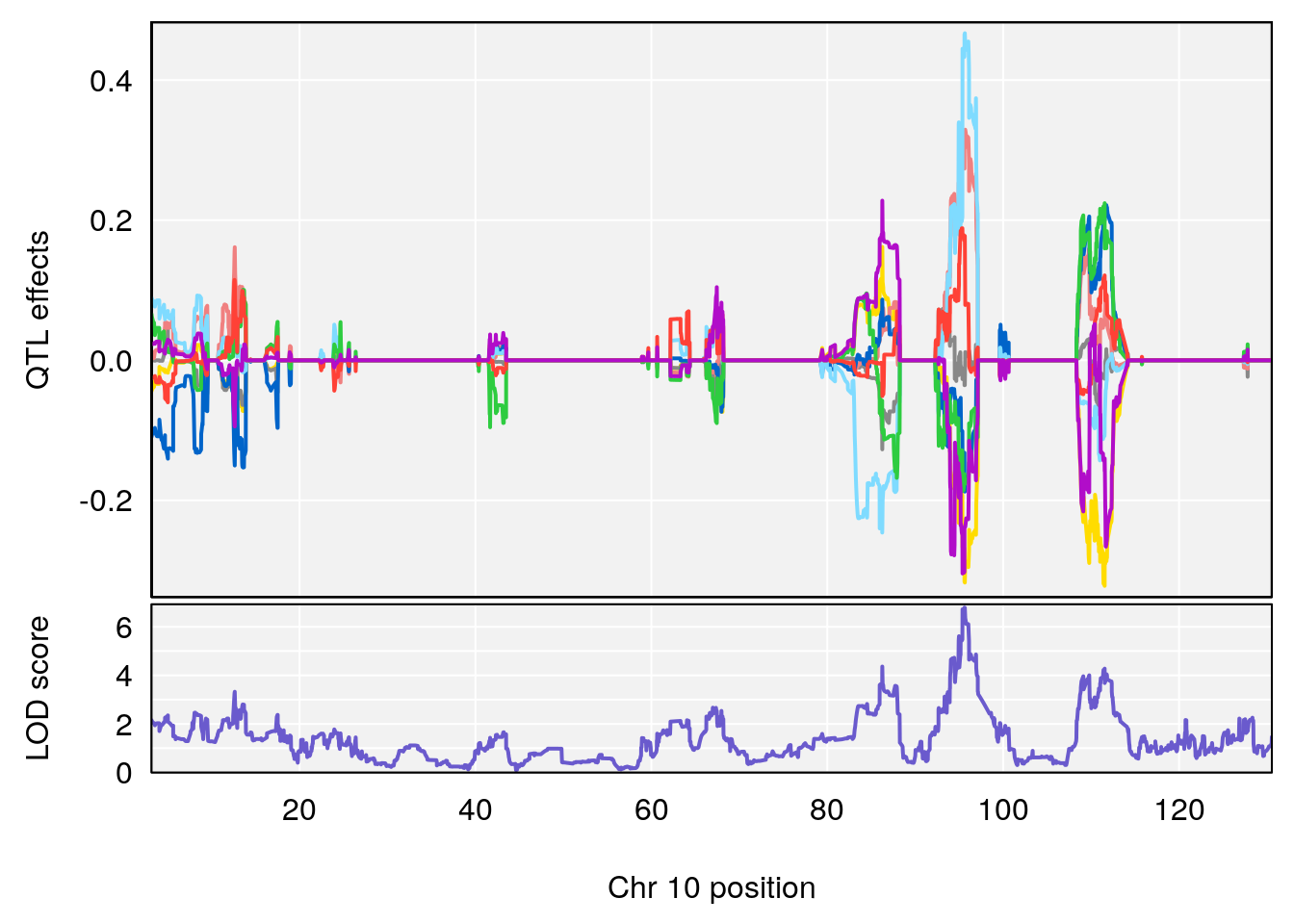
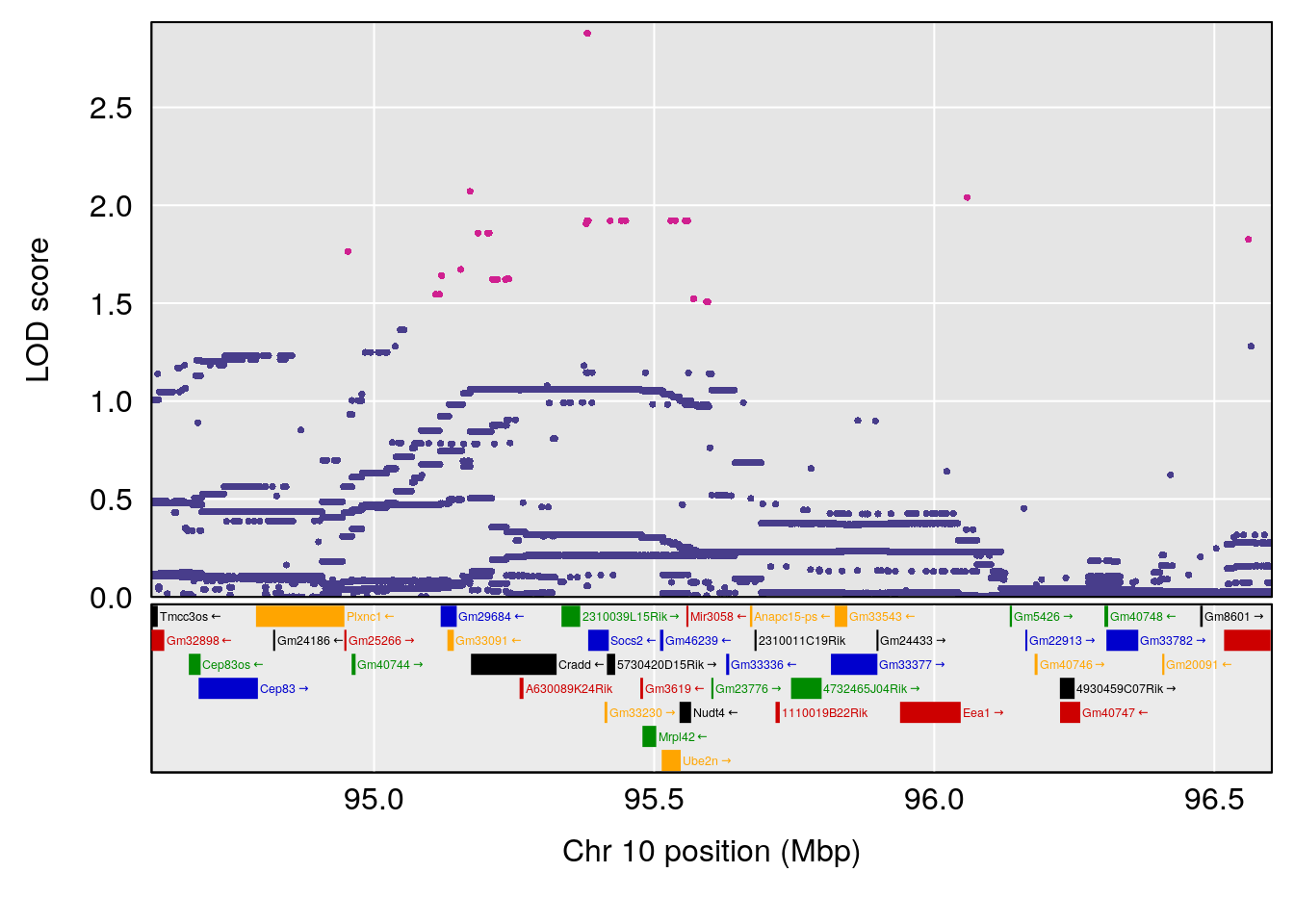
# [1] 3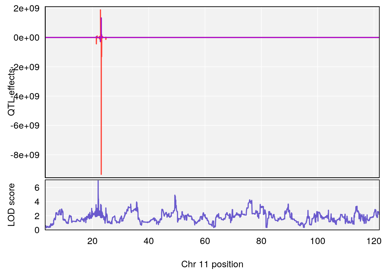
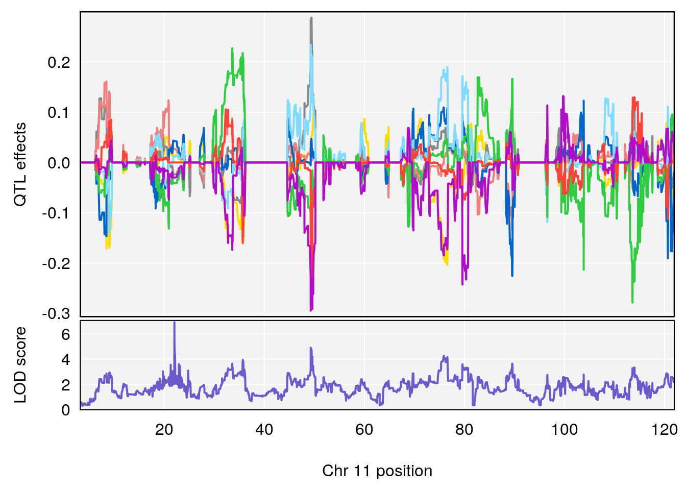
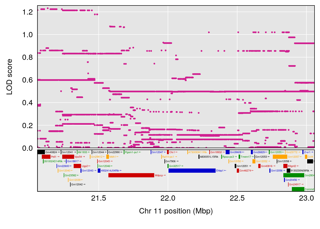
# [1] 4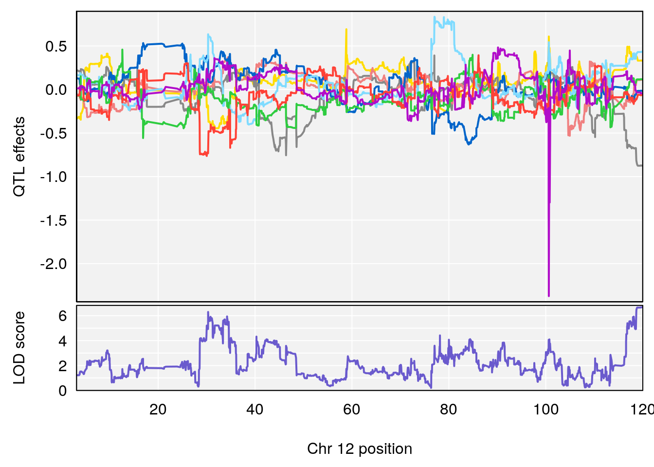
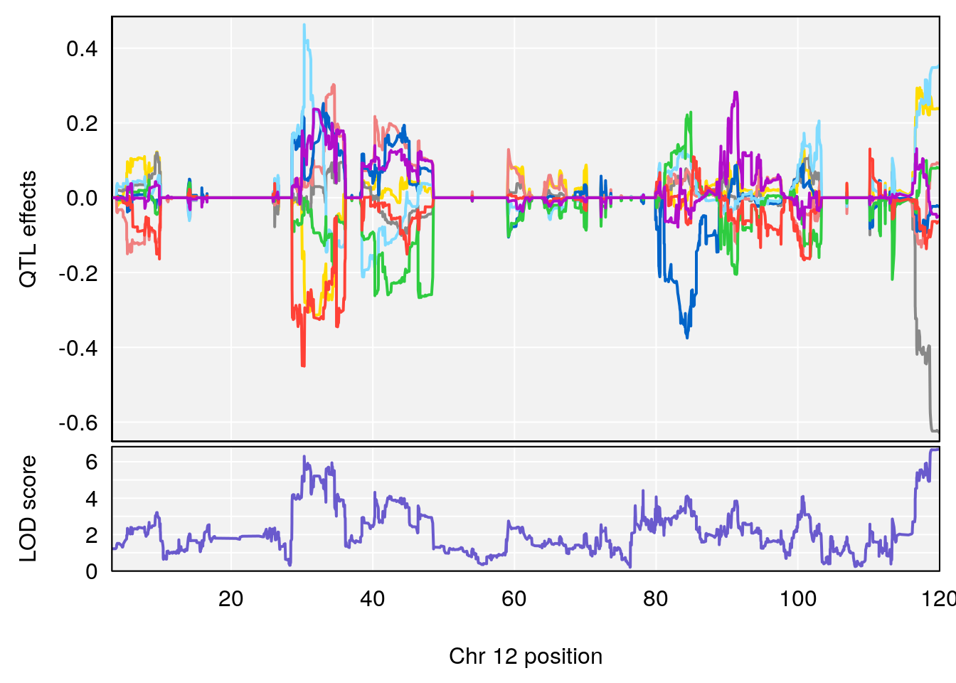
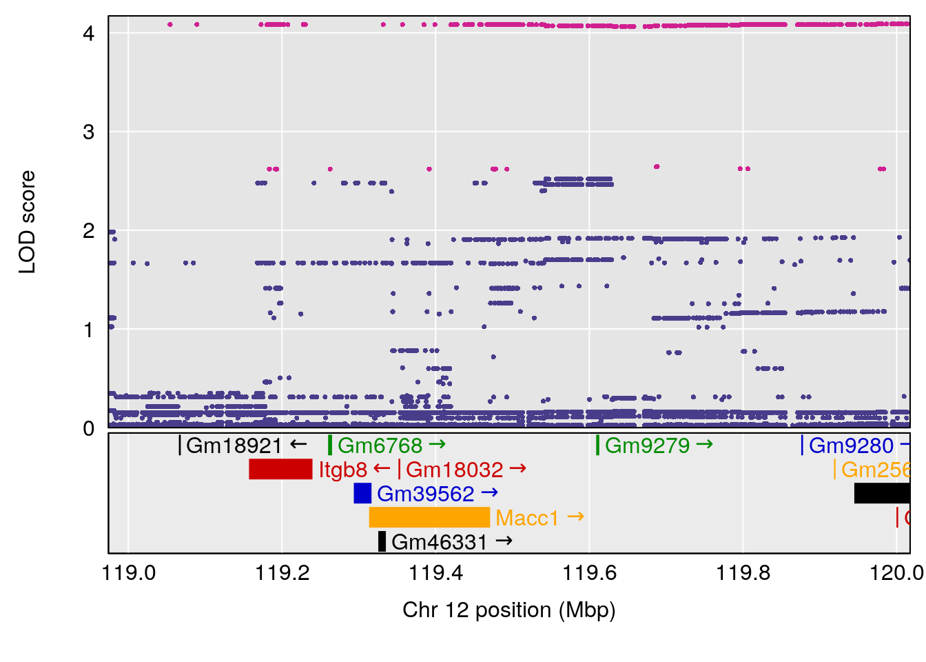
# [1] "f__Bpm"
#   lodindex lodcolumn chr      pos      lod   ci_lo    ci_hi
# 1        1    pheno1   1 149.9586 6.484401 127.387 150.3152
# [1] 1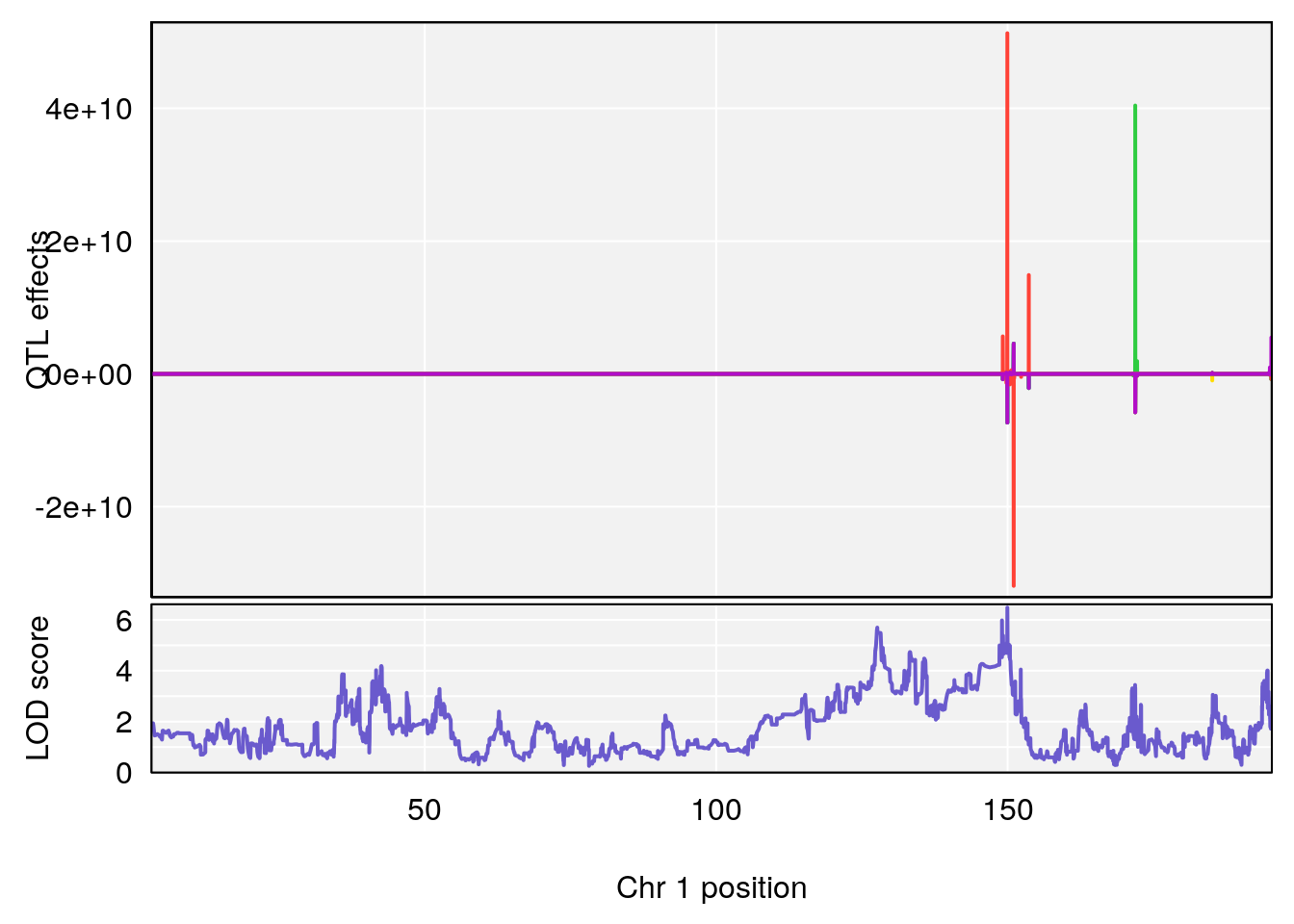
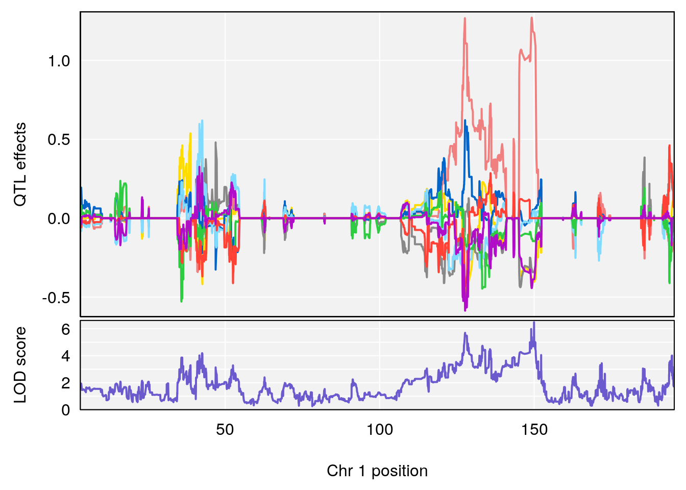
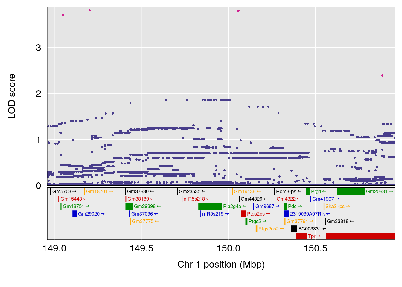
# [1] "TVb_ml"
#   lodindex lodcolumn chr      pos      lod  ci_lo    ci_hi
# 1        1    pheno1   6 6.099002 7.353069 5.9951 7.805745
# [1] 1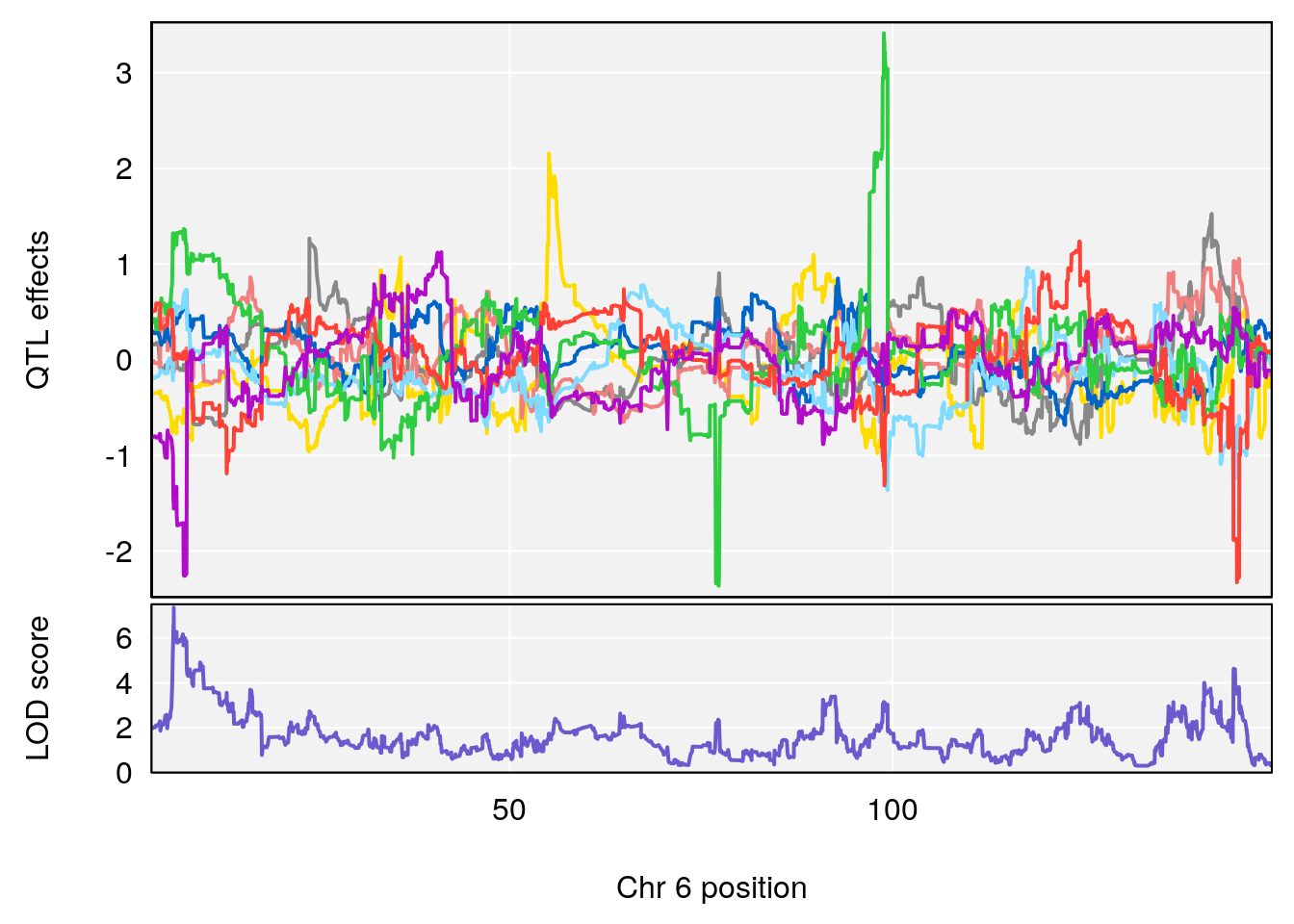
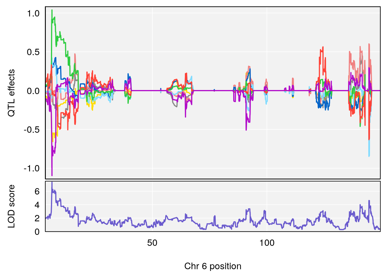
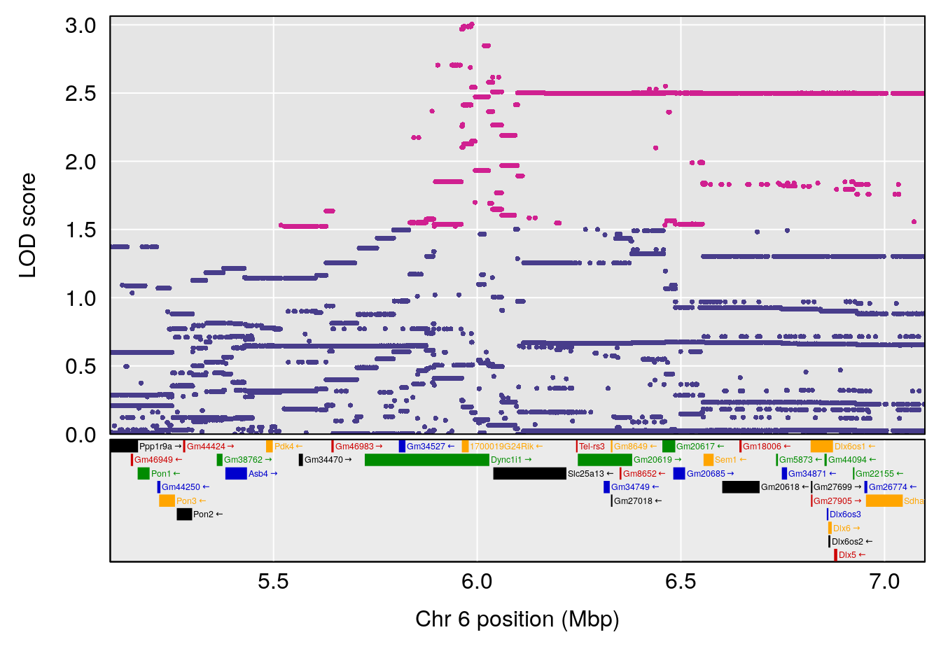
# [1] "MVb__ml_min"
#   lodindex lodcolumn chr      pos      lod    ci_lo    ci_hi
# 1        1    pheno1   2 31.31643 7.208511 30.96371 32.48273
# [1] 1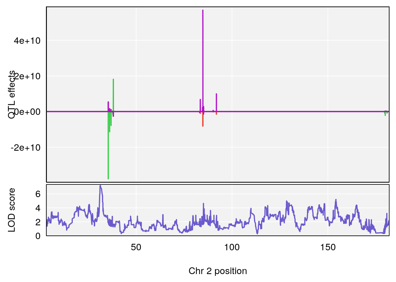
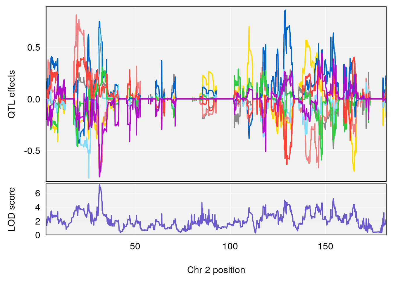
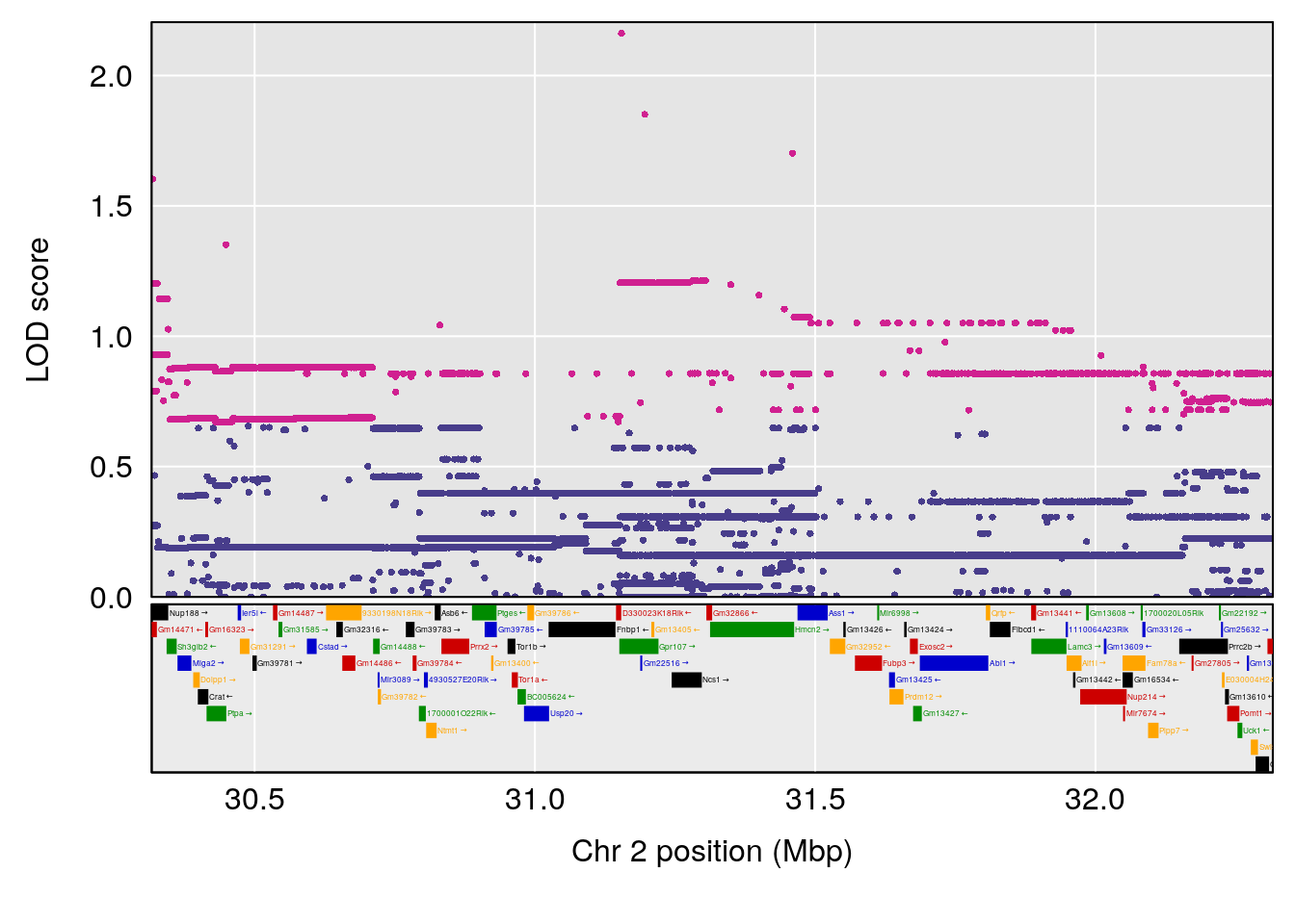
# [1] "Penh"
#   lodindex lodcolumn chr      pos      lod    ci_lo    ci_hi
# 1        1    pheno1  12 36.04641 6.535914 34.82905 36.14215
# 2        1    pheno1  17 77.55452 6.040561 76.68592 78.57356
# [1] 1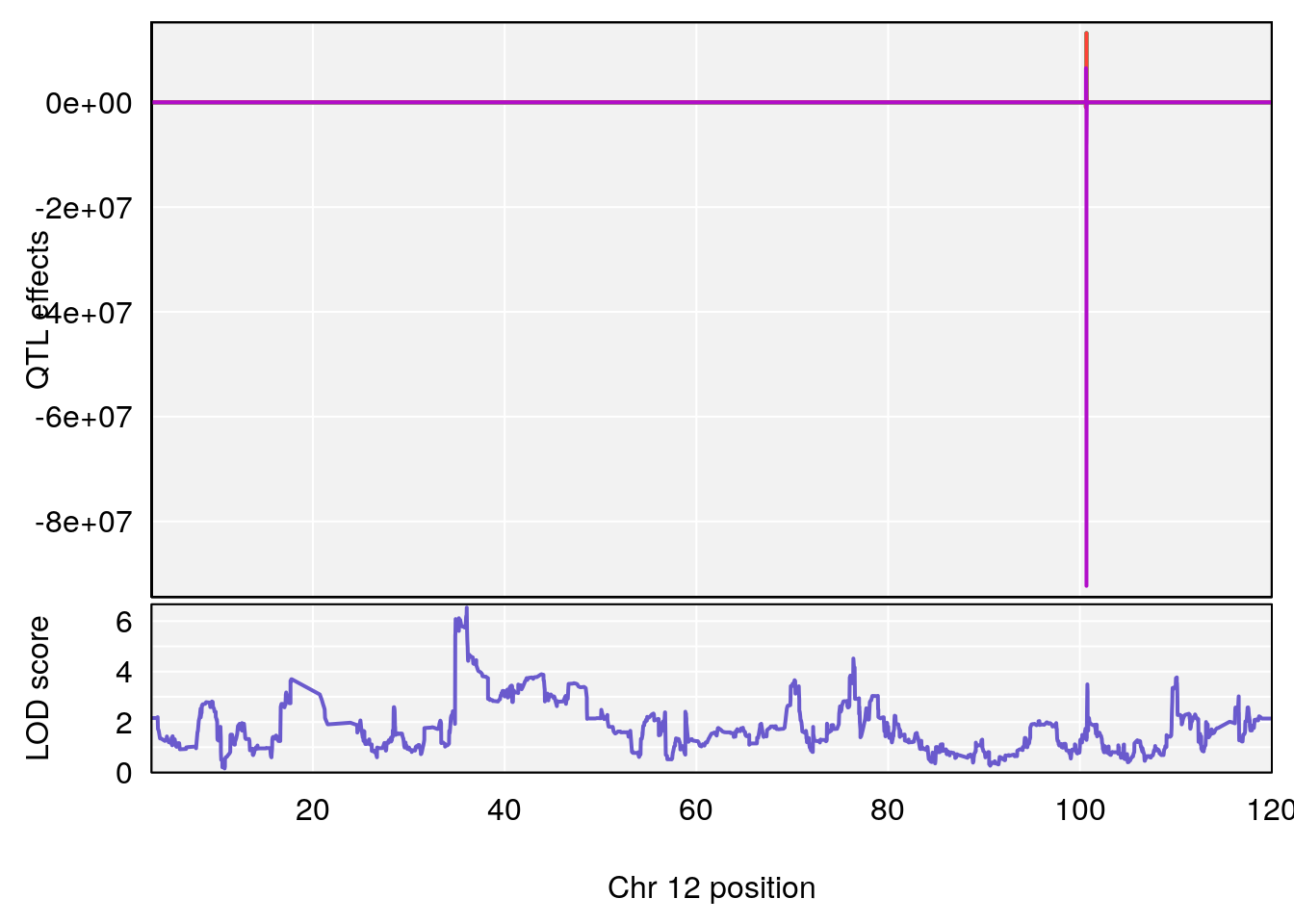
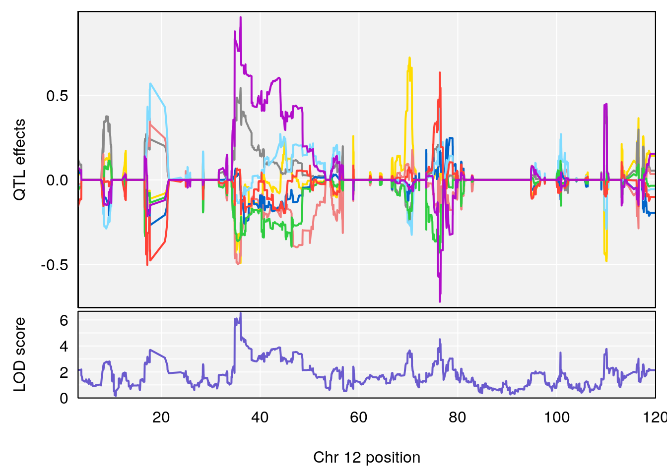
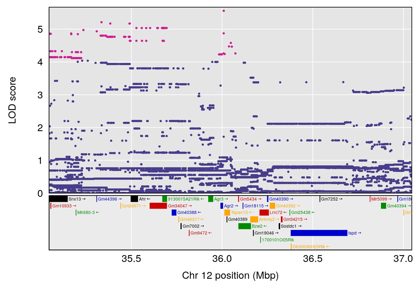
# [1] 2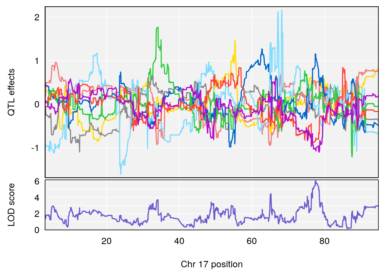
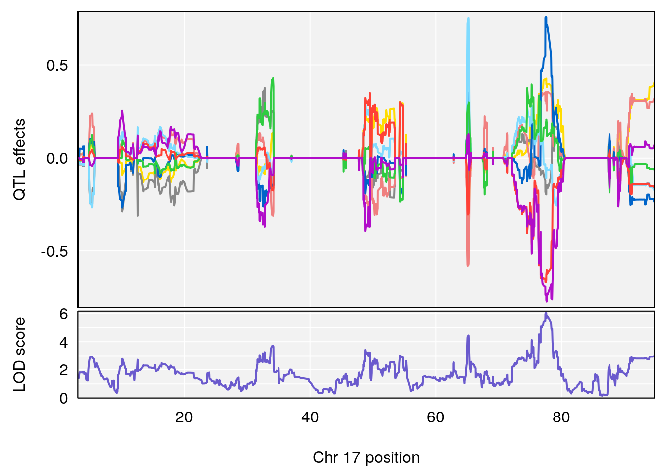
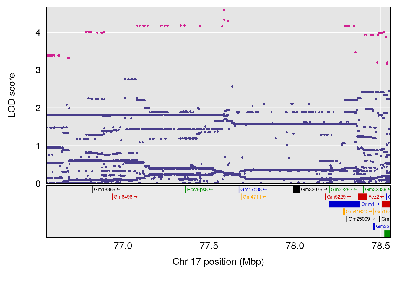
# [1] "PAU"
#   lodindex lodcolumn chr      pos      lod    ci_lo    ci_hi
# 1        1    pheno1  12 35.22826 6.041084 34.82905 36.14215
# [1] 1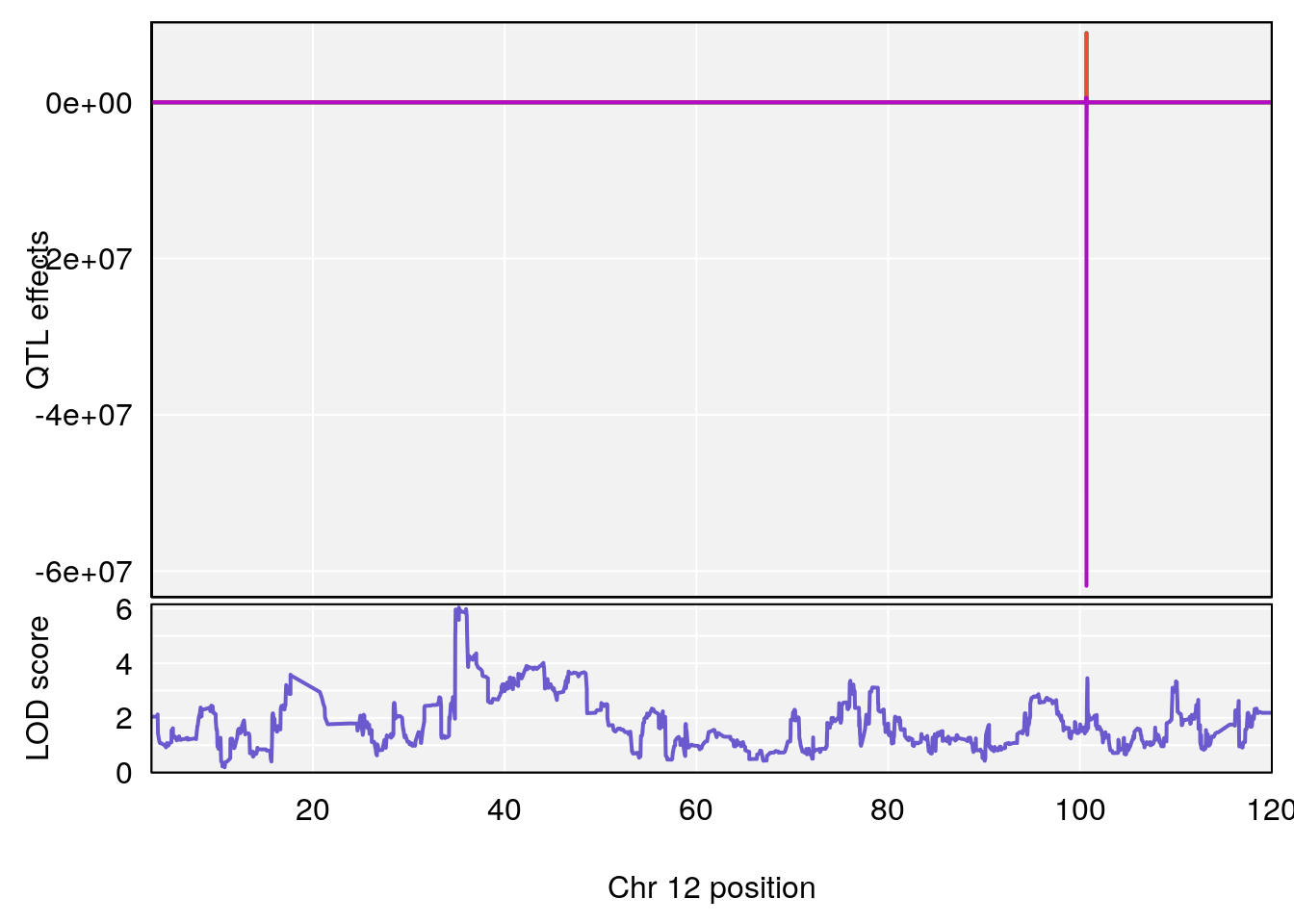
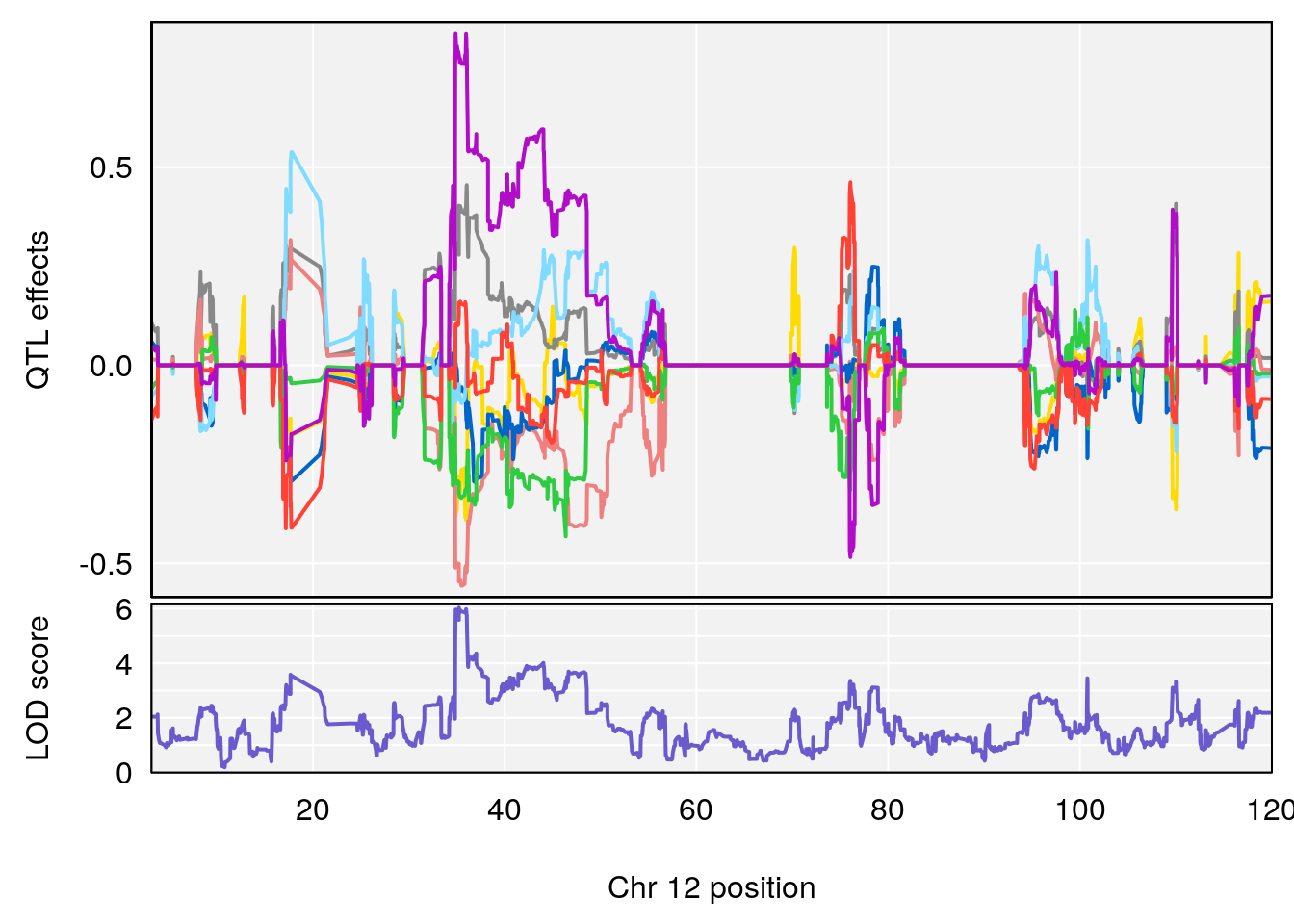
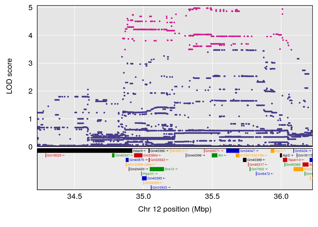
# [1] "Rpef"
# [1] lodindex  lodcolumn chr       pos       lod       ci_lo     ci_hi
# <0 rows> (or 0-length row.names)
# [1] "PIFb"
#   lodindex lodcolumn chr     pos      lod    ci_lo     ci_hi
# 1        1    pheno1   2 31.3284 6.974314 30.96371 154.21302
# 2        1    pheno1  18 81.4866 6.089970 60.96035  81.78568
# [1] 1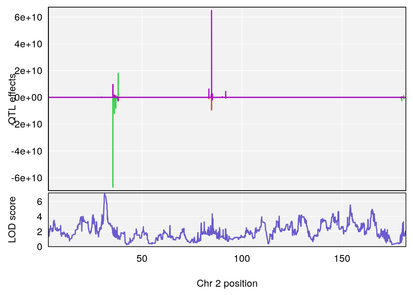
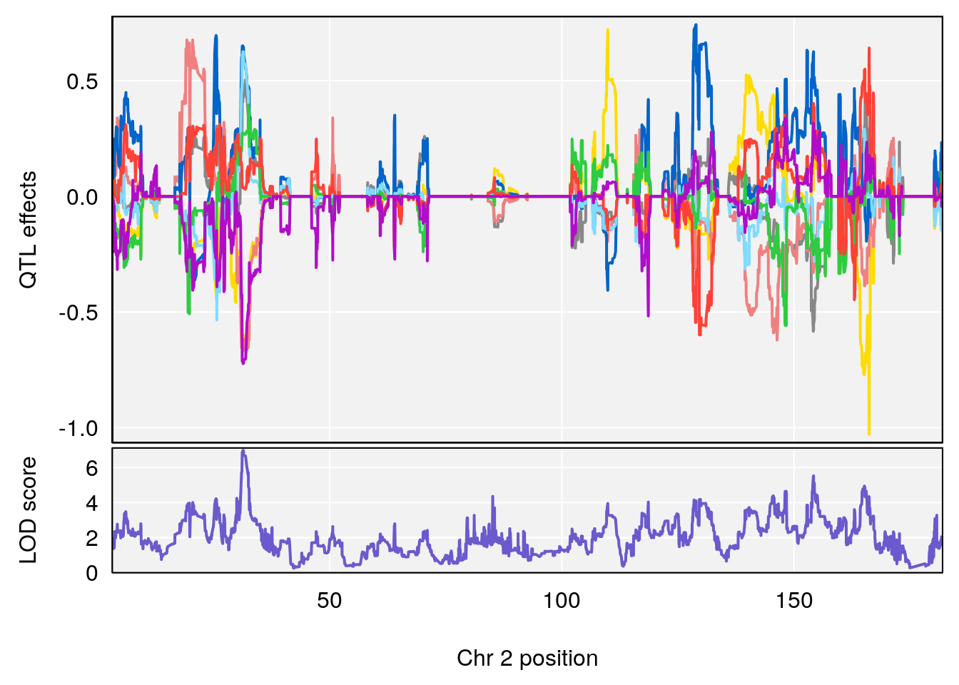
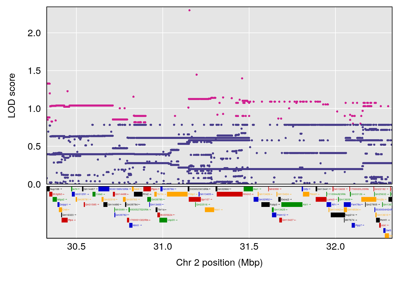
# [1] 2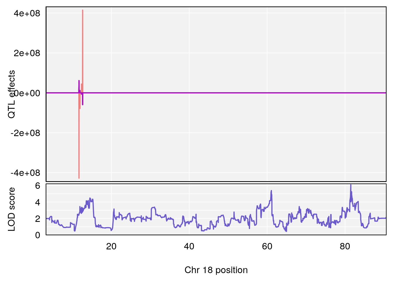
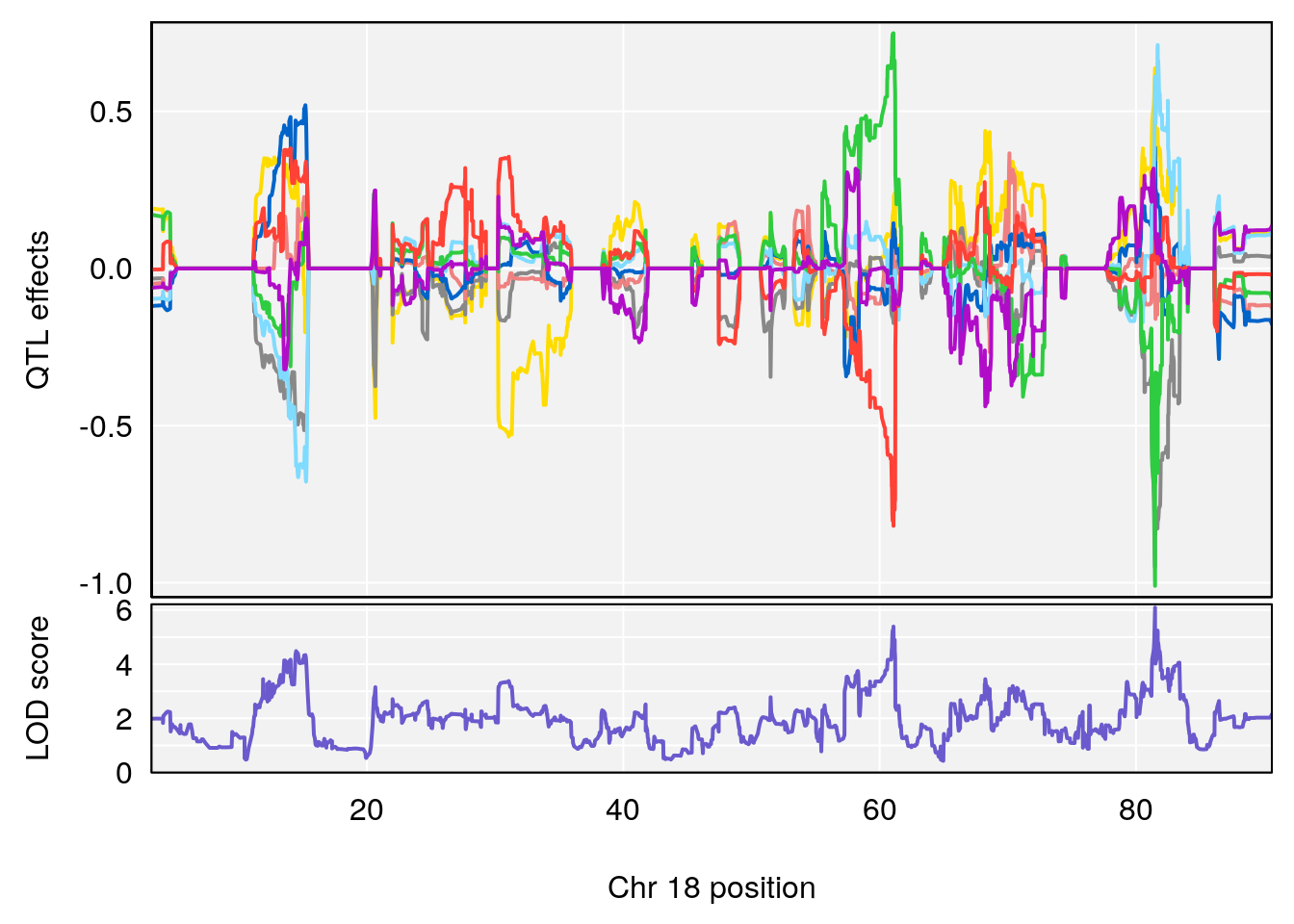
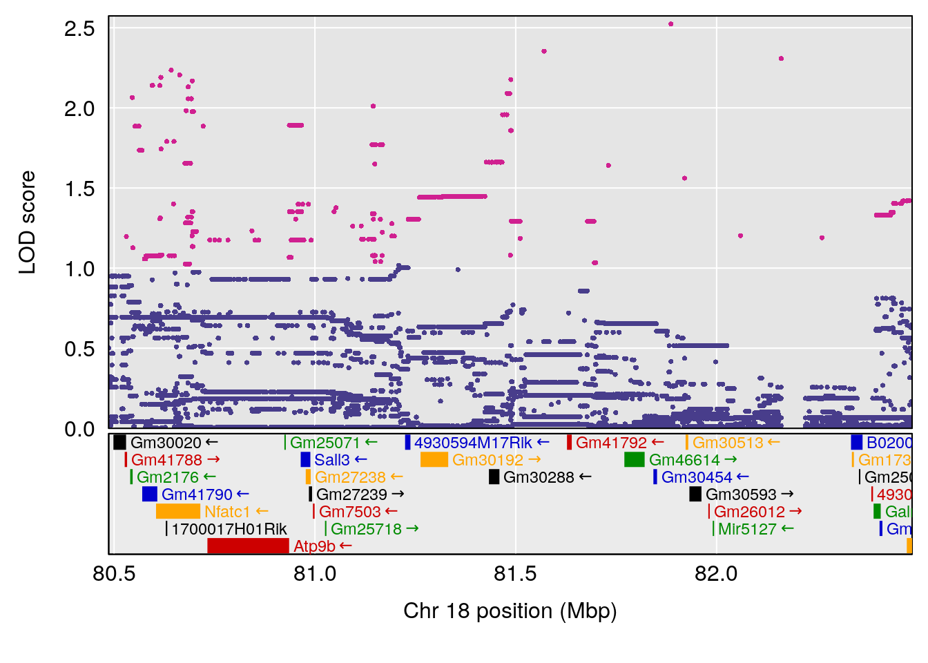
# [1] "PEFb"
#   lodindex lodcolumn chr      pos      lod    ci_lo    ci_hi
# 1        1    pheno1   2 31.42209 7.596845 30.97043 32.37755
# 2        1    pheno1  18 61.04847 6.116981 58.11397 81.69993
# [1] 1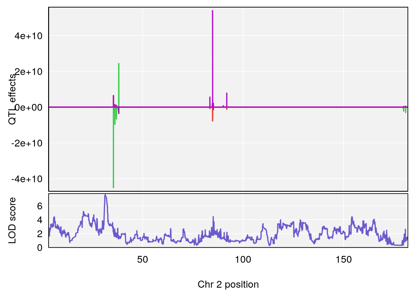
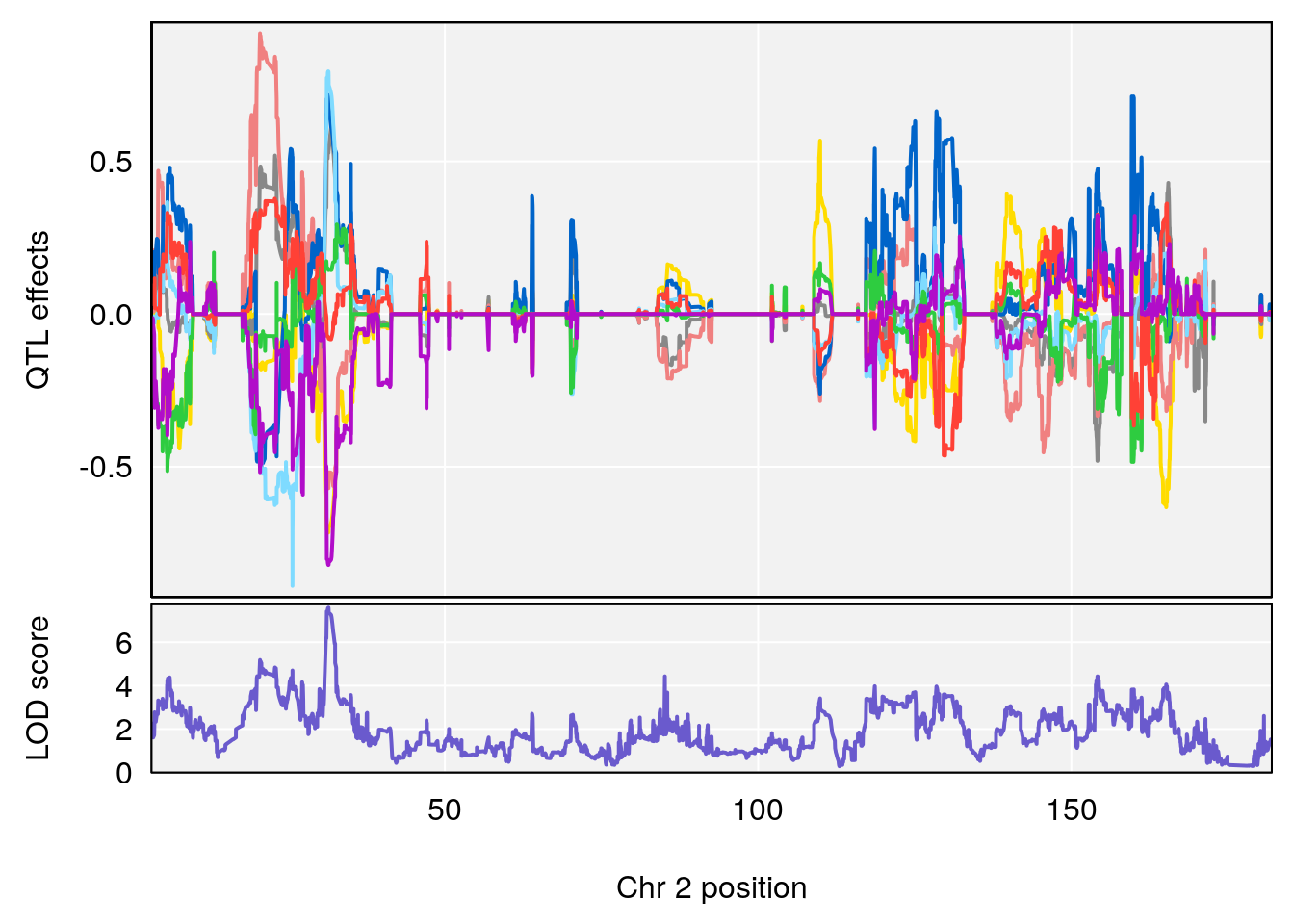
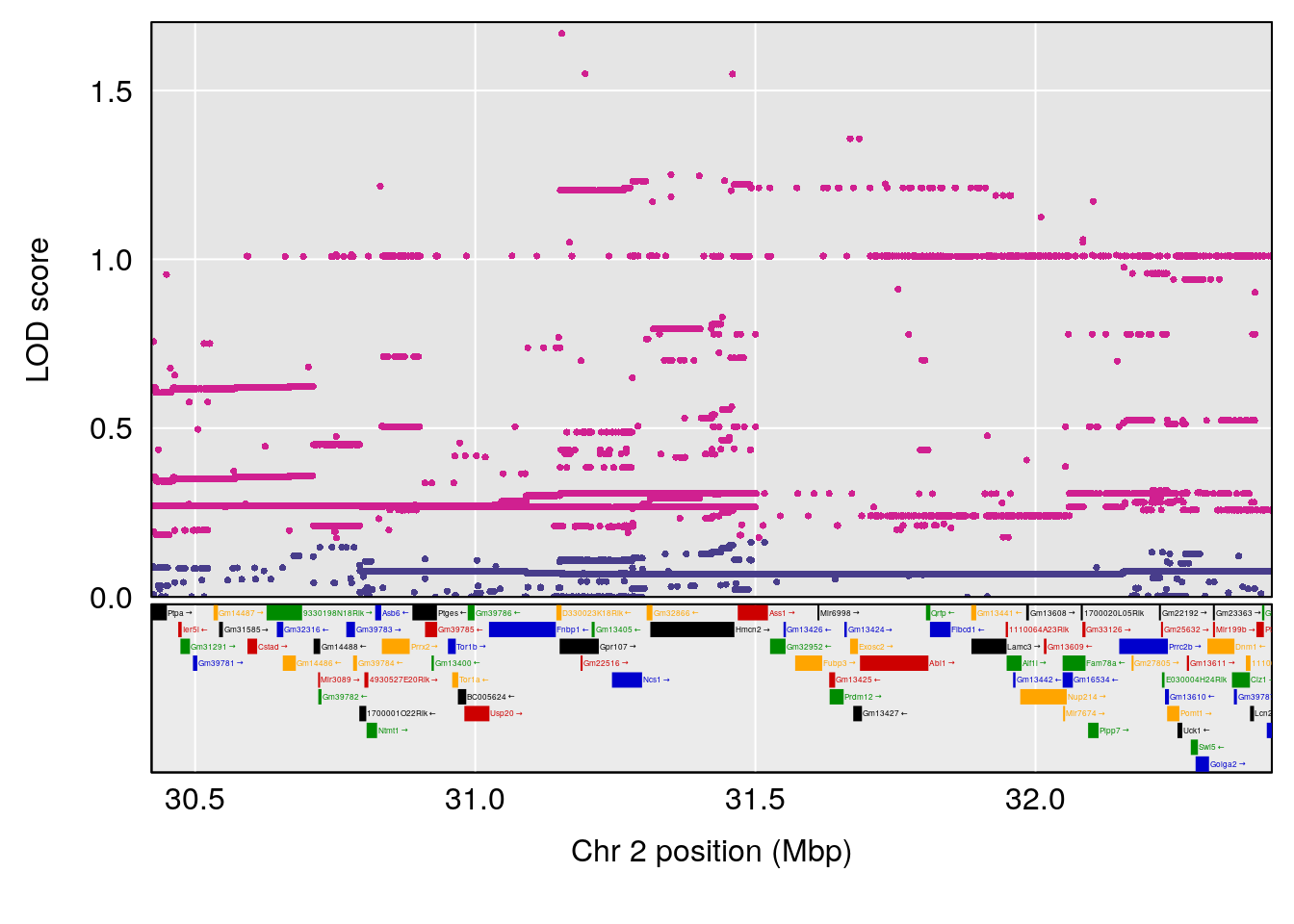
# [1] 2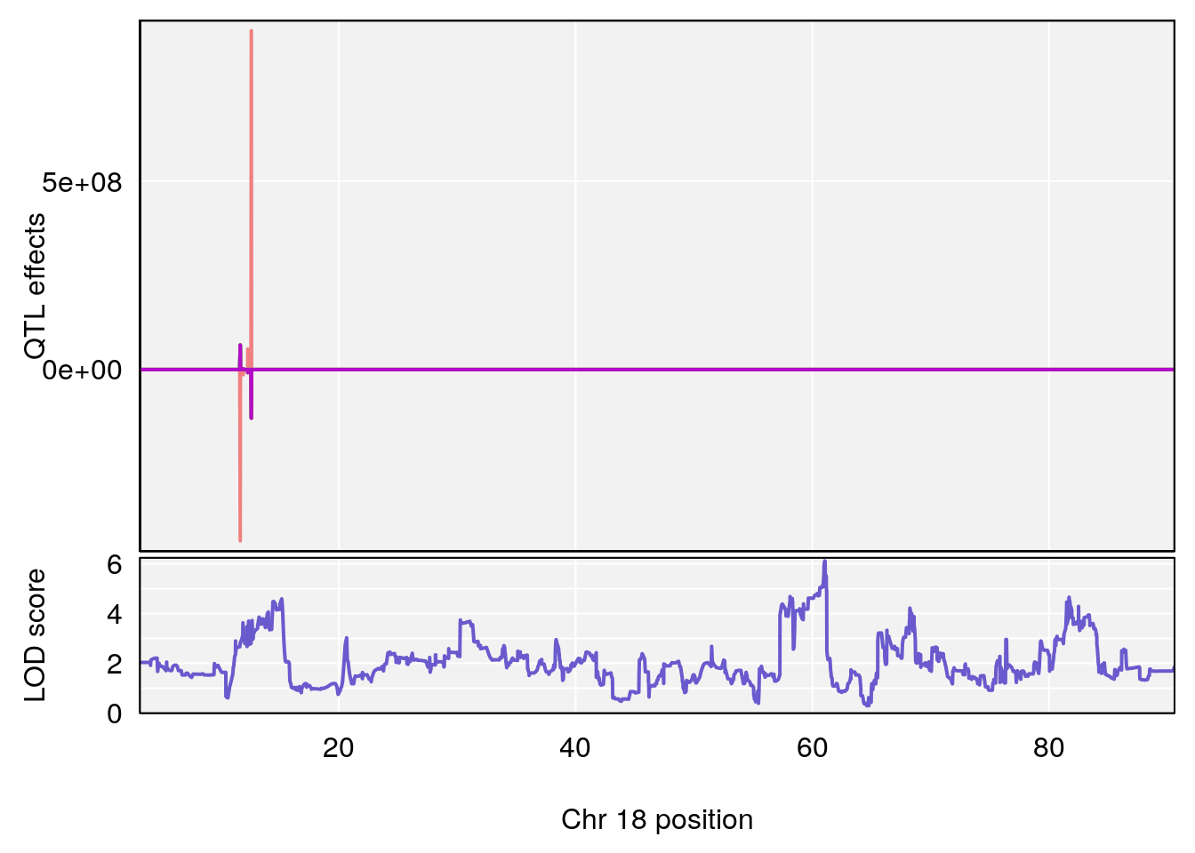
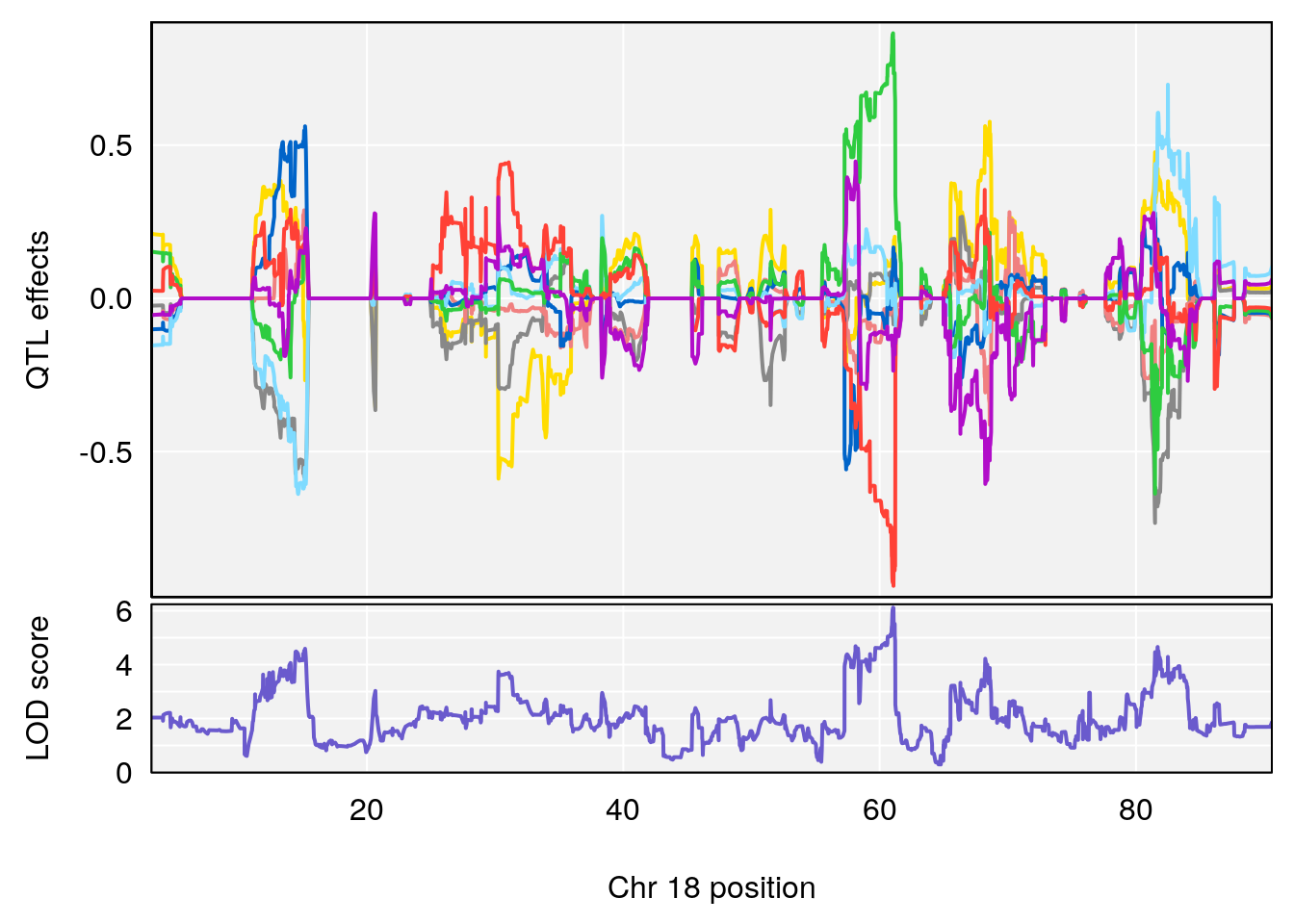
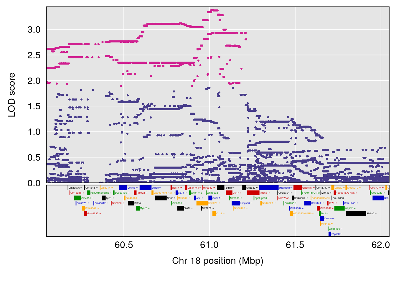
# [1] "Ti__sec"
#   lodindex lodcolumn chr       pos      lod     ci_lo    ci_hi
# 1        1    pheno1   1 149.95720 6.066942 127.22657 150.4074
# 2        1    pheno1   X  97.36966 6.097108  97.27061 101.1009
# [1] 1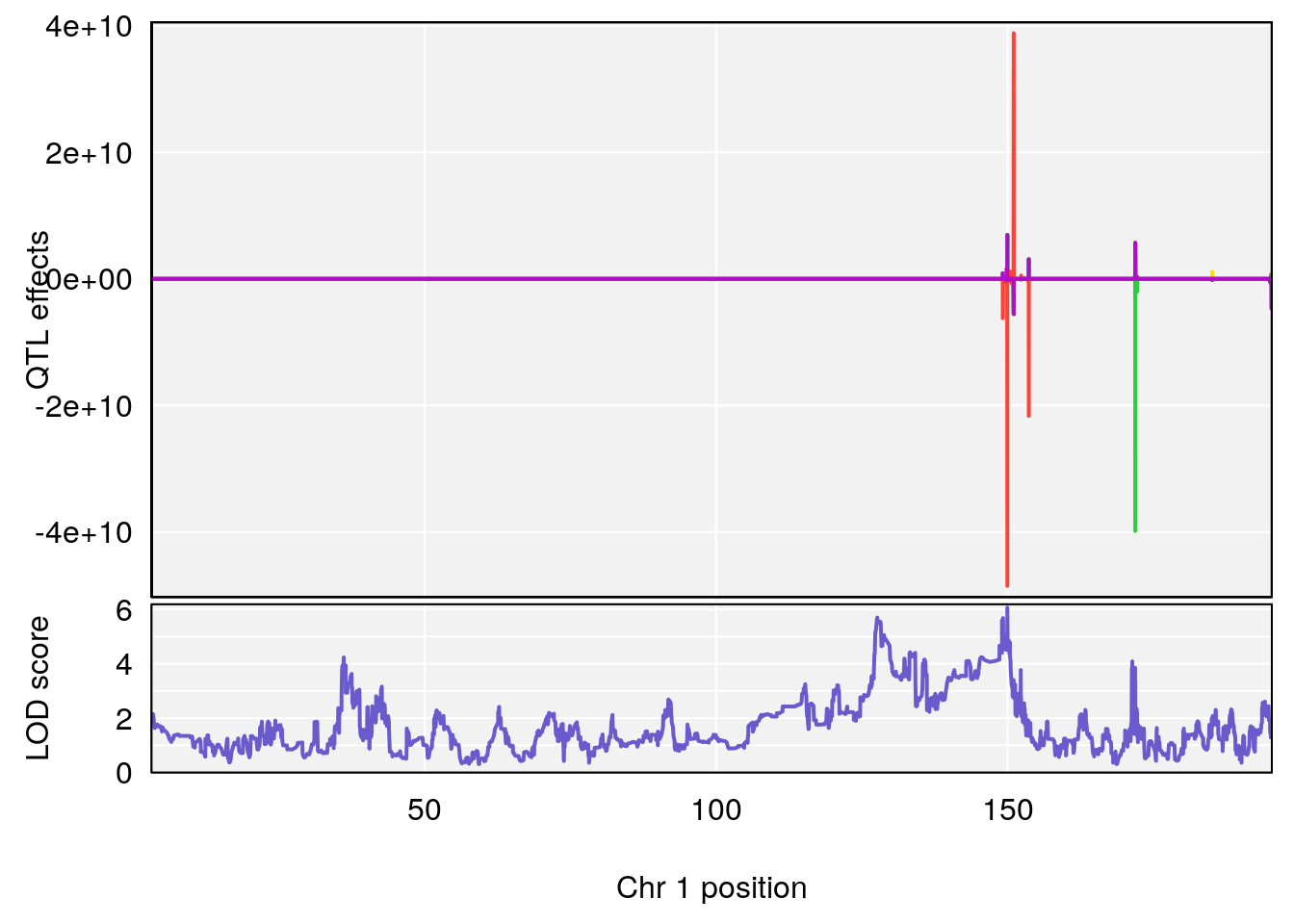
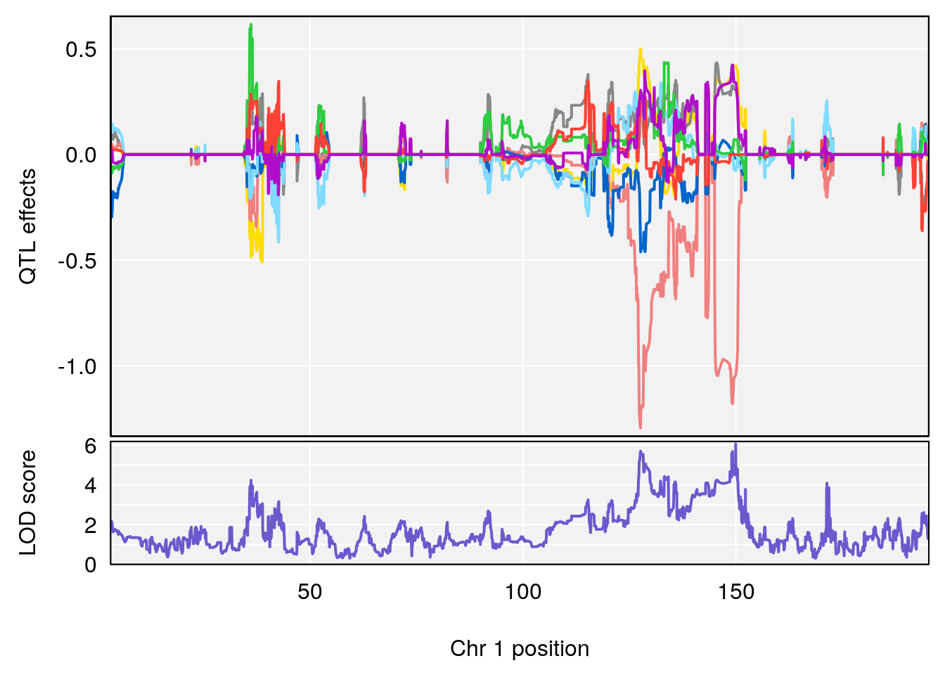
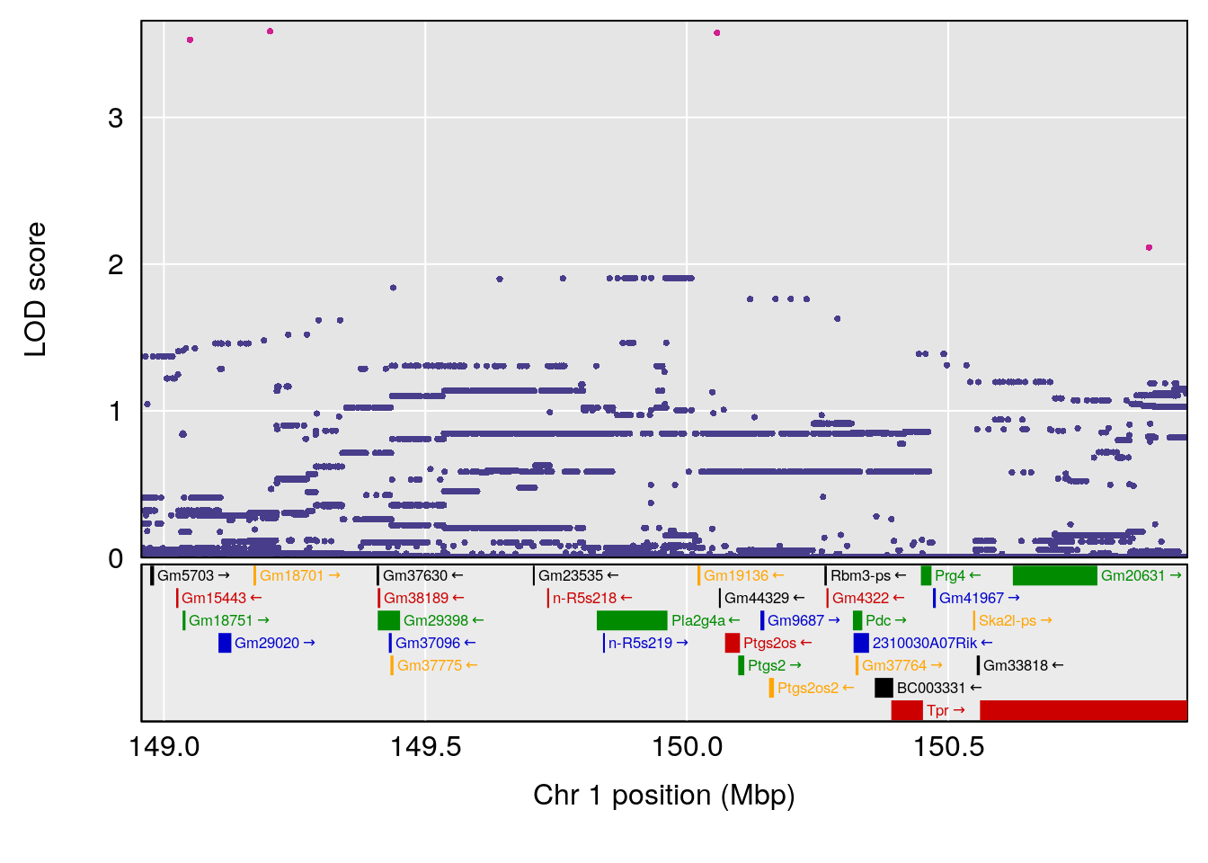
# [1] 2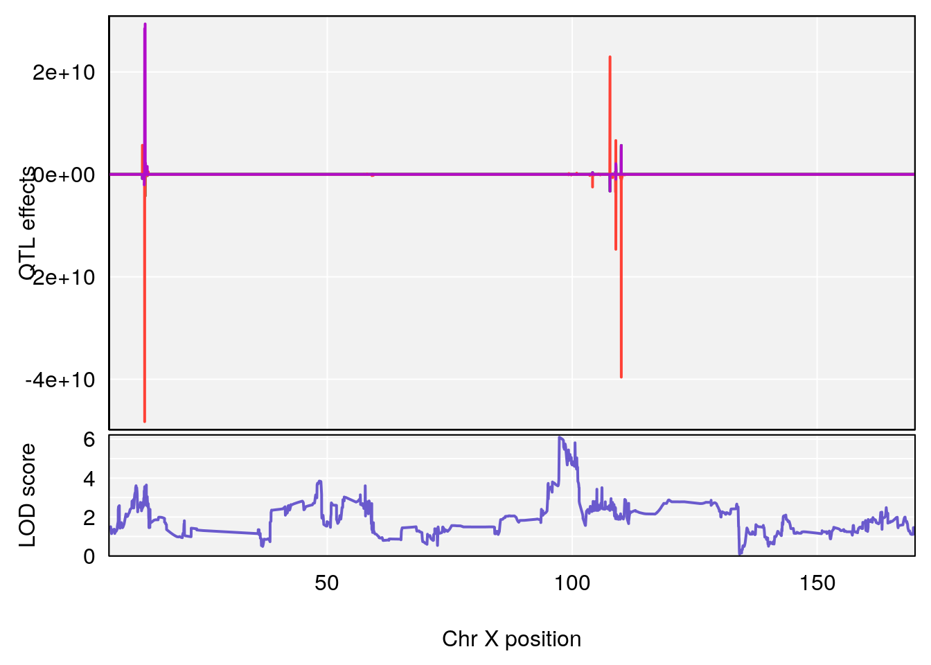
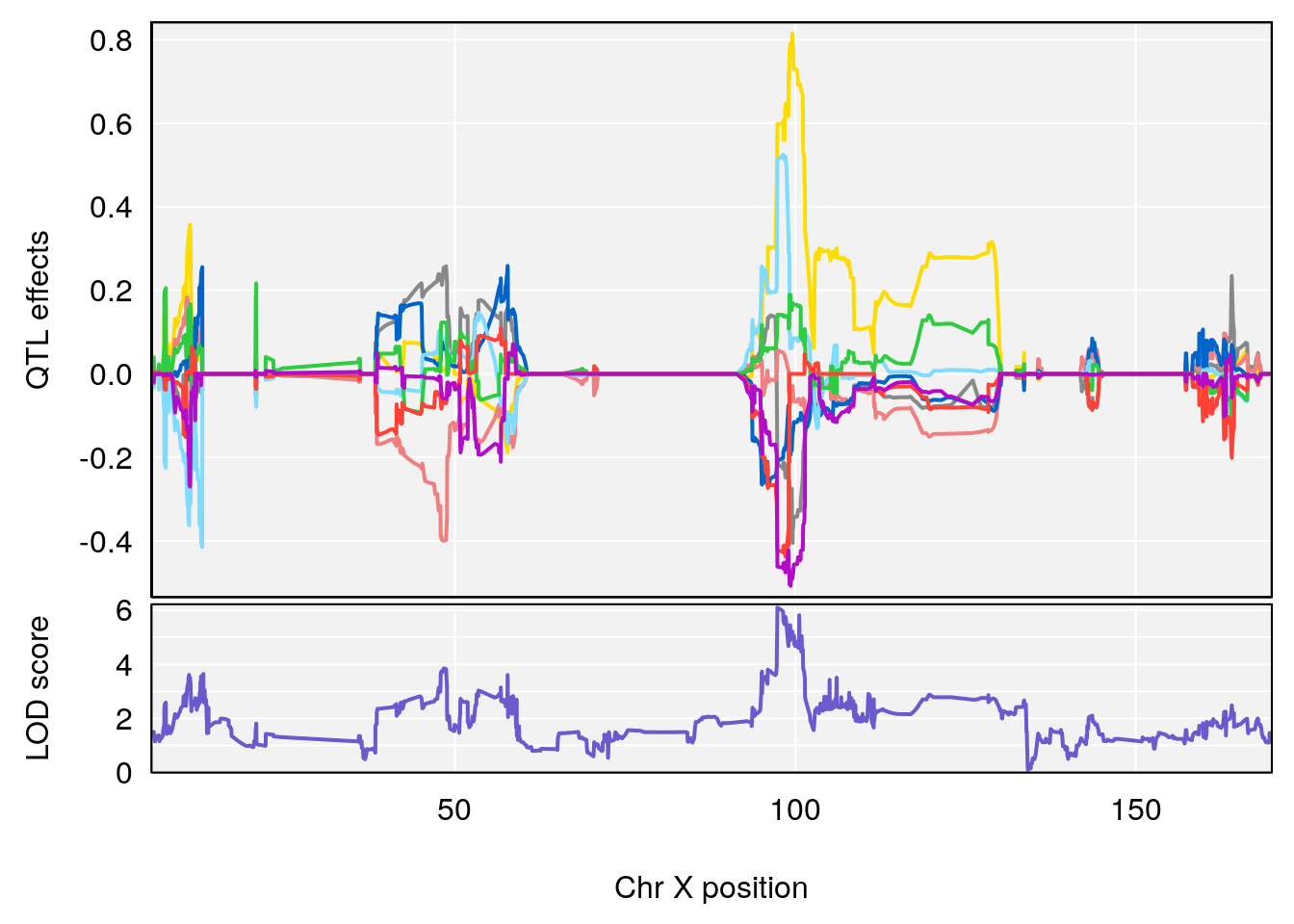
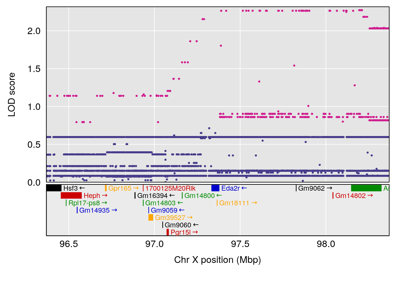
# [1] "Te__sec"
#   lodindex lodcolumn chr      pos      lod    ci_lo    ci_hi
# 1        1    pheno1  15 97.60229 6.586641 96.83978 97.66134
# [1] 1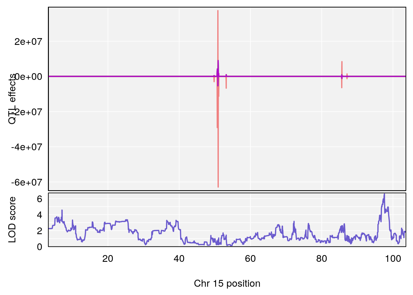
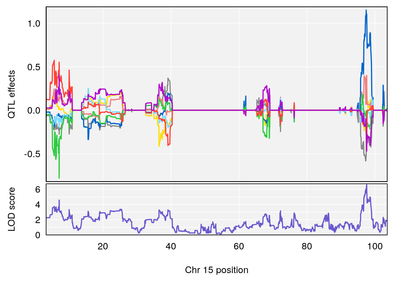
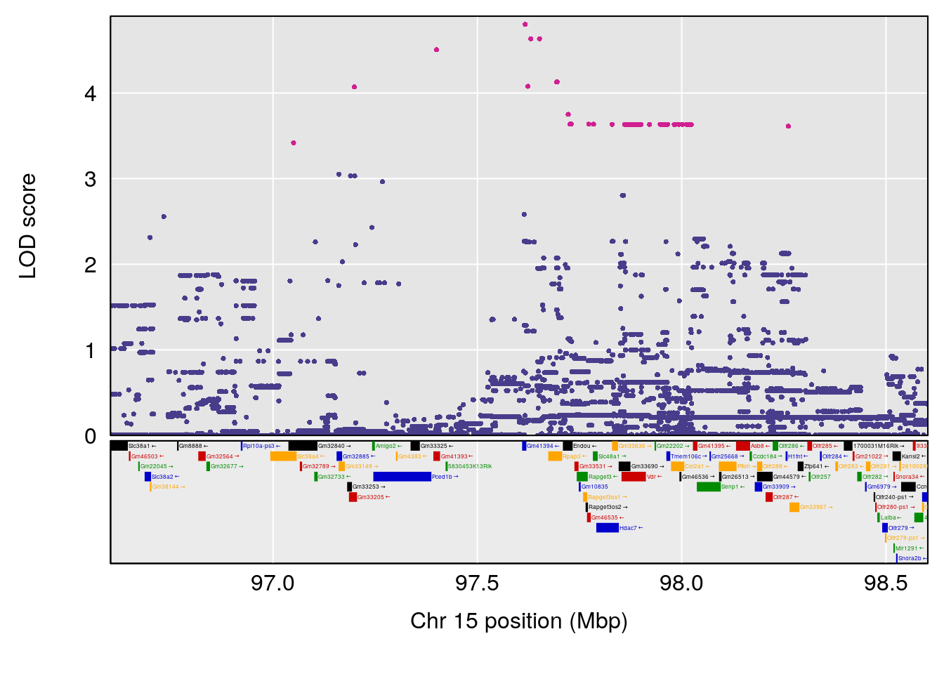
# [1] "EF50"
#   lodindex lodcolumn chr      pos      lod     ci_lo     ci_hi
# 1        1    pheno1   2 31.31365 6.241214 30.897328 154.21302
# 2        1    pheno1  15 86.28693 6.024603  7.093825  86.37266
# [1] 1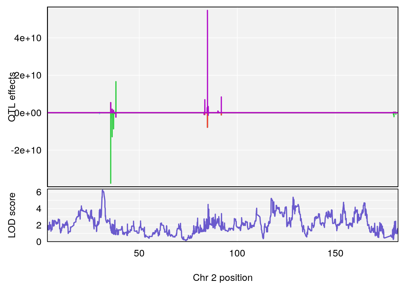
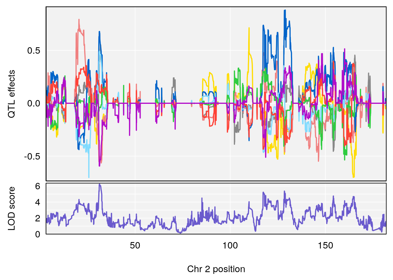
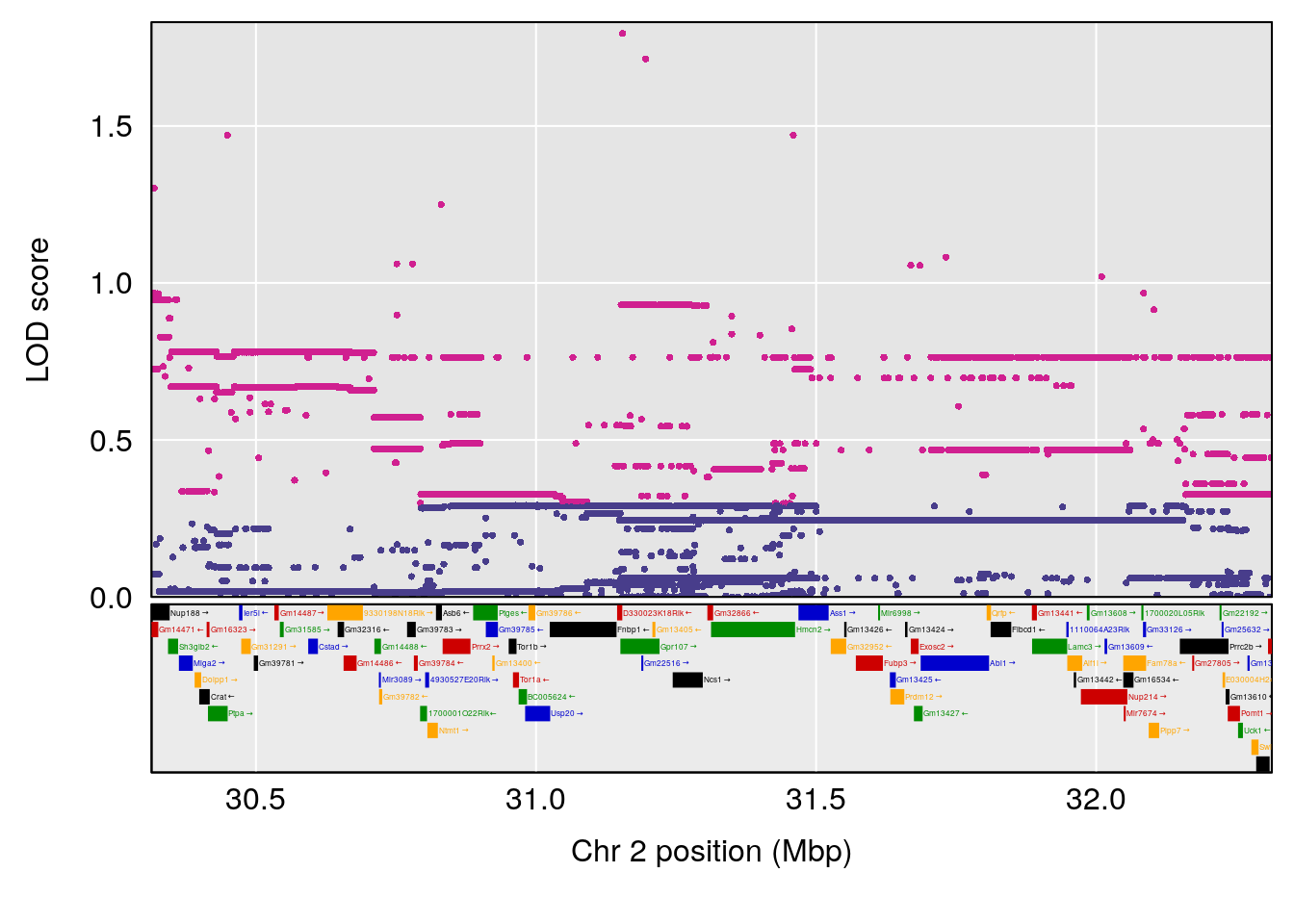
# [1] 2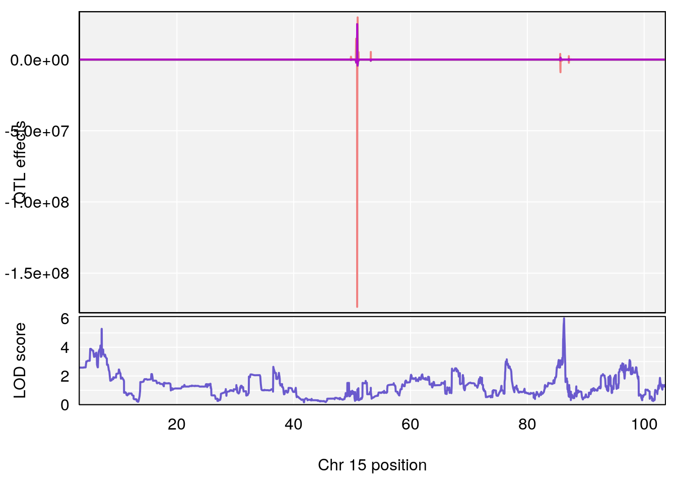
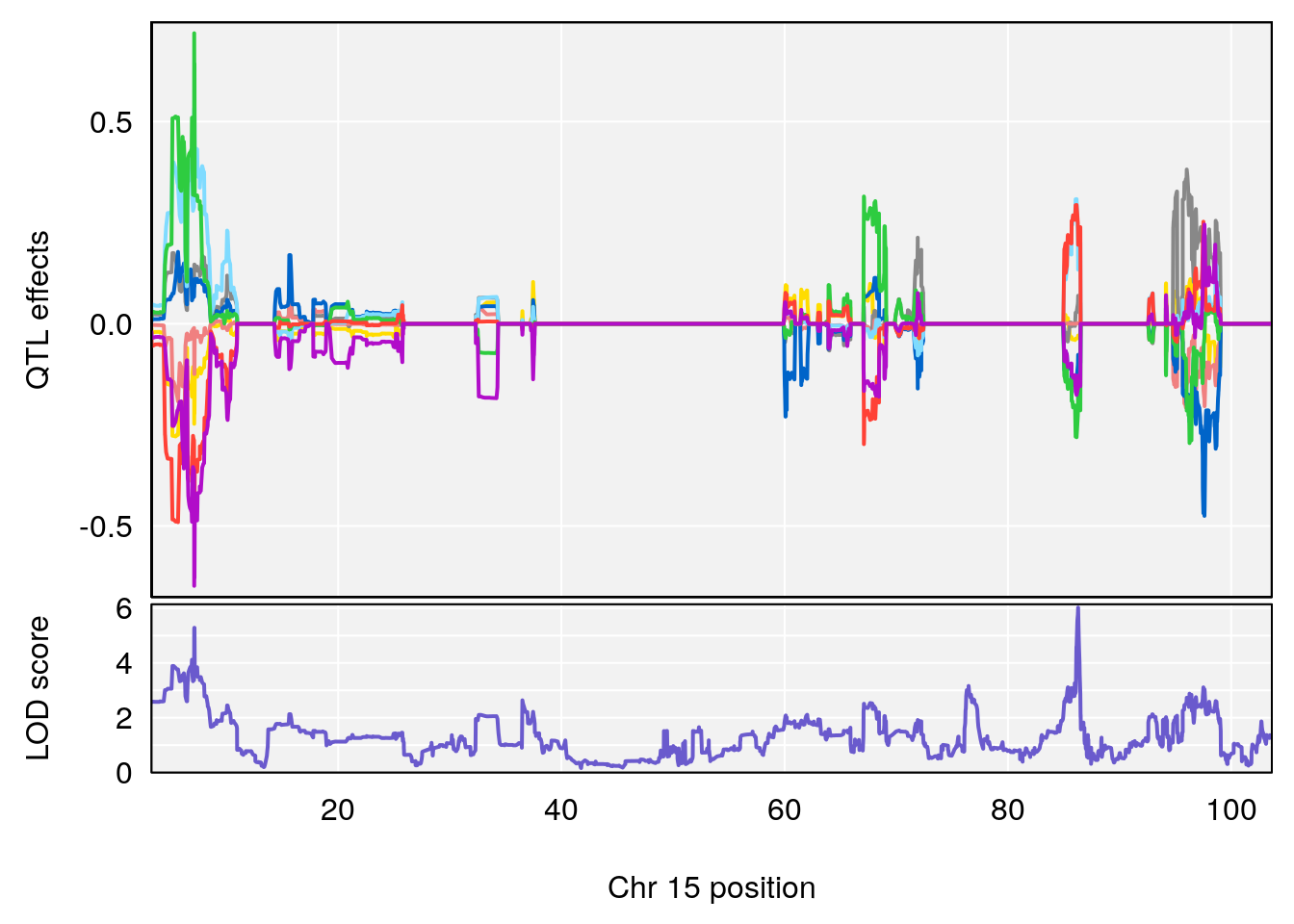
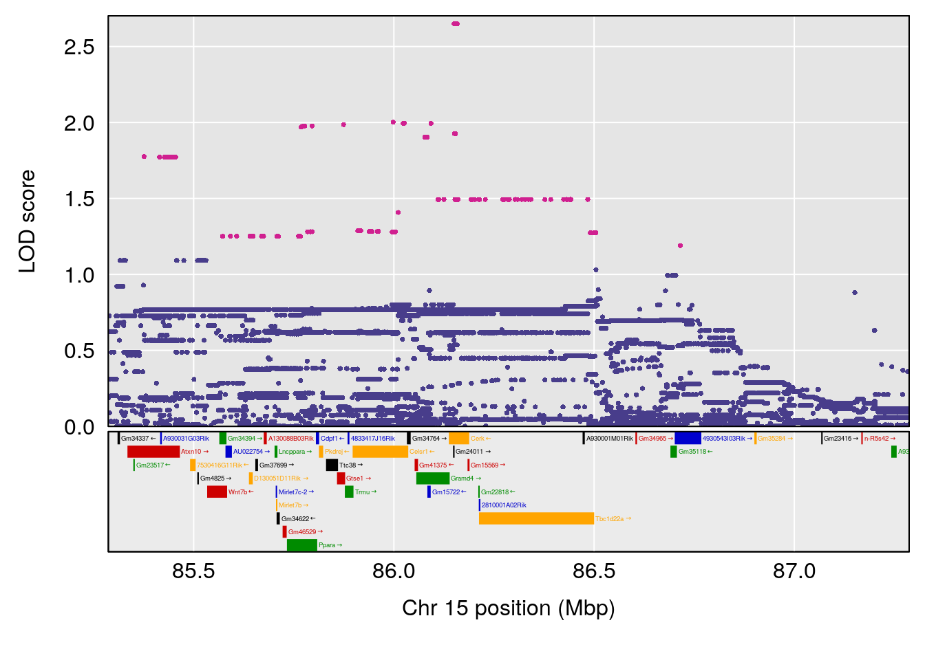
# [1] "EIP__ms"
#   lodindex lodcolumn chr      pos      lod    ci_lo     ci_hi
# 1        1    pheno1  10 56.54059 6.010974 53.99479 123.43250
# 2        1    pheno1  15 43.77368 6.307630 42.28269  50.39496
# [1] 1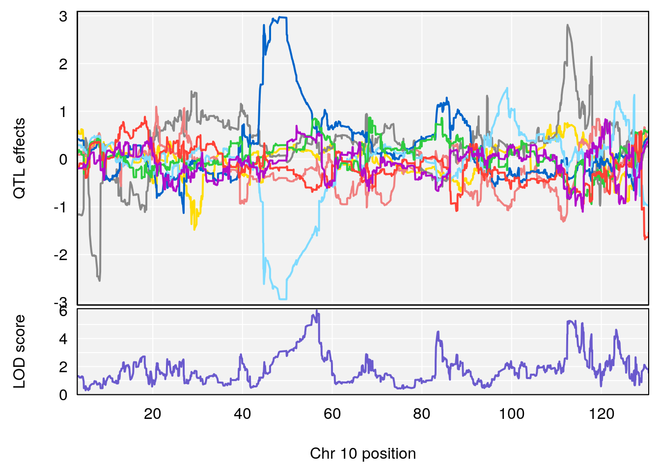
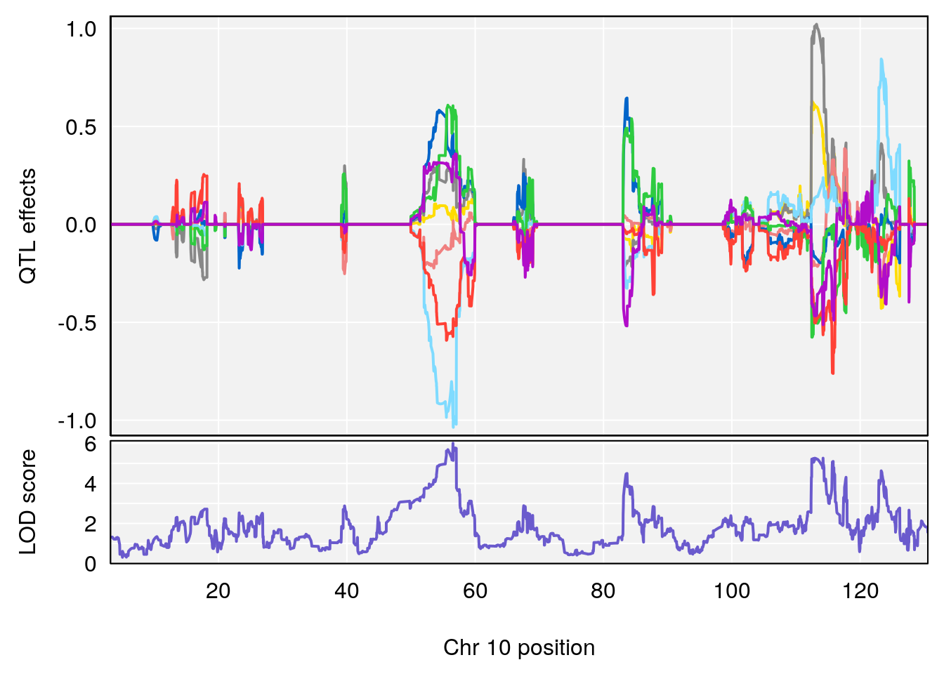
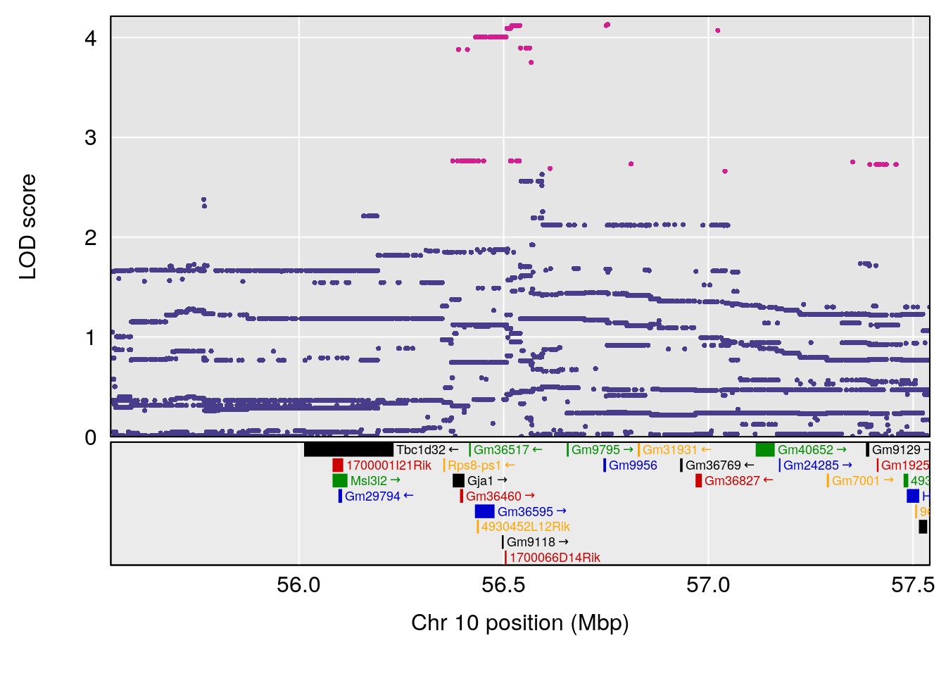
# [1] 2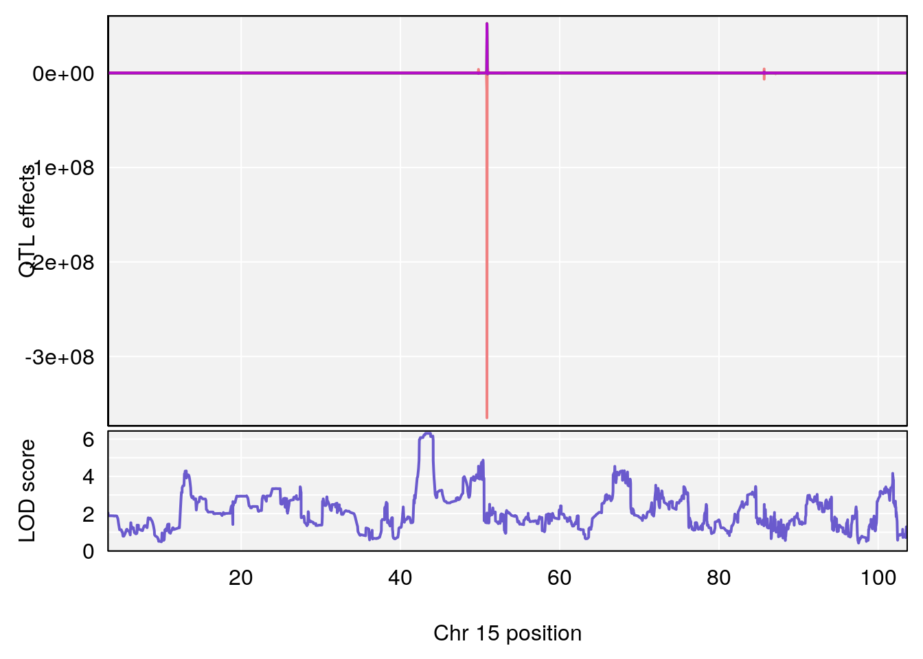
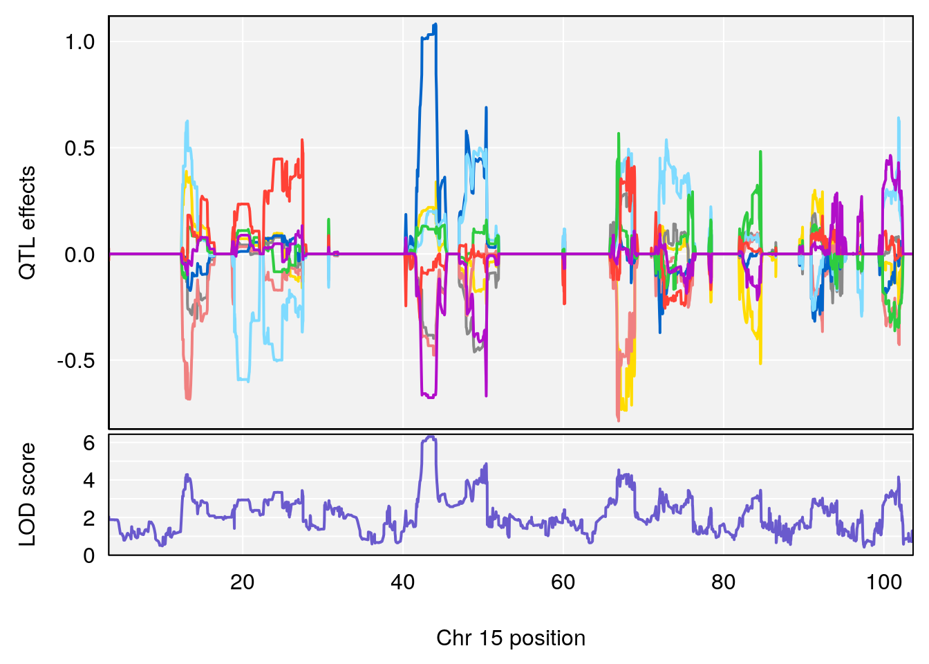
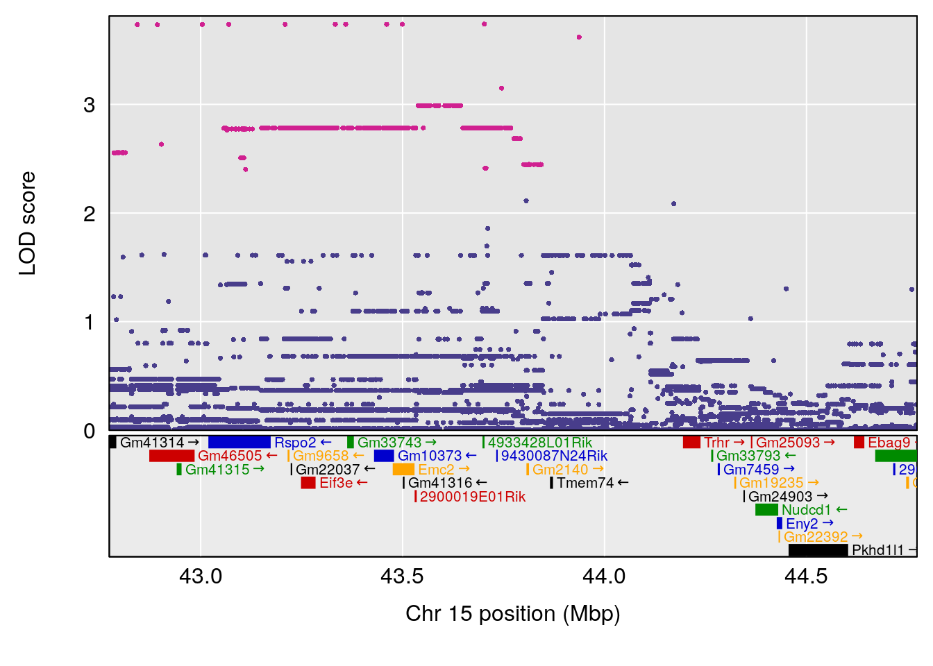
# [1] "EEP_9ms"
#   lodindex lodcolumn chr      pos      lod    ci_lo    ci_hi
# 1        1    pheno1  15 97.45622 7.546755 97.15079 97.69967
# 2        1    pheno1  19 35.75904 6.048214 31.82253 36.17606
# [1] 1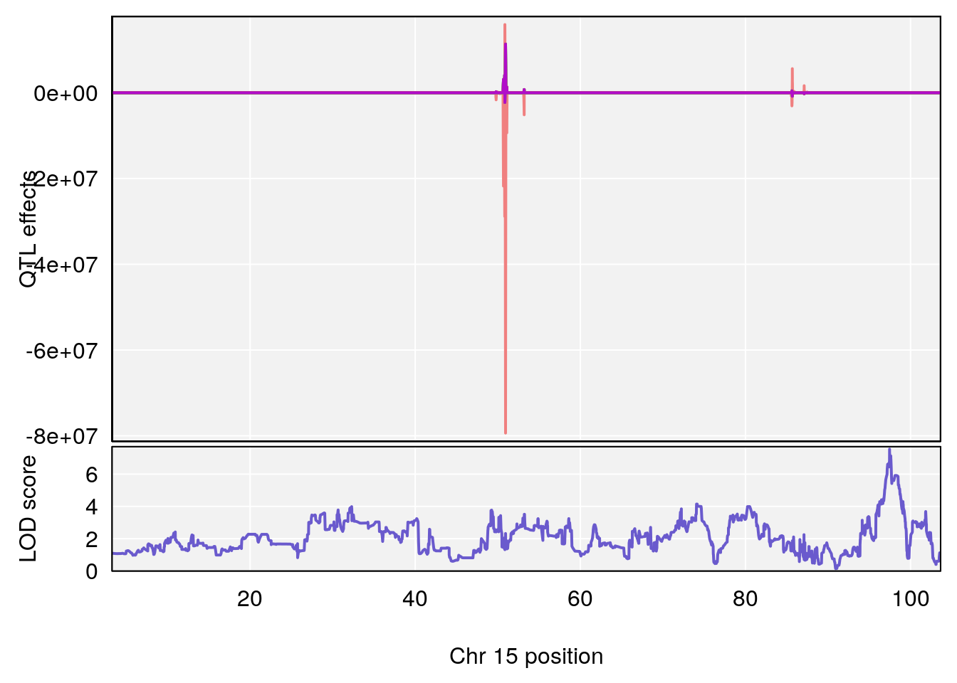
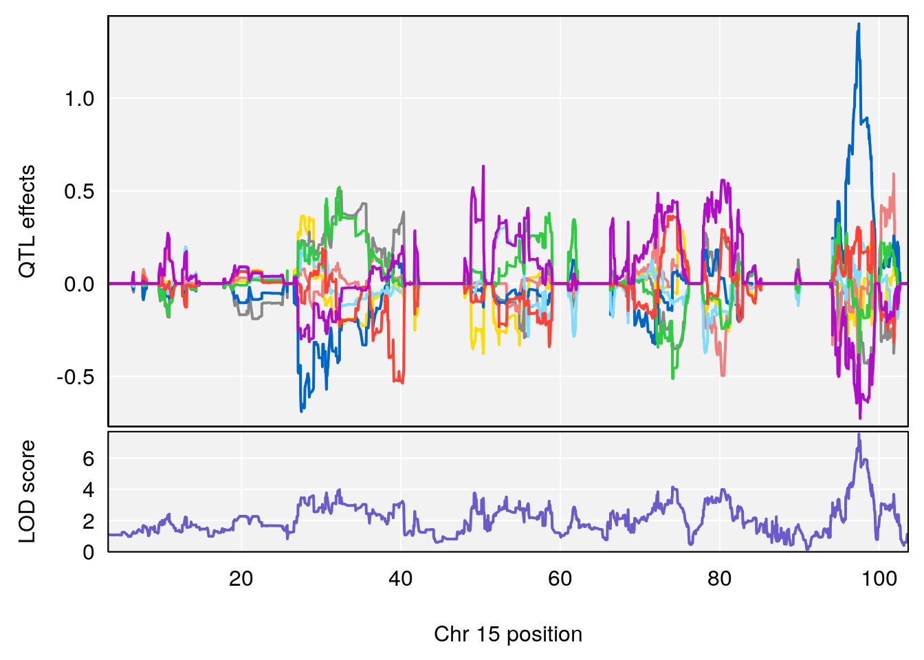
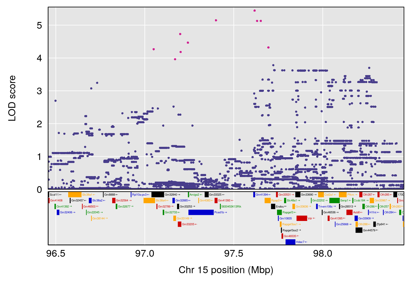
# [1] 2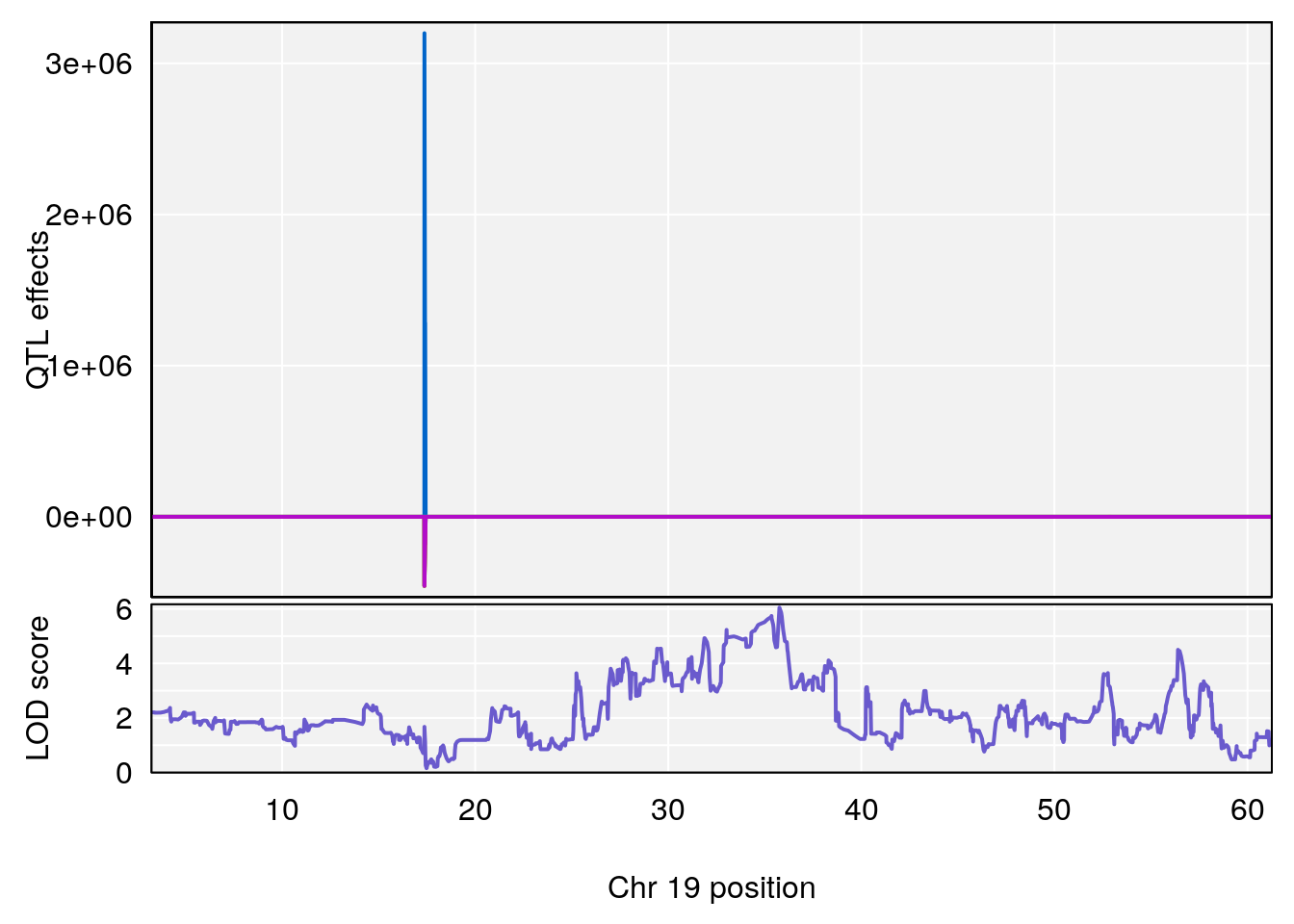
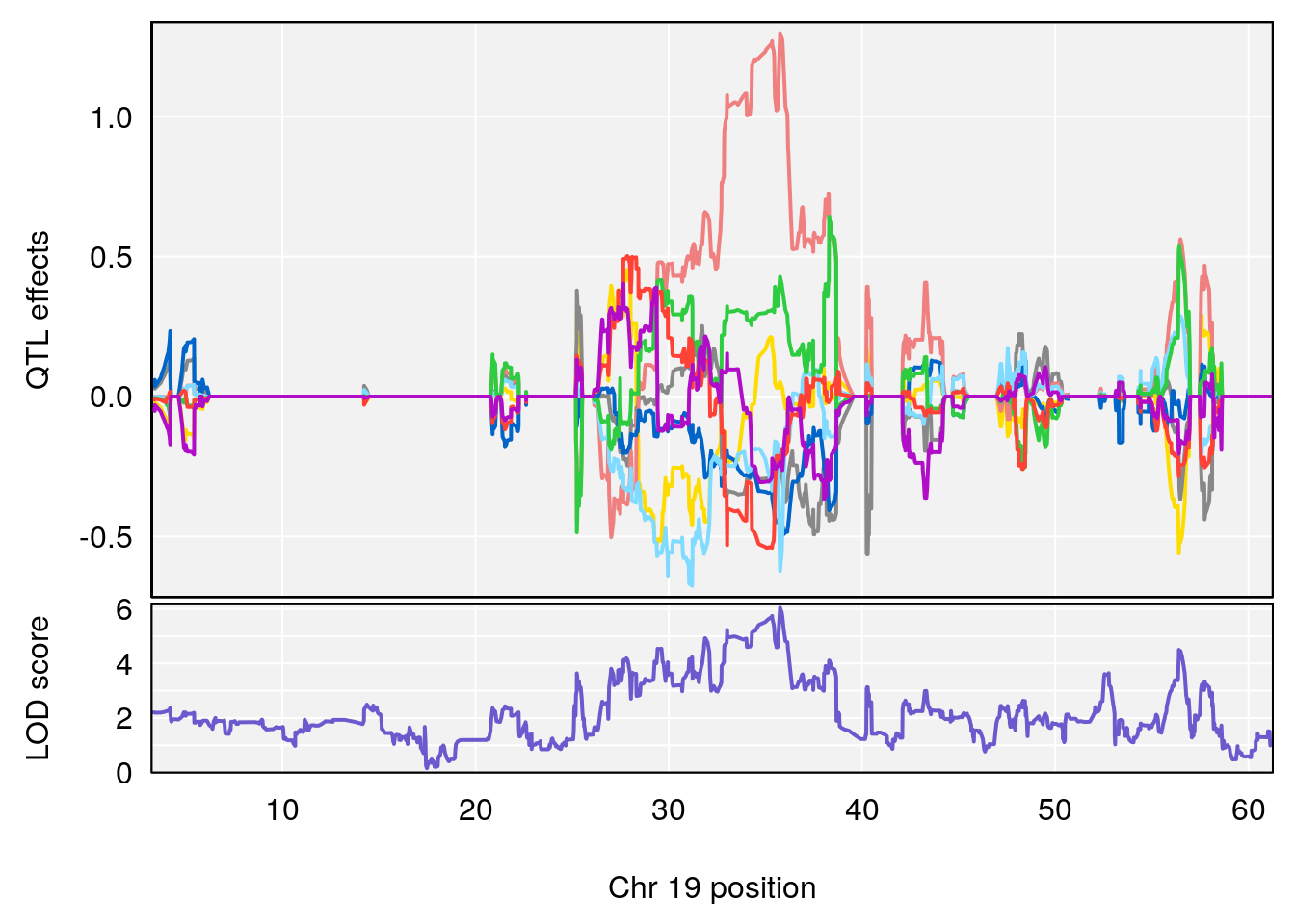
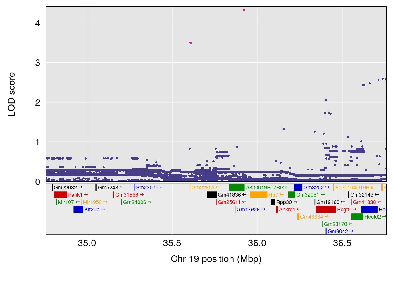
# [1] "Tr__sec"
# [1] lodindex  lodcolumn chr       pos       lod       ci_lo     ci_hi
# <0 rows> (or 0-length row.names)
# [1] "TB"
#   lodindex lodcolumn chr      pos      lod    ci_lo    ci_hi
# 1        1    pheno1  14 105.5591 6.078798 20.32646 108.1971
# [1] 1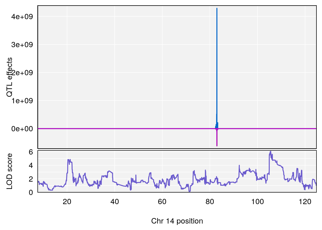
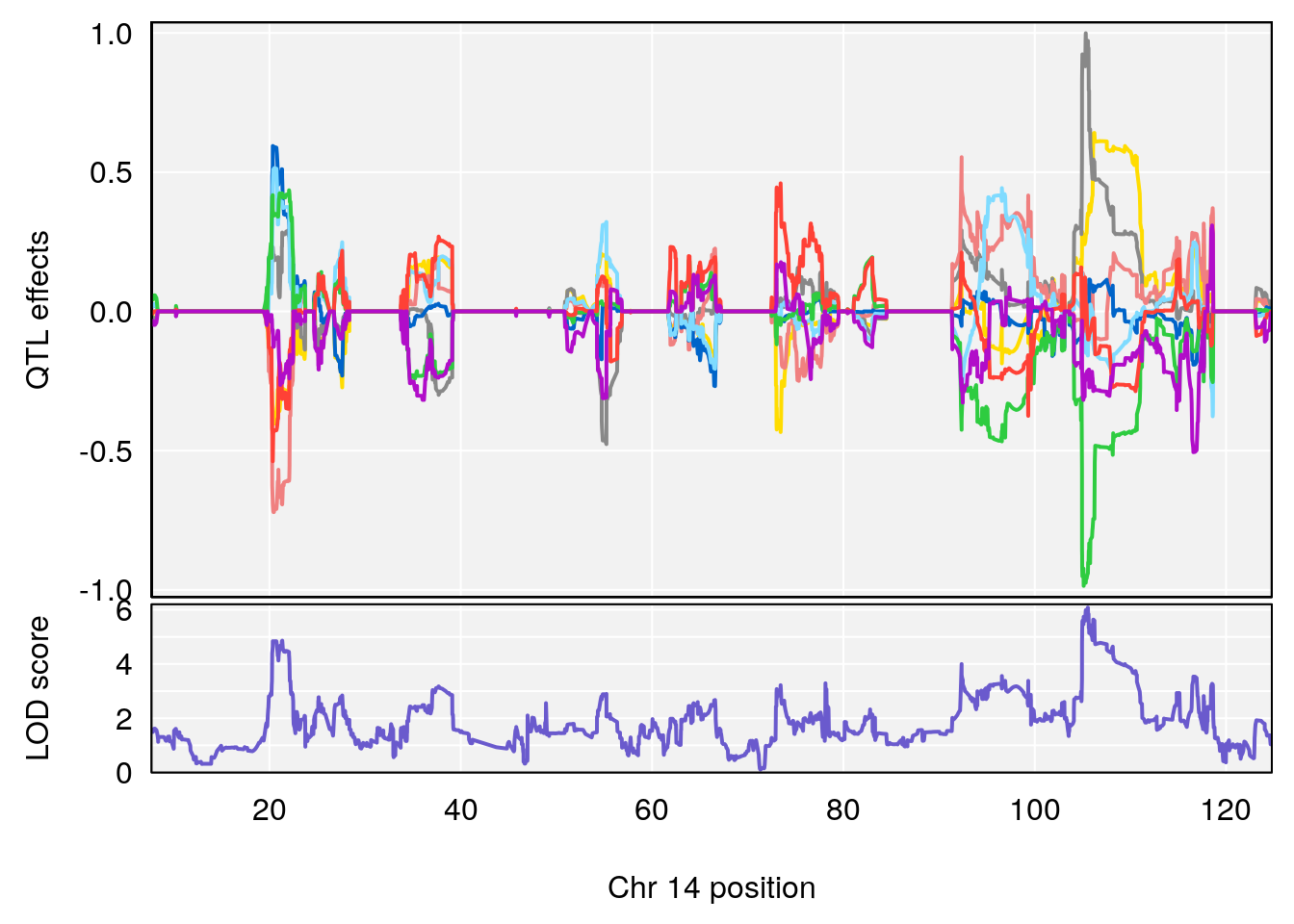
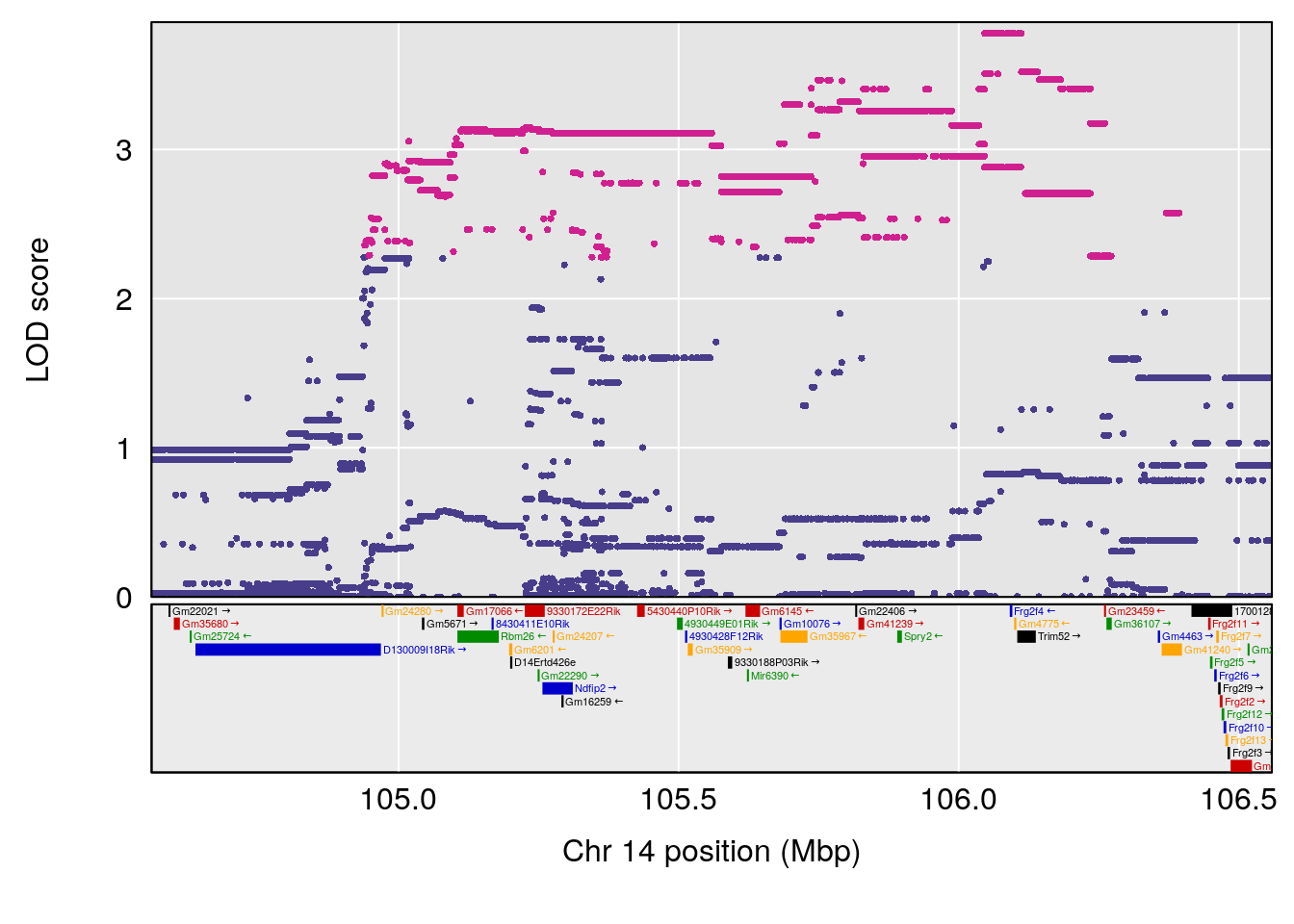
# [1] "TP"
#   lodindex lodcolumn chr      pos      lod    ci_lo    ci_hi
# 1        1    pheno1   3 18.88115 6.125924 17.06440 19.72964
# 2        1    pheno1  11 45.34345 6.588552 43.47646 45.50121
# 3        1    pheno1  12 34.88396 6.055593 34.82905 36.07517
# [1] 1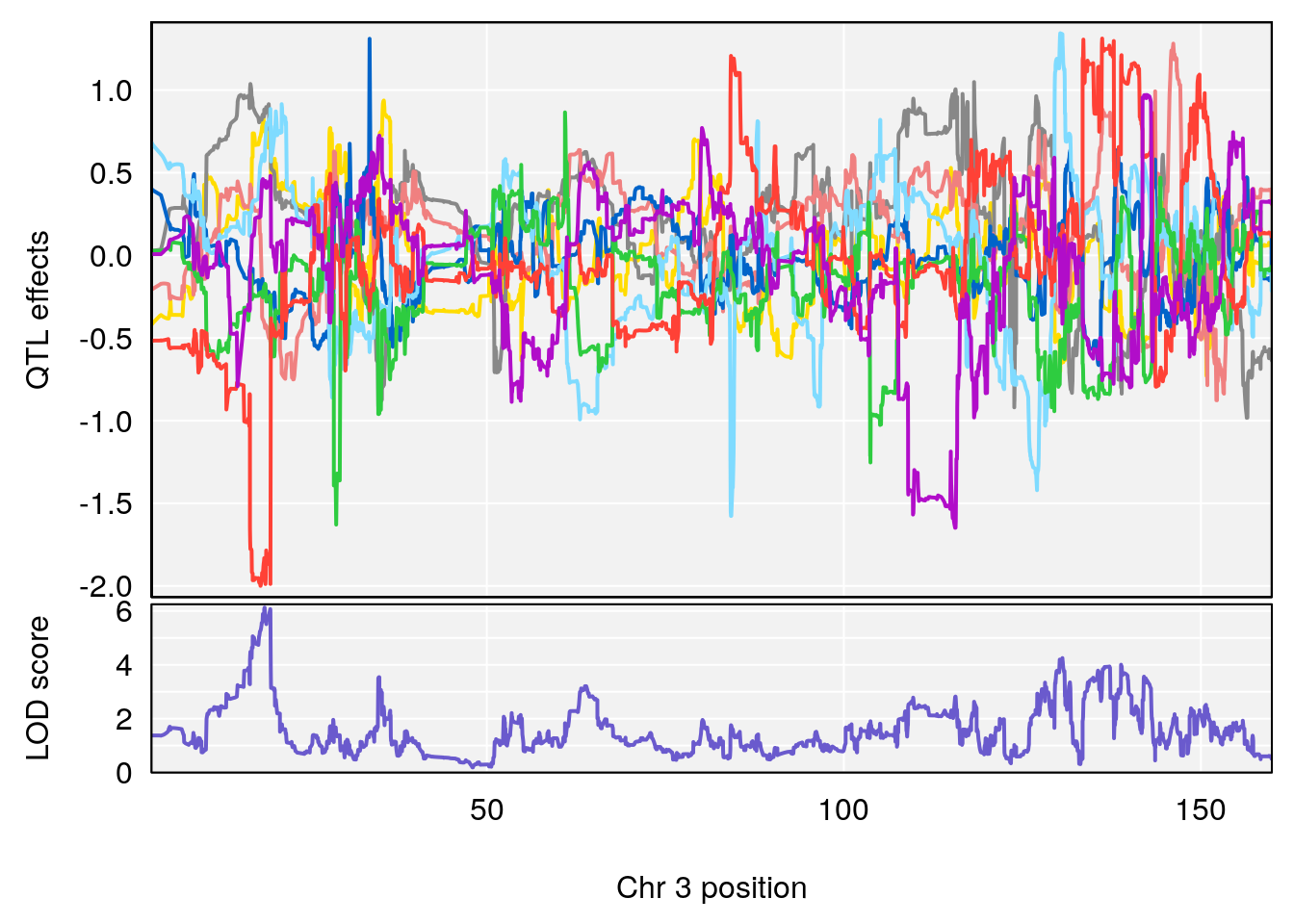
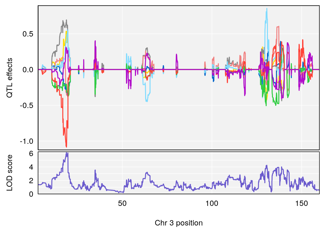
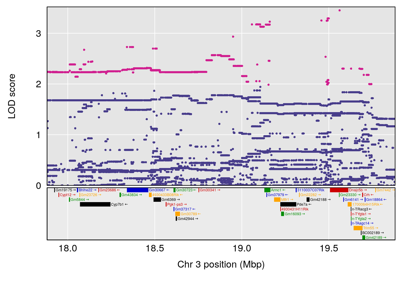
# [1] 2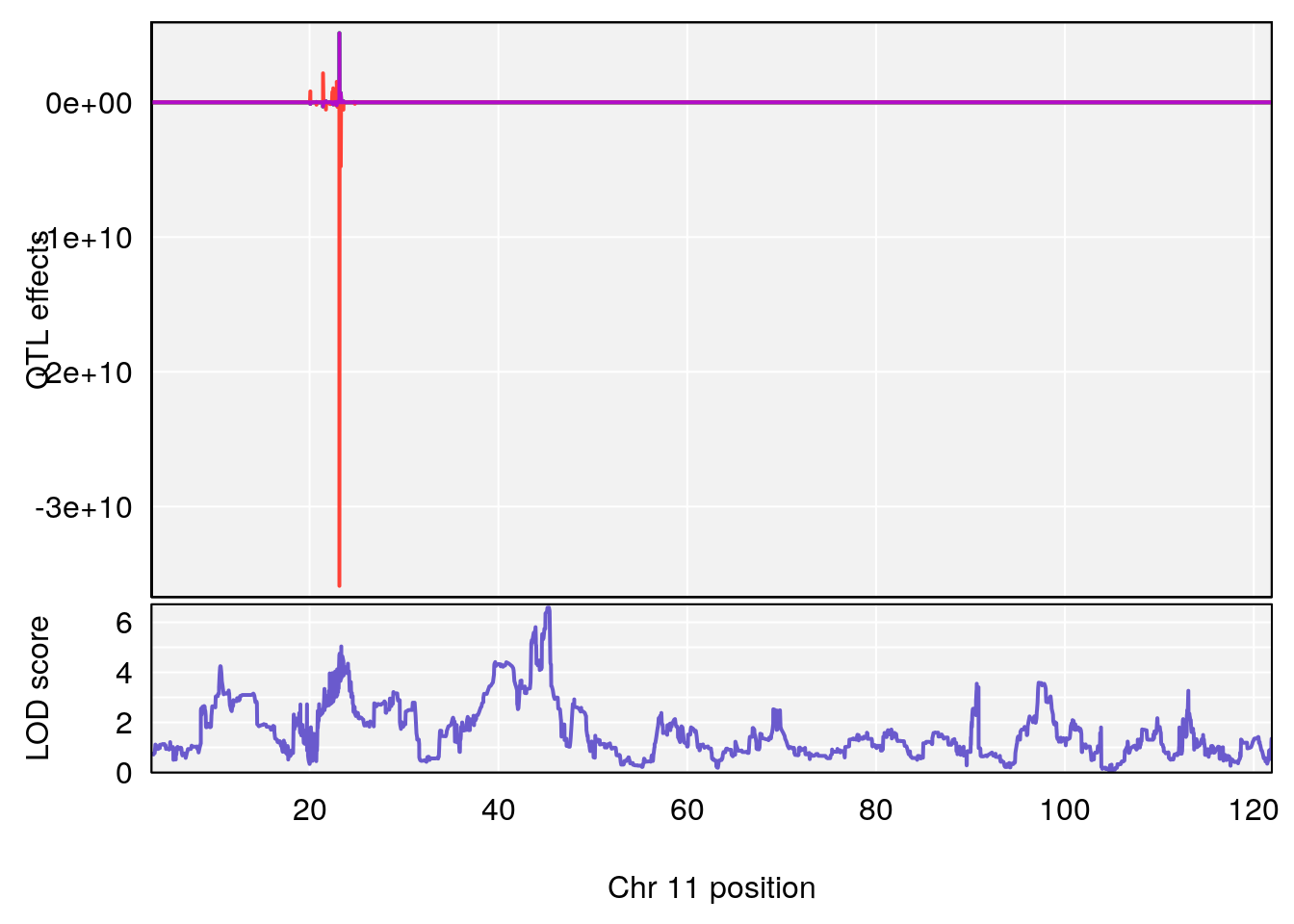
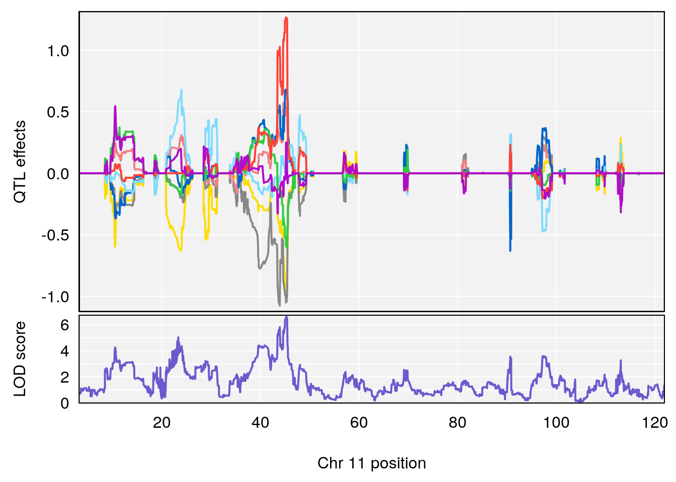
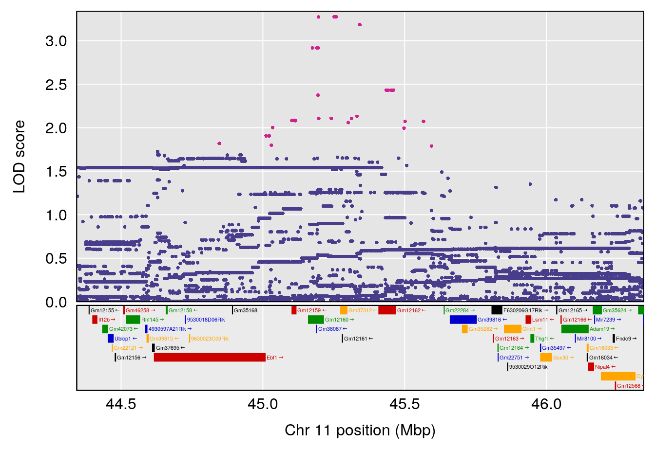
# [1] 3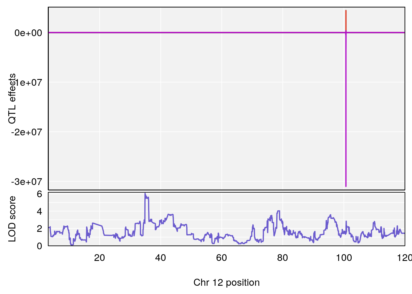
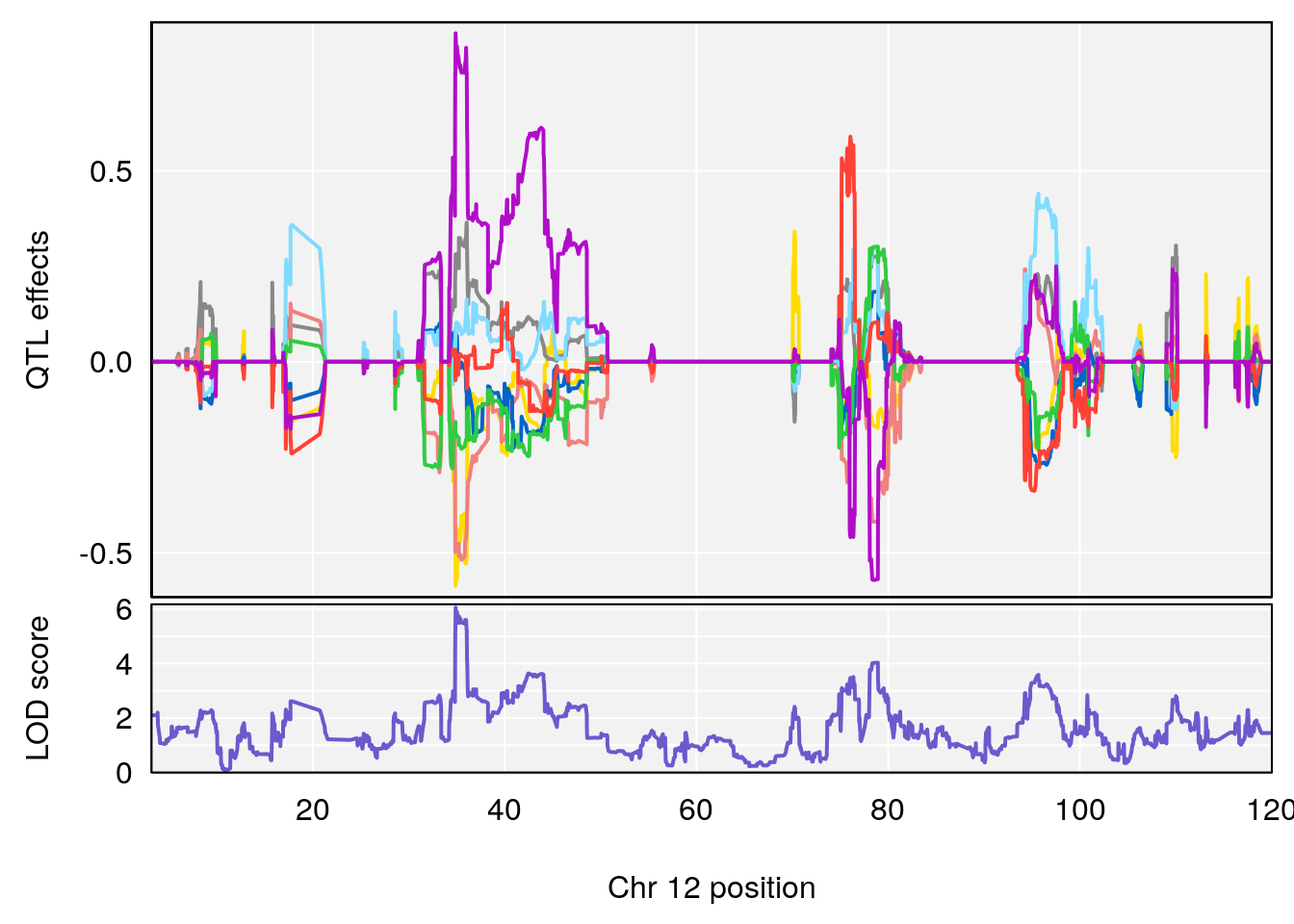
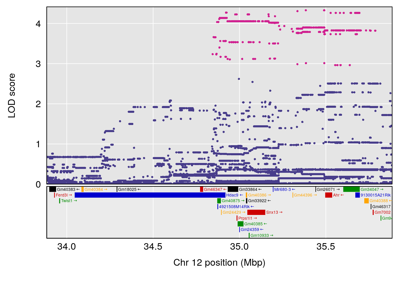
# [1] "Rinx"
#   lodindex lodcolumn chr      pos      lod     ci_lo    ci_hi
# 1        1    pheno1   1 133.1683 6.333351 35.878973 150.4046
# 2        1    pheno1   5 130.3330 6.315787  3.043534 135.8304
# 3        1    pheno1  14 105.5591 6.202362 21.022237 108.2466
# [1] 1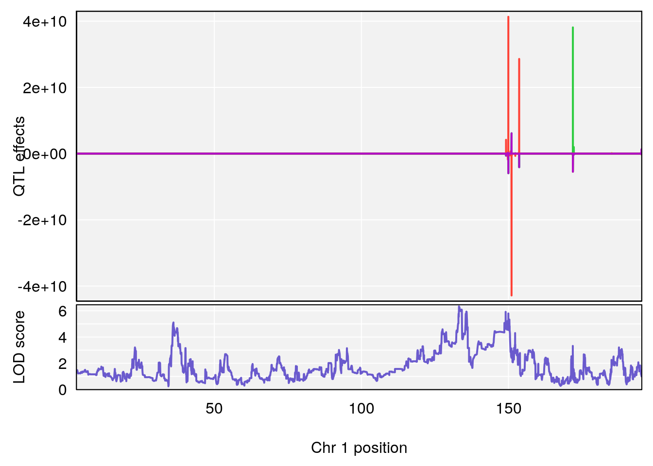
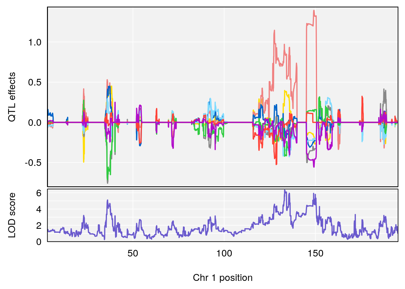
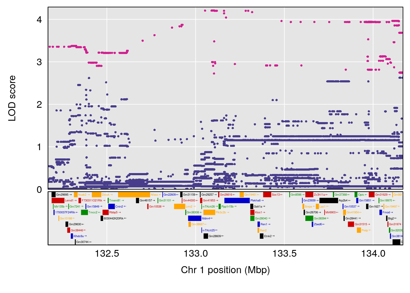
# [1] 2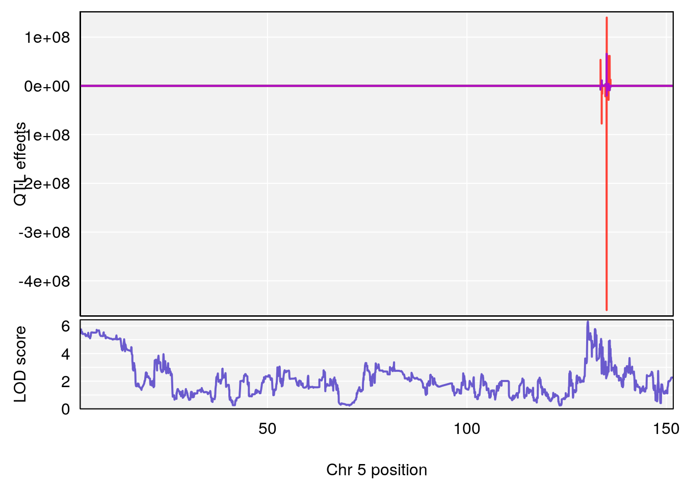
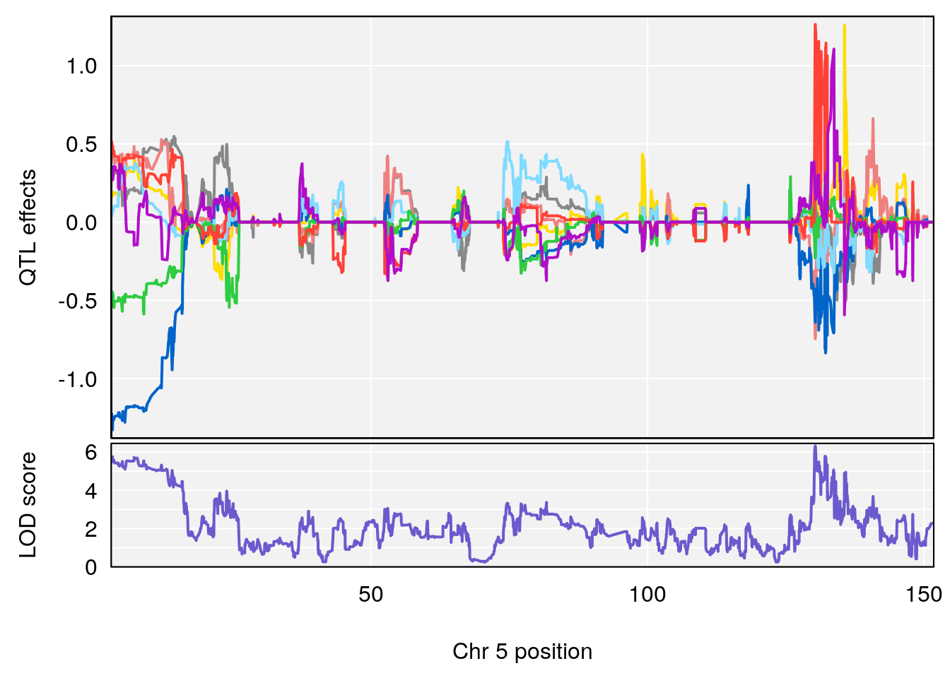
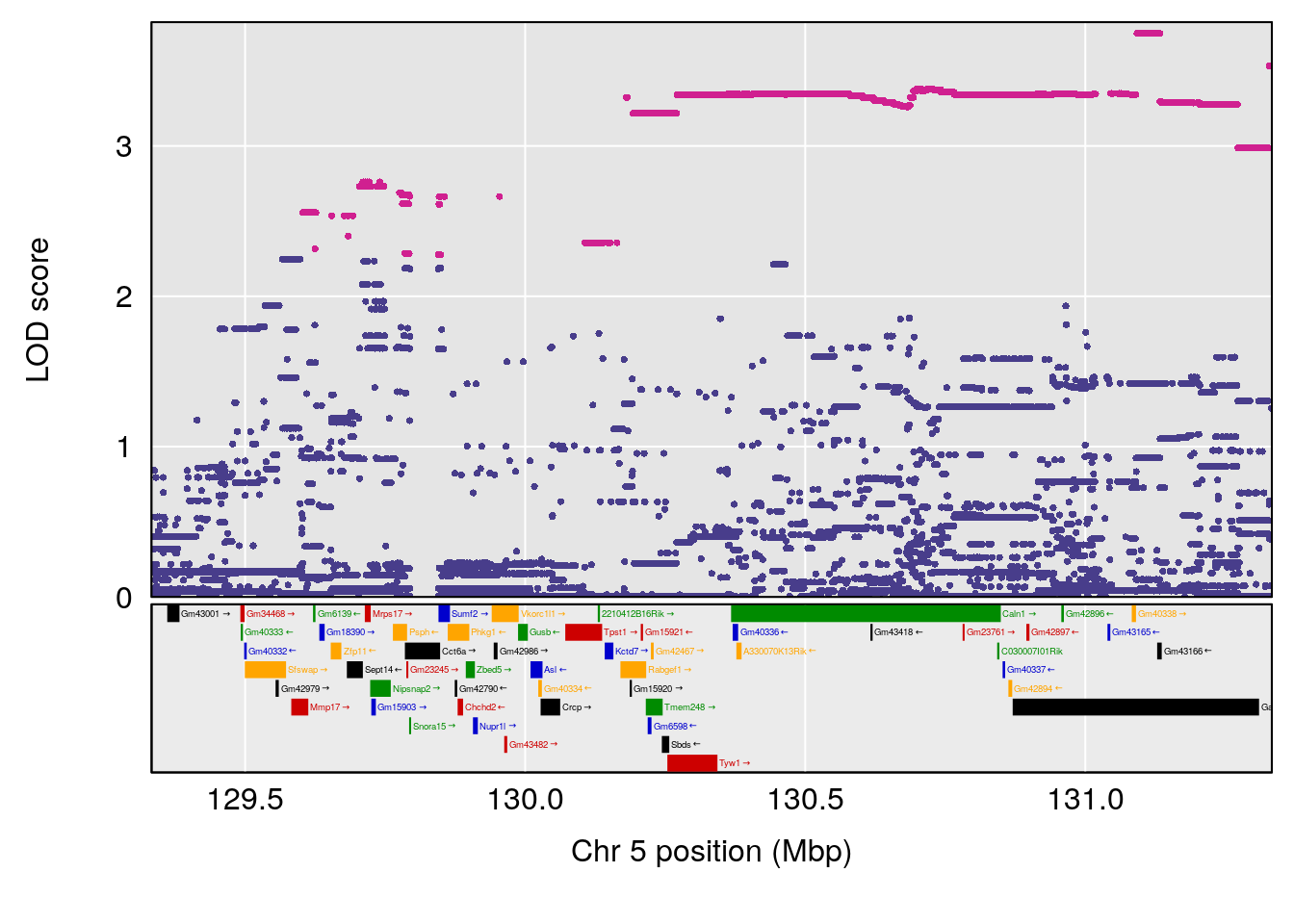
# [1] 3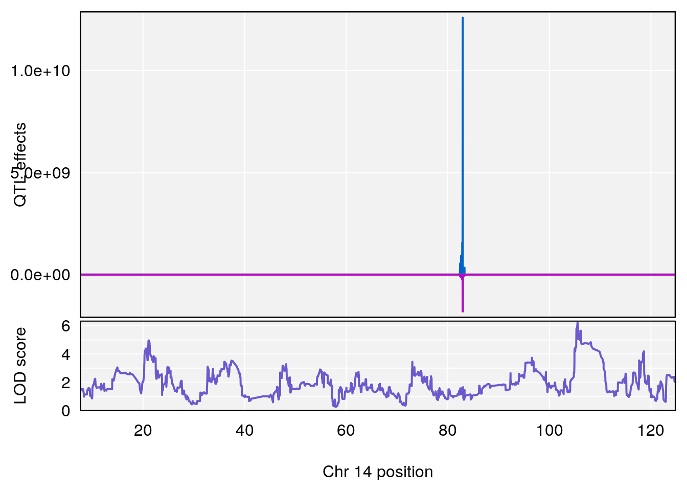
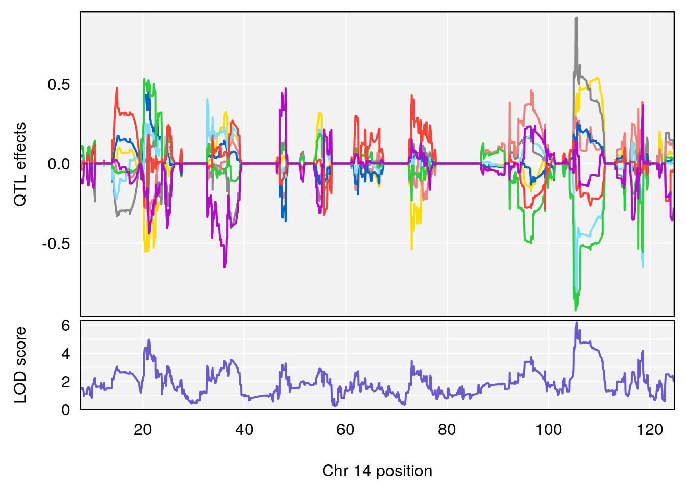
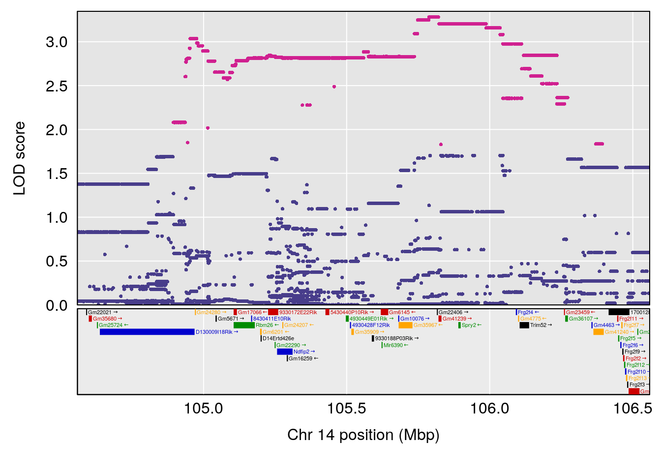
# [1] "Ttot"
#   lodindex lodcolumn chr       pos      lod     ci_lo    ci_hi
# 1        1    pheno1   1 149.95860 6.071108 127.23477 150.5381
# 2        1    pheno1   X  97.36966 6.109065  97.27061 100.6561
# [1] 1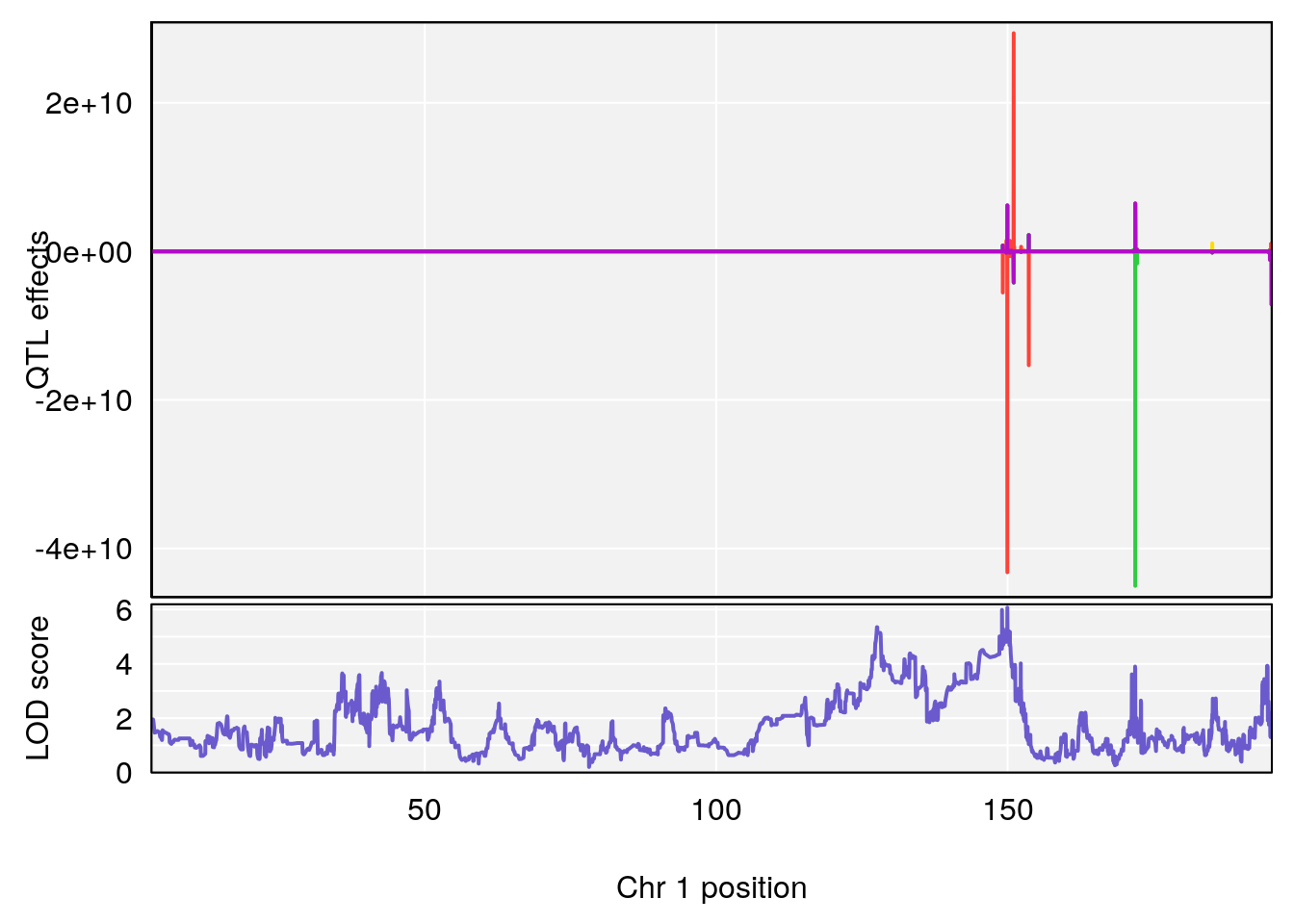
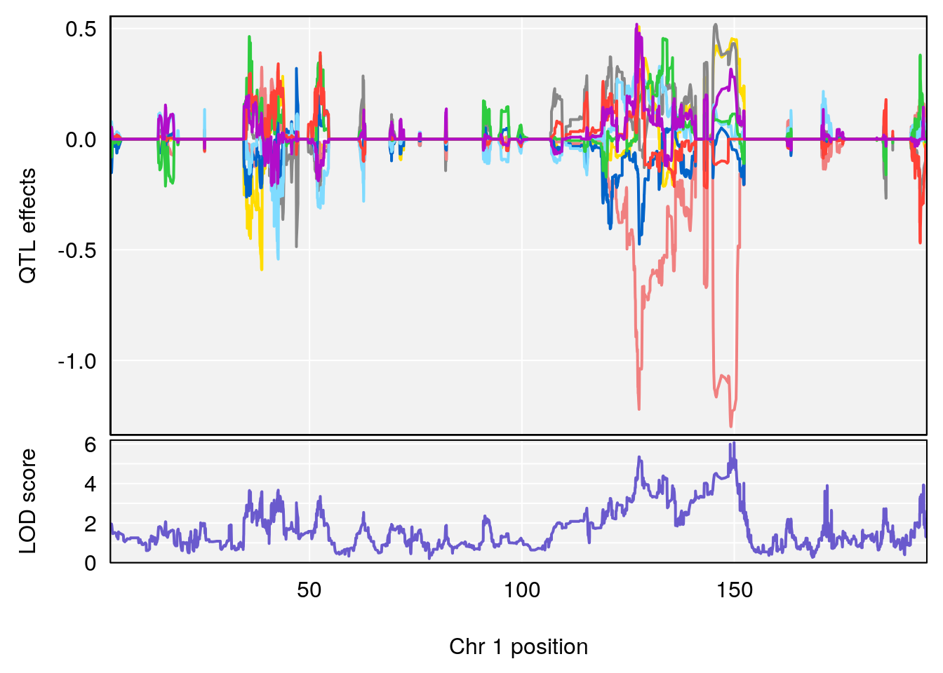
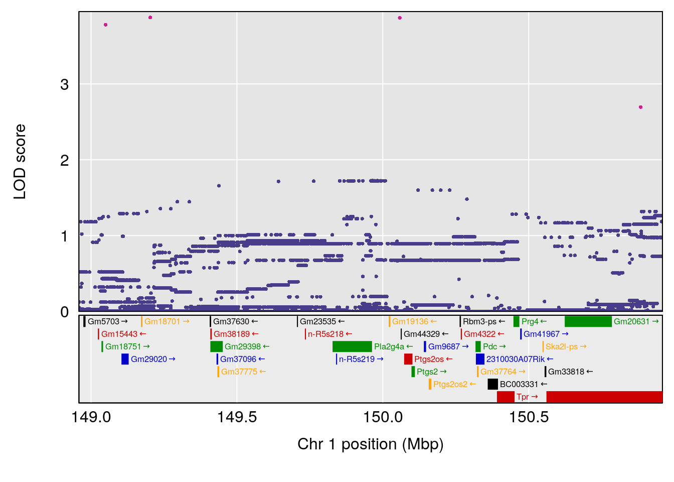
# [1] 2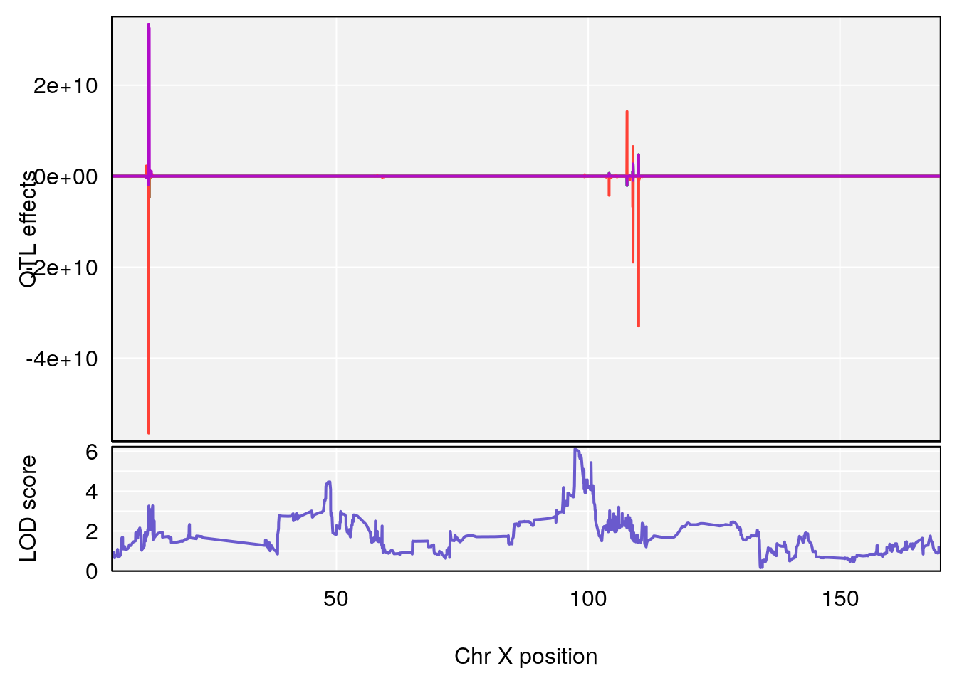
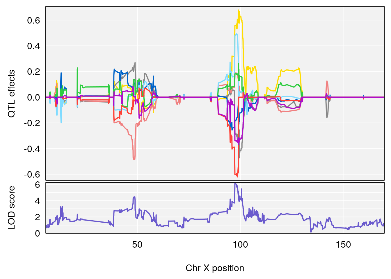
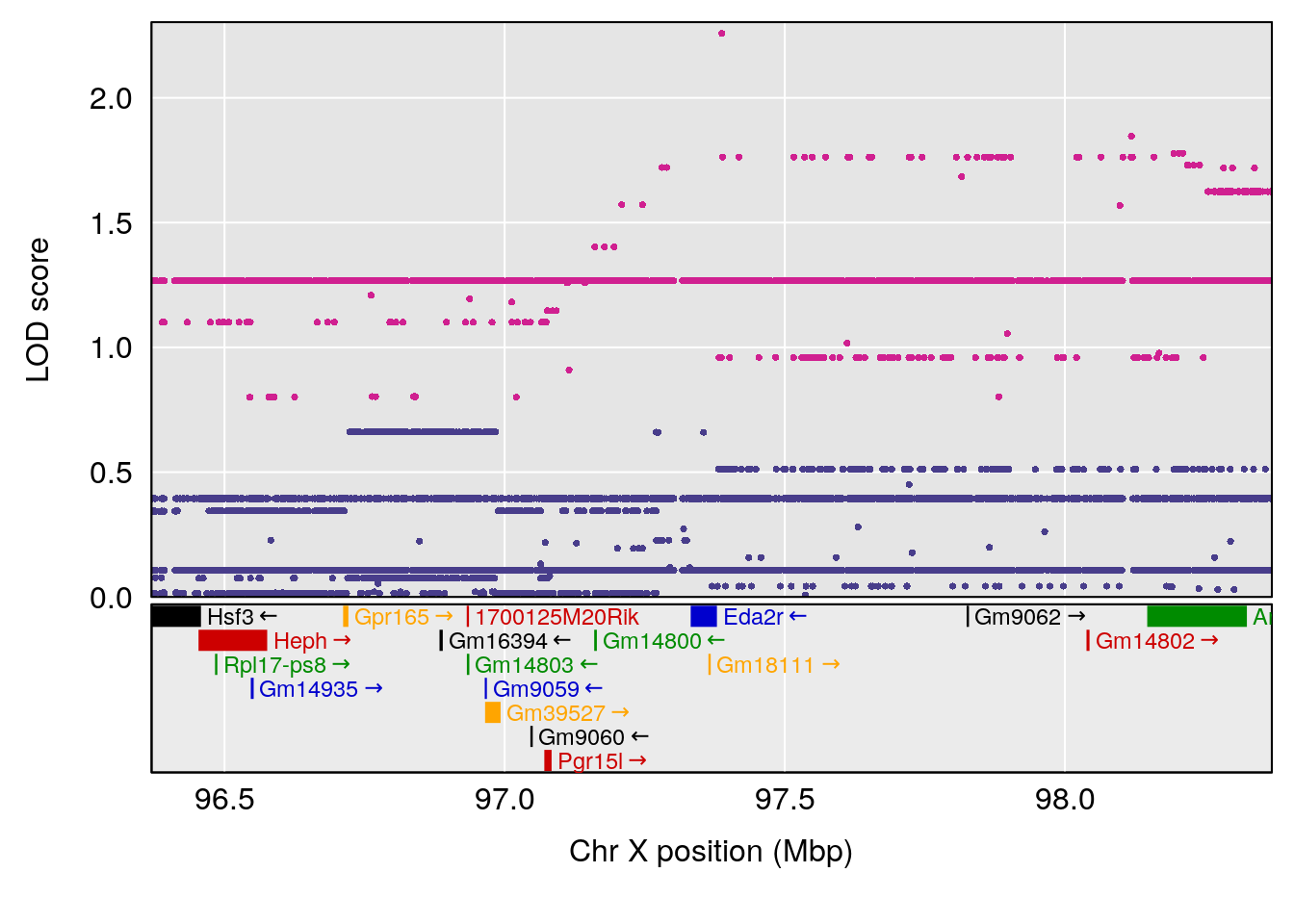
# [1] "duty_cycle"
# [1] lodindex  lodcolumn chr       pos       lod       ci_lo     ci_hi
# <0 rows> (or 0-length row.names)
# [1] "resp_flow"
#   lodindex lodcolumn chr      pos      lod    ci_lo    ci_hi
# 1        1    pheno1   2 31.31643 6.731936 30.97043 32.48273
# [1] 1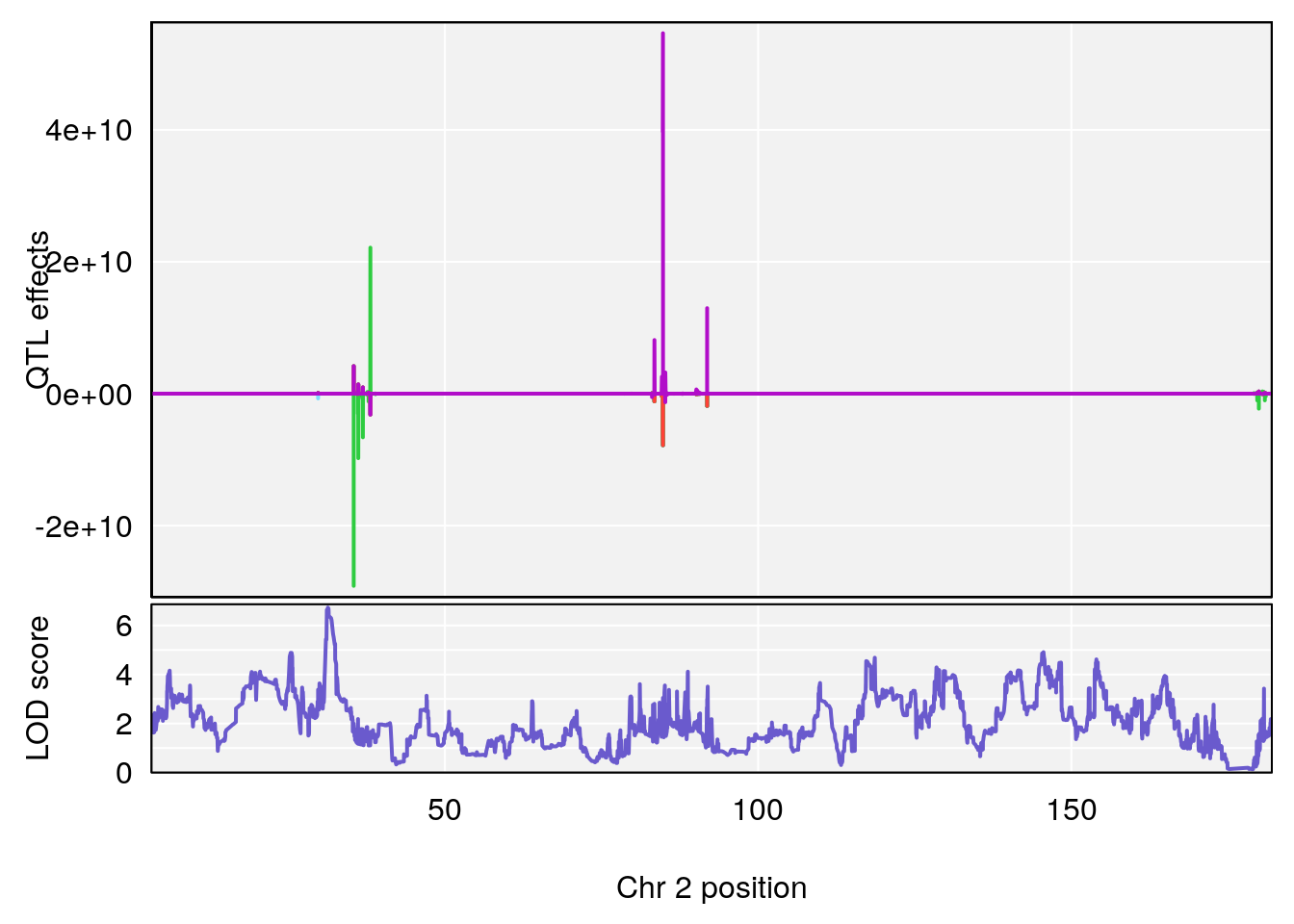
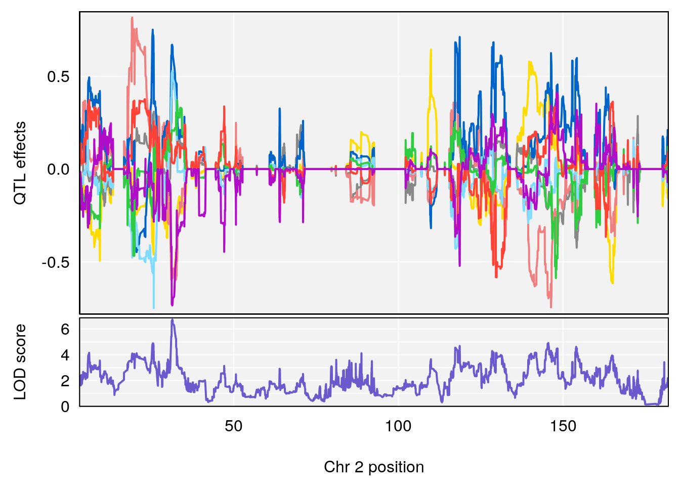
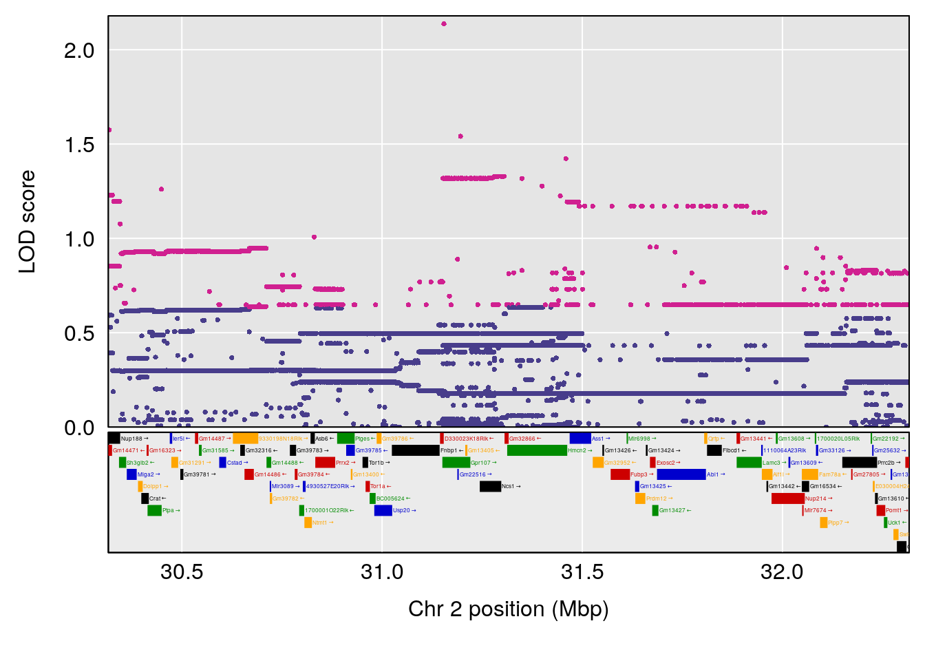
# [1] "insp_flow"
#   lodindex lodcolumn chr      pos      lod    ci_lo    ci_hi
# 1        1    pheno1   2 31.37817 6.759318 30.89733 32.48273
# [1] 1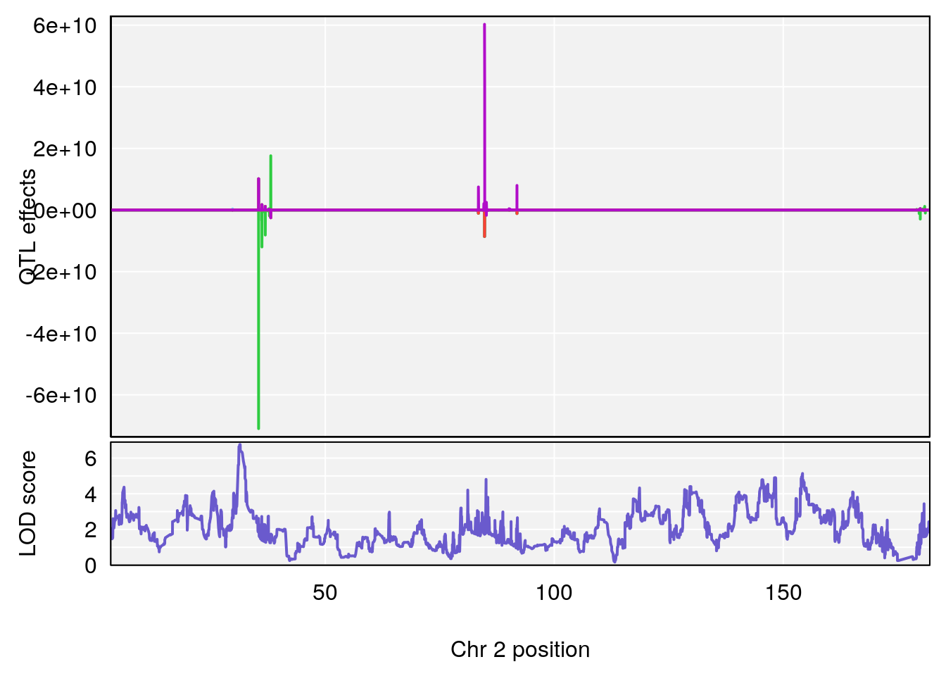
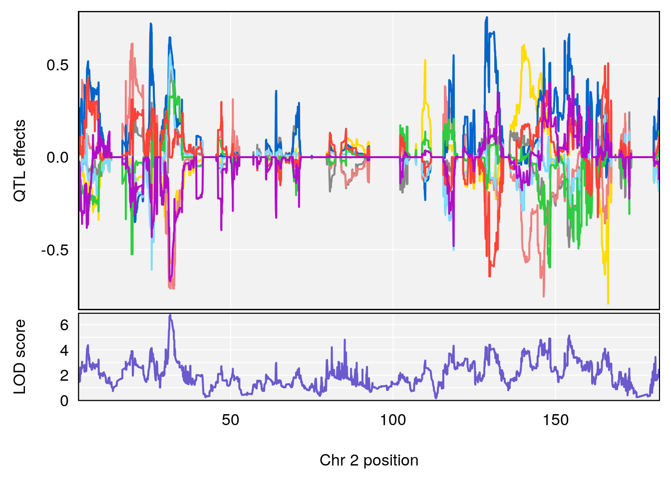
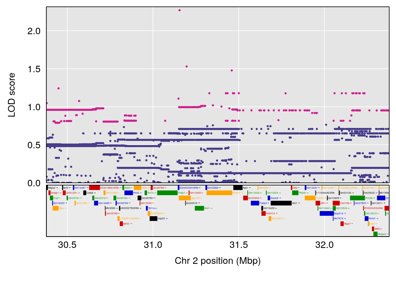
# [1] "exp_flow"
#   lodindex lodcolumn chr      pos      lod    ci_lo   ci_hi
# 1        1    pheno1   2 31.31643 6.475736 25.22602 117.387
# [1] 1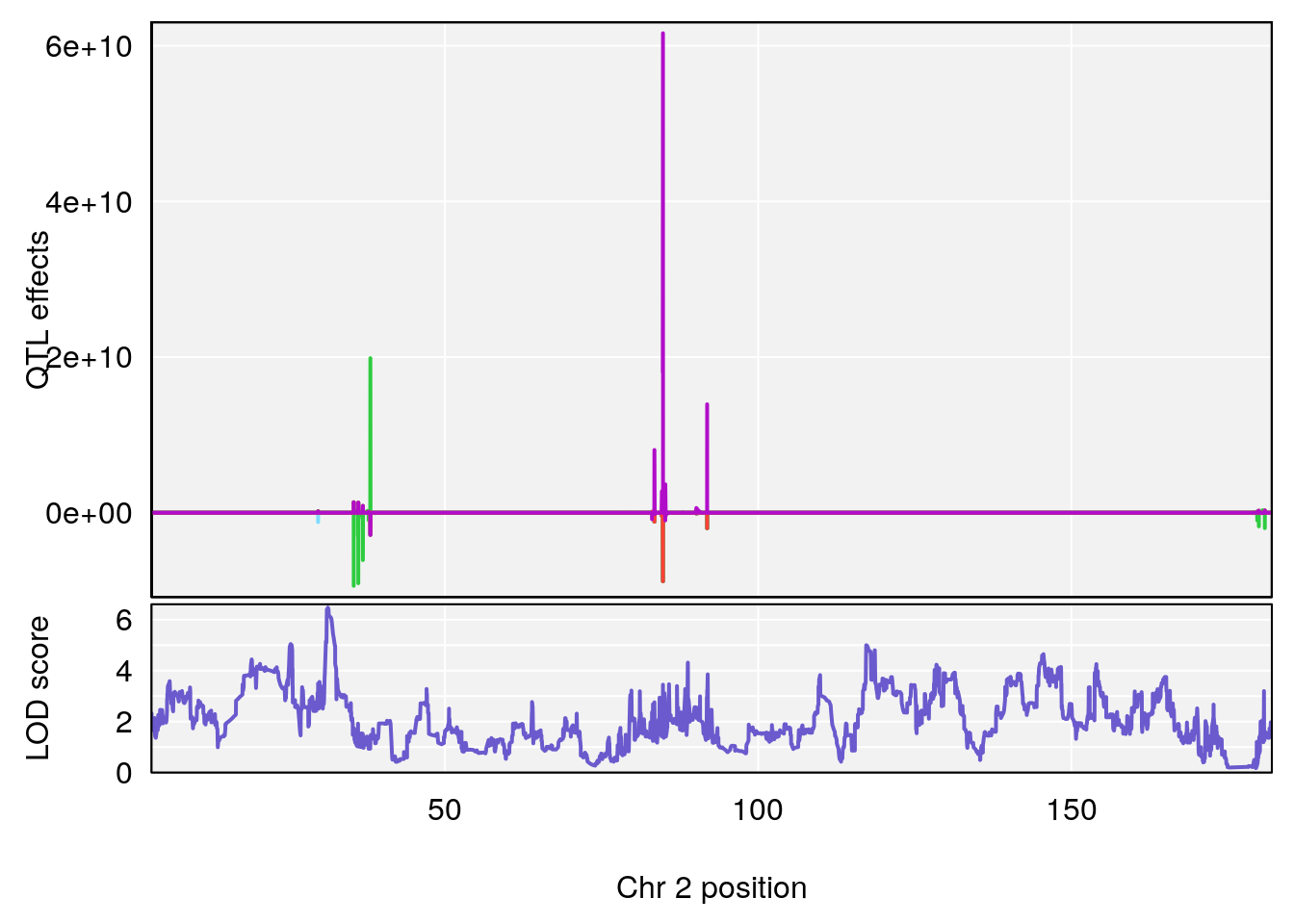
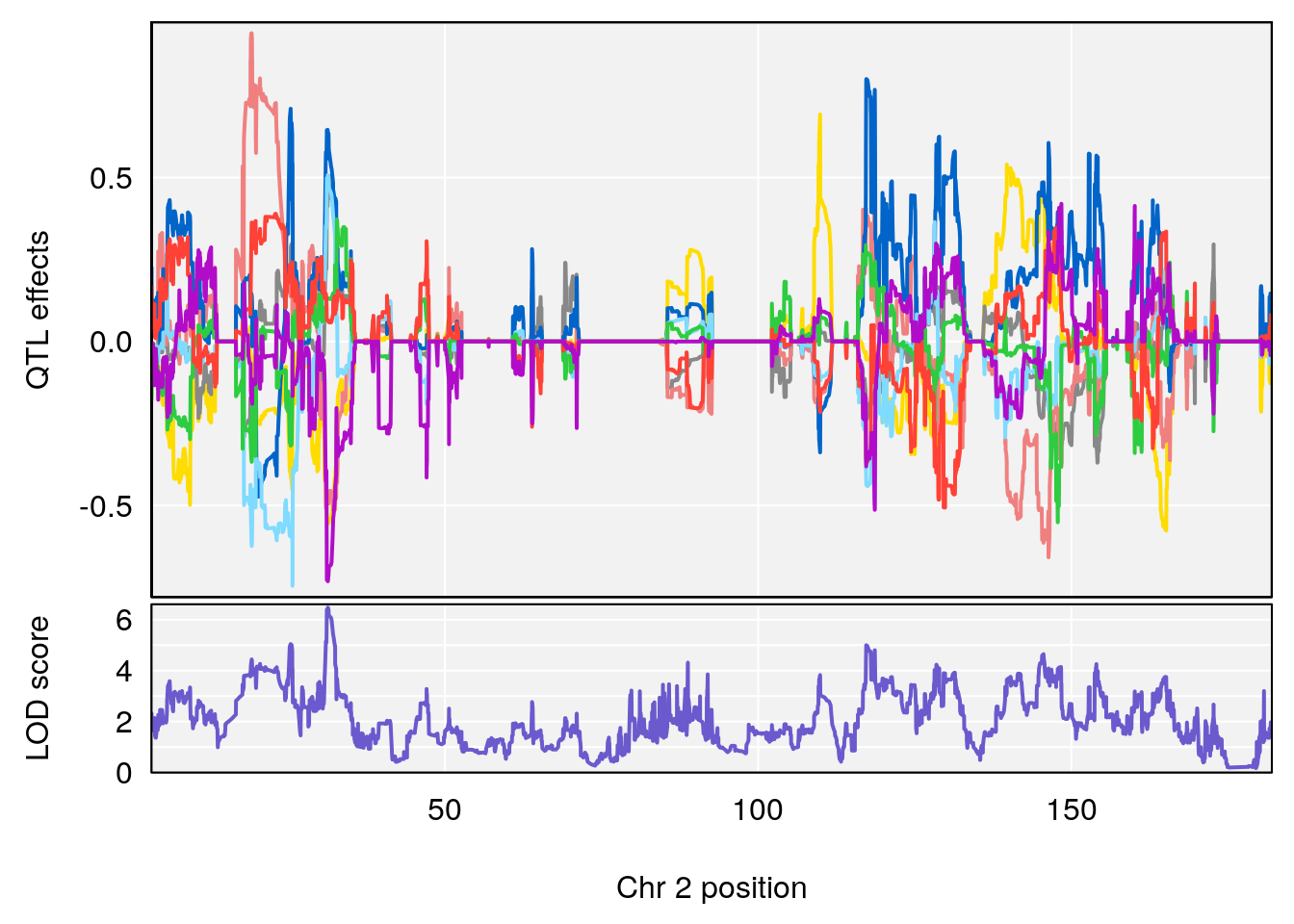
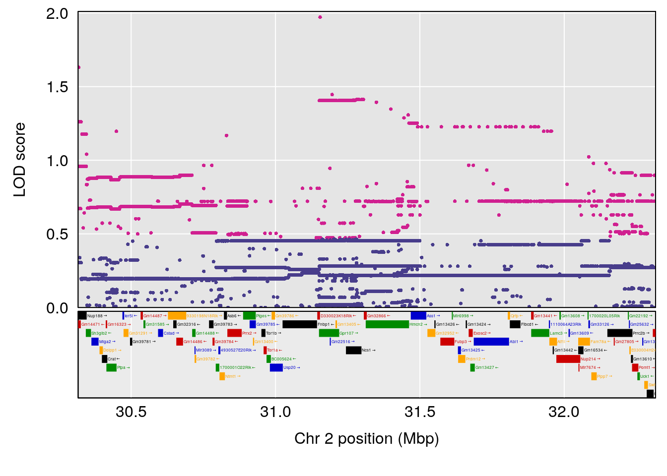
Plot qtl mapping on array female
load("output/Fentanyl/qtl.fentanyl.out.female.RData")

#genome-wide plot
for(i in names(qtl.morphine.out)){
  par(mar=c(5.1, 4.1, 1.1, 1.1))
  ymx <- maxlod(qtl.morphine.out[[i]]) # overall maximum LOD score
  plot(qtl.morphine.out[[i]], map=gm$pmap, lodcolumn=1, col="slateblue", ylim=c(0, max(sapply(qtl.morphine.out, maxlod)) +2))
  abline(h=summary(qtl.morphine.operm[[i]], alpha=c(0.10, 0.05, 0.01))[[1]], col="red")
  abline(h=summary(qtl.morphine.operm[[i]], alpha=c(0.10, 0.05, 0.01))[[2]], col="red")
  abline(h=summary(qtl.morphine.operm[[i]], alpha=c(0.10, 0.05, 0.01))[[3]], col="red")
  title(main = paste0("DO_fentanyl_",i))
}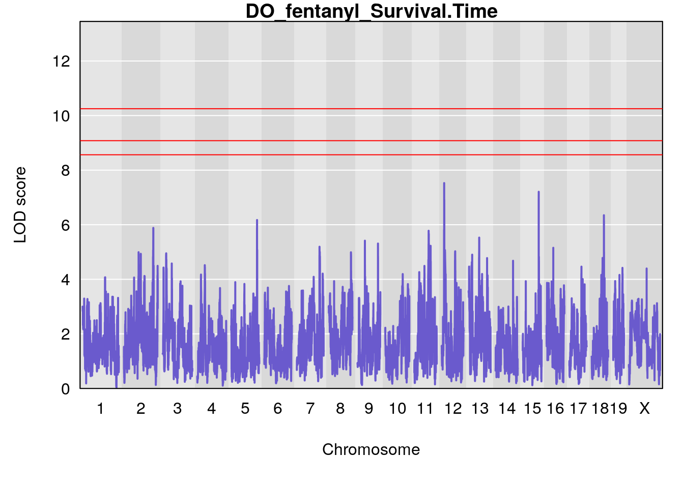
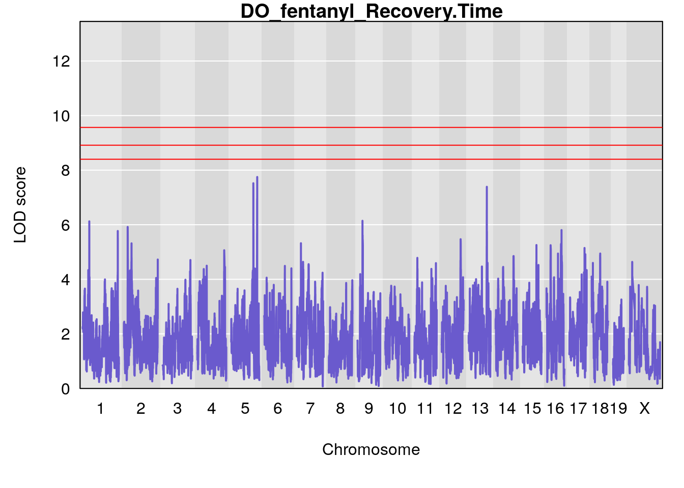
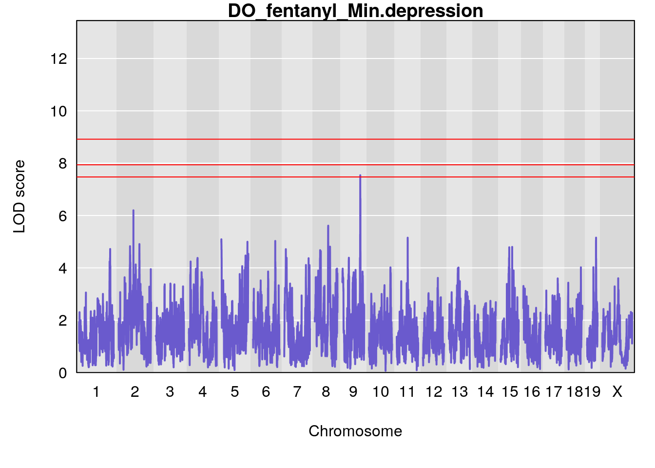
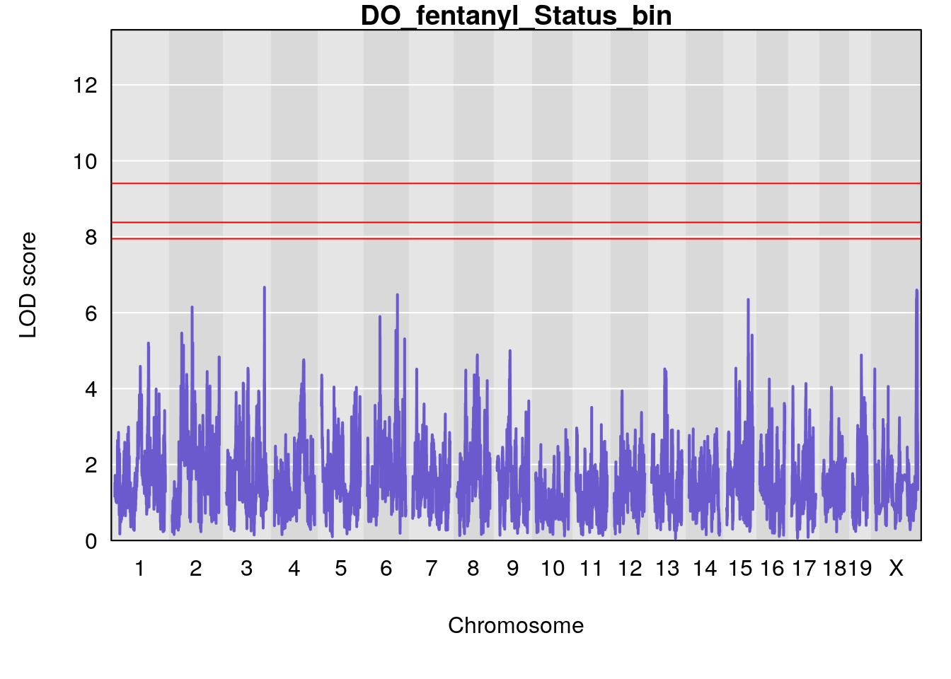
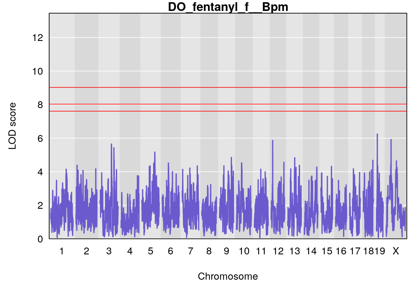
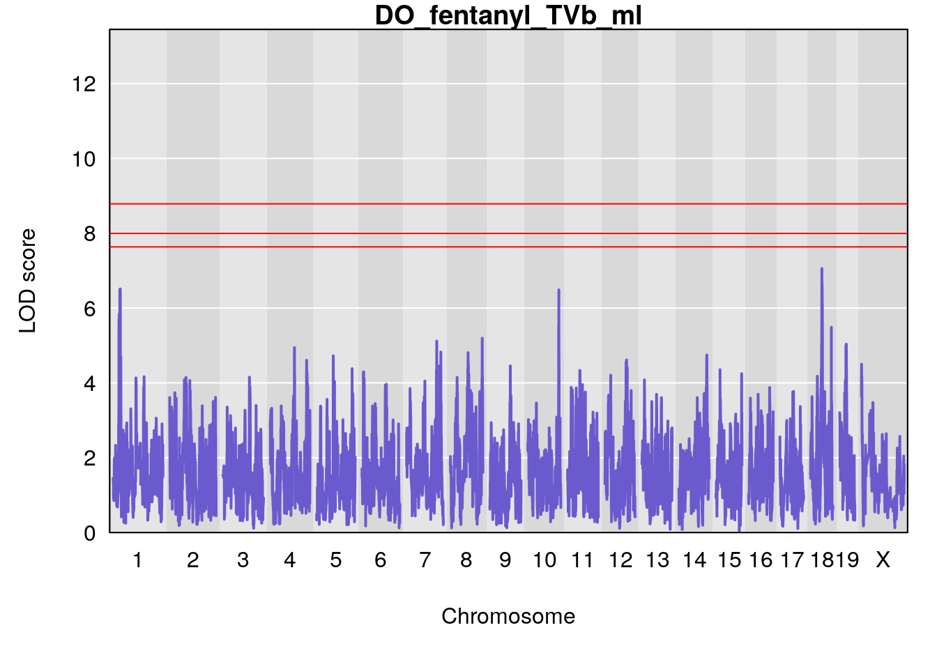
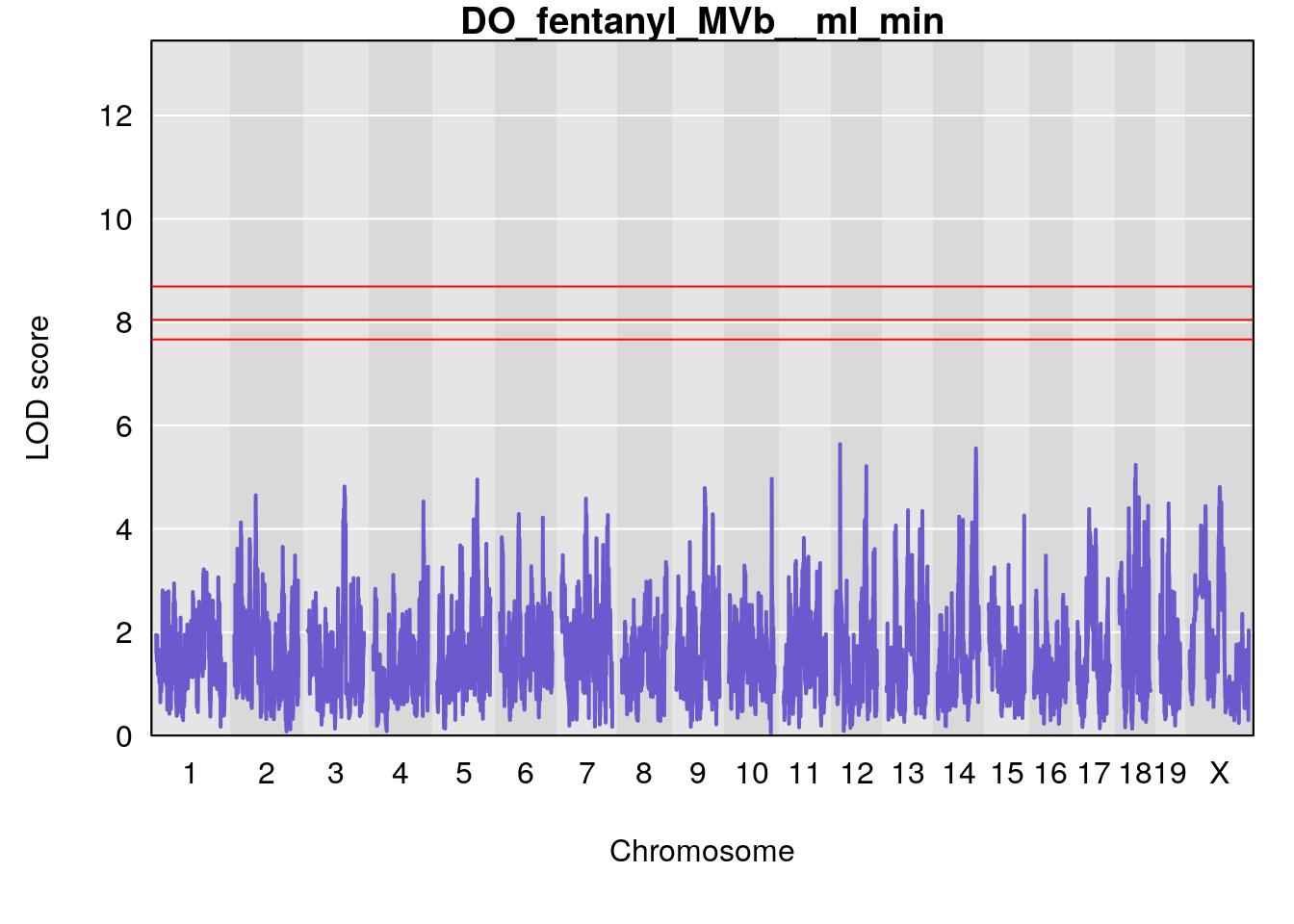
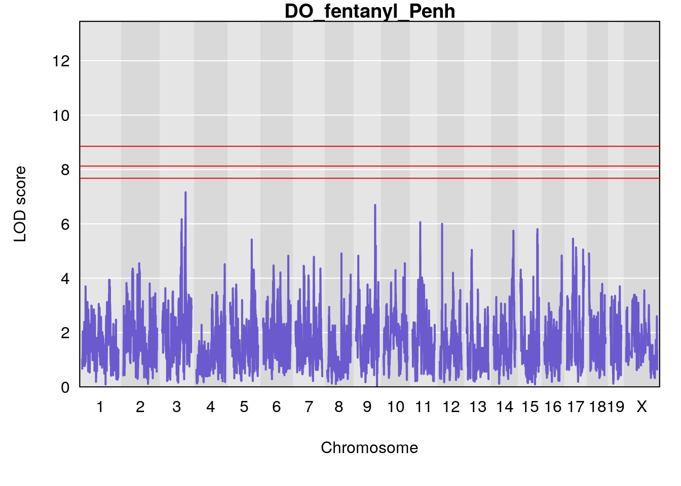
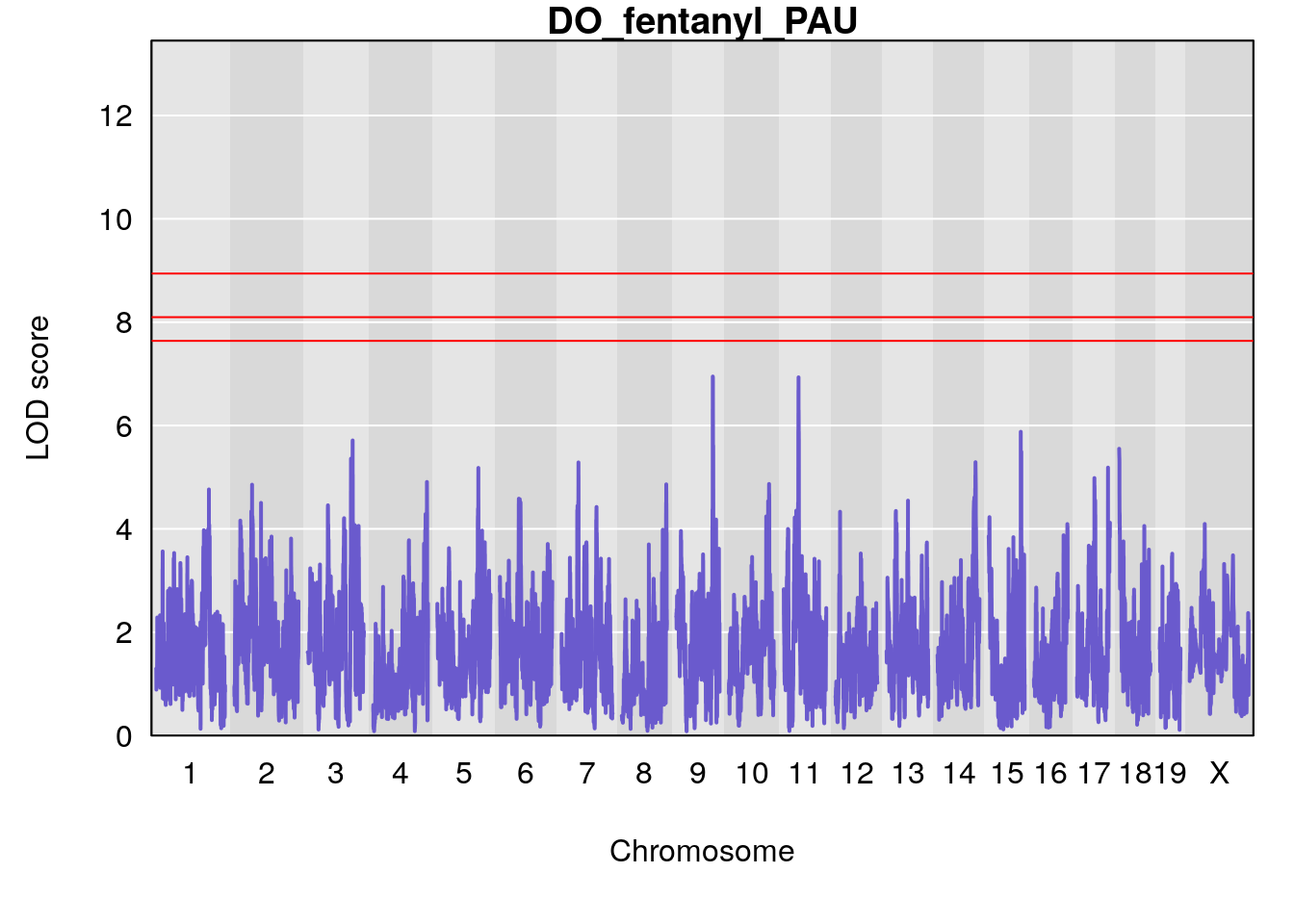
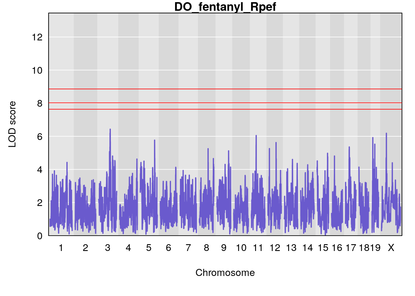
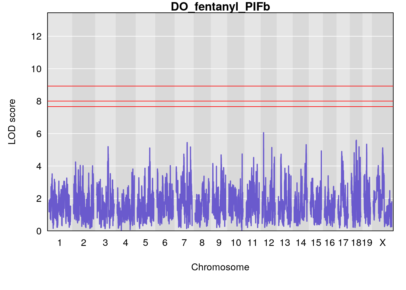

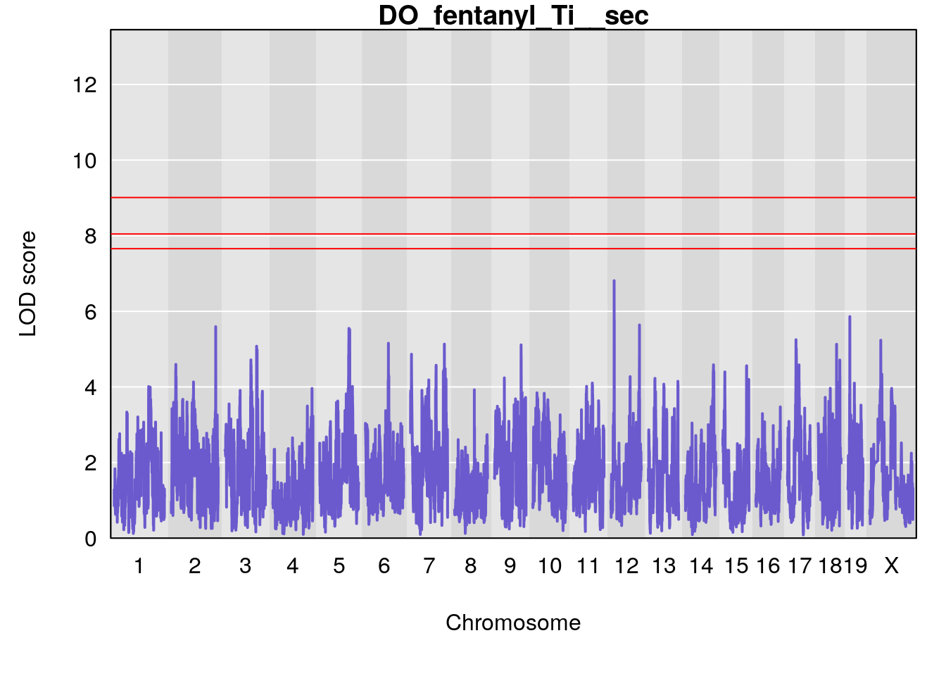
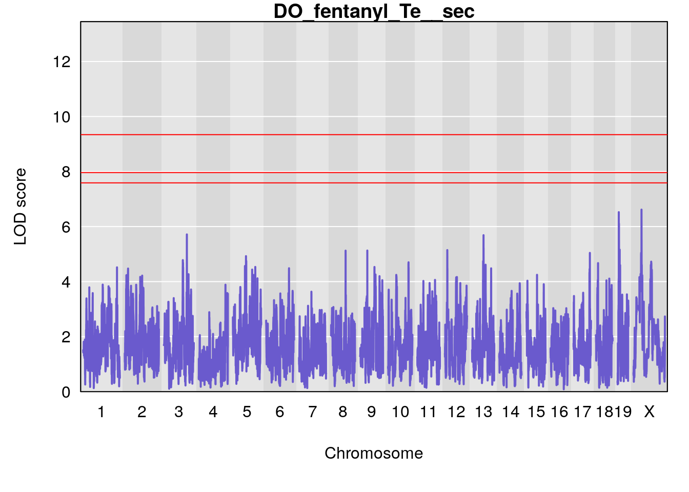

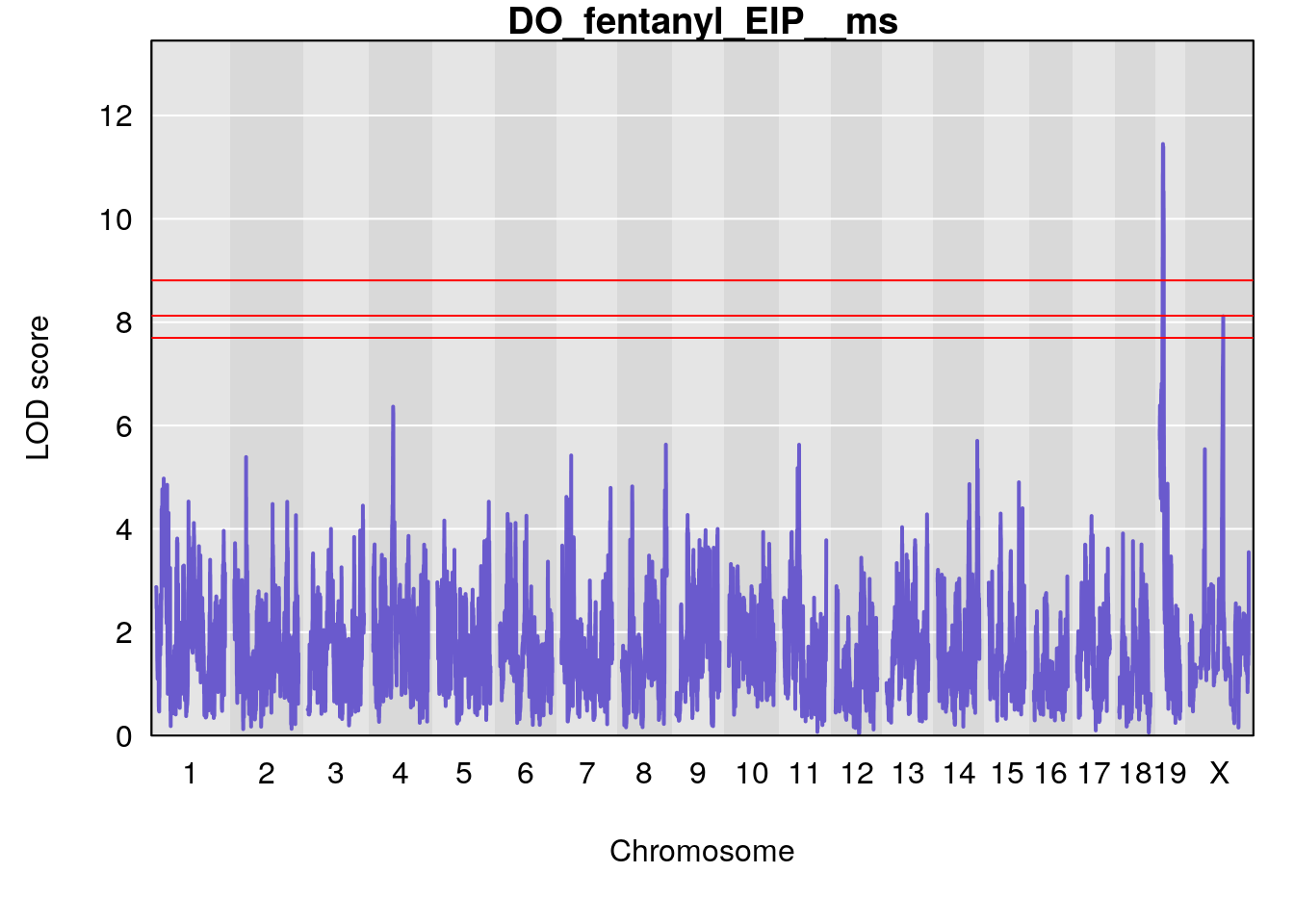
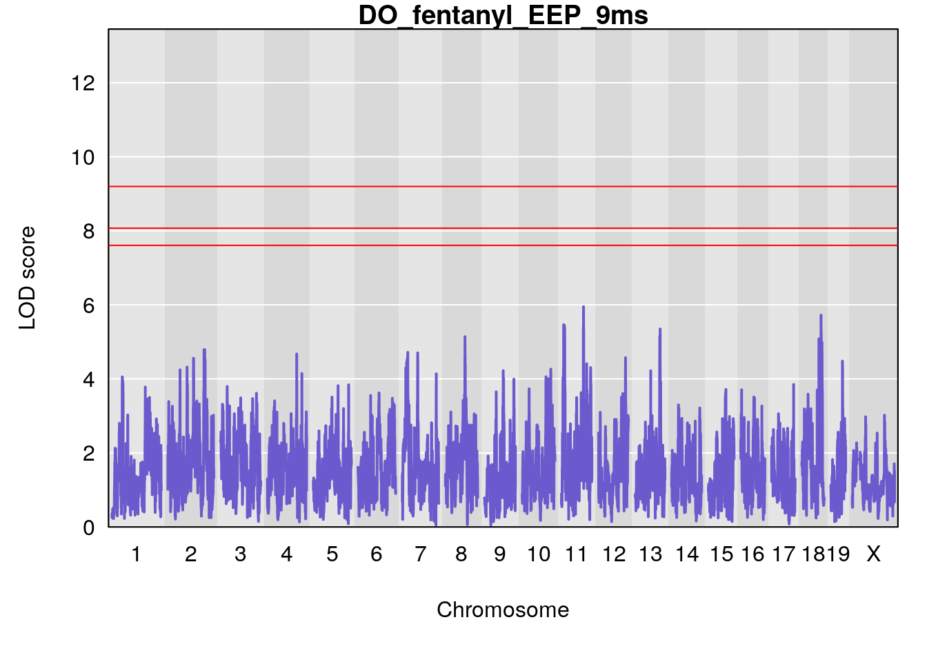
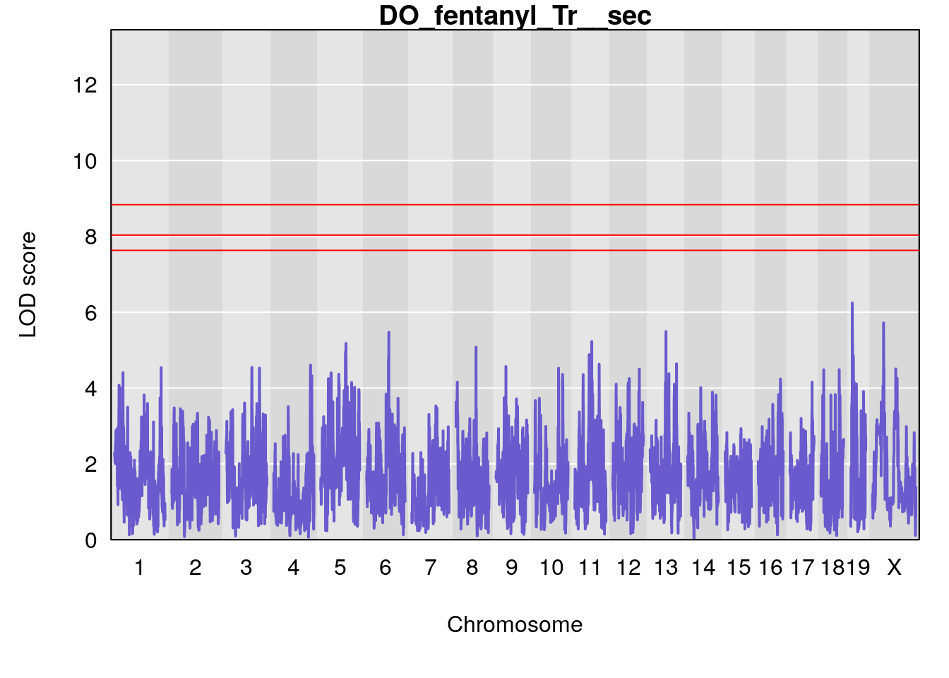
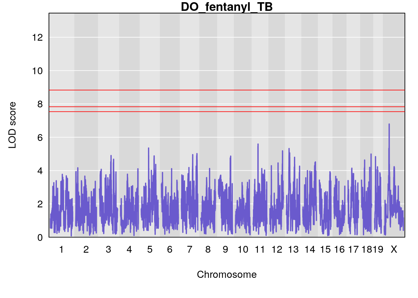
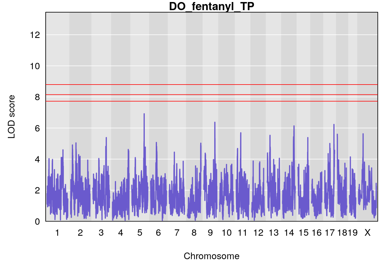
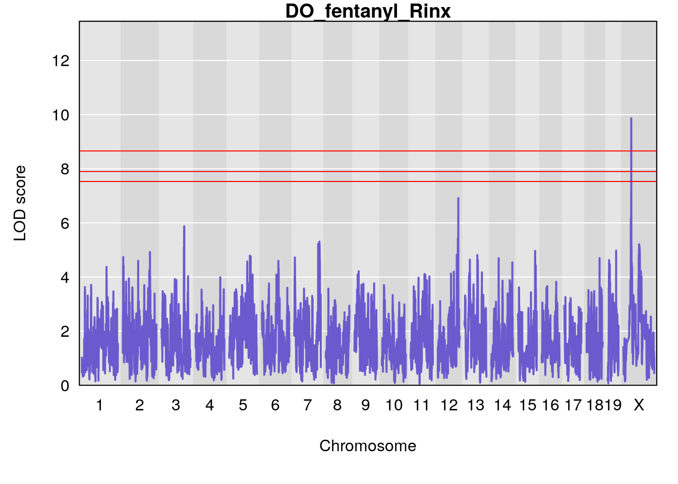
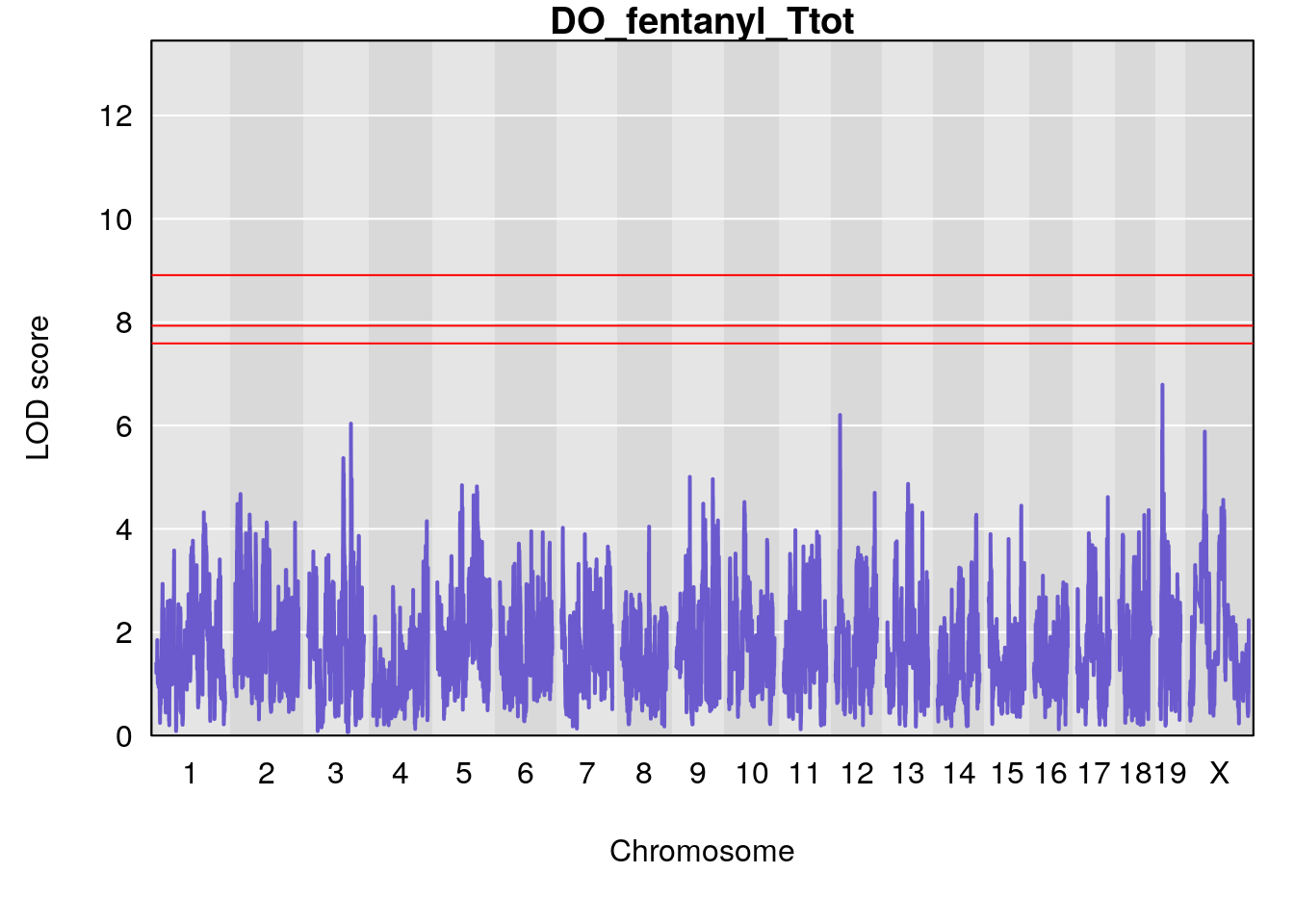
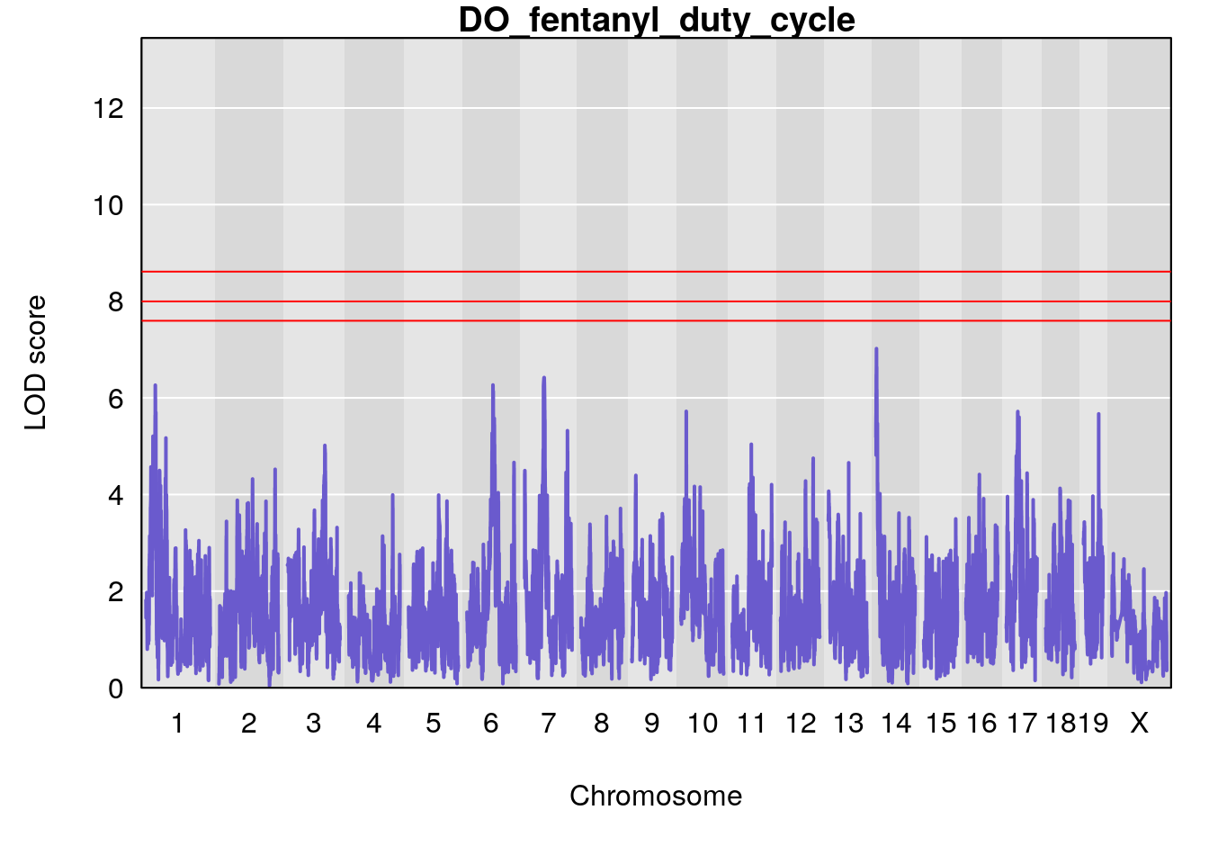
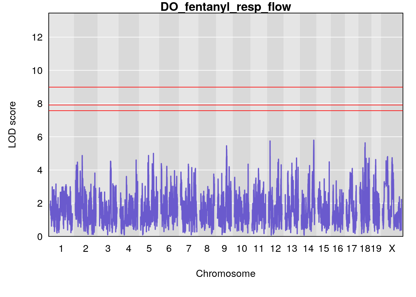


#peaks coeff plot
for(i in names(qtl.morphine.out)){
  print(i)
  peaks <- find_peaks(qtl.morphine.out[[i]], map=gm$pmap, threshold=6, drop=1.5)
  print(peaks)
  if(dim(peaks)[1] != 0){
    for(p in 1:dim(peaks)[1]) {
      print(p)
      chr <-peaks[p,3]
      #coeff plot
      par(mar=c(4.1, 4.1, 0.6, 0.6))
      plot_coefCC(coef_c1[[i]][[p]], gm$pmap[chr], scan1_output=qtl.morphine.out[[i]], bgcolor="gray95", legend=NULL)
      plot_coefCC(coef_c2[[i]][[p]], gm$pmap[chr], scan1_output=qtl.morphine.out[[i]], bgcolor="gray95", legend=NULL)
      plot(out_snps[[i]][[p]]$lod, out_snps[[i]][[p]]$snpinfo, drop_hilit=1.5, genes=out_genes[[i]][[p]])
    }
  }
}
# [1] "Survival.Time"
#   lodindex lodcolumn chr       pos      lod     ci_lo     ci_hi
# 1        1    pheno1   5 139.64055 6.173195 139.19543 140.50099
# 2        1    pheno1  12  16.64600 7.526574  16.59499  17.41229
# 3        1    pheno1  15  88.24633 7.206902  87.98976  88.27540
# 4        1    pheno1  18  68.22585 6.348355  68.19980  68.95360
# [1] 1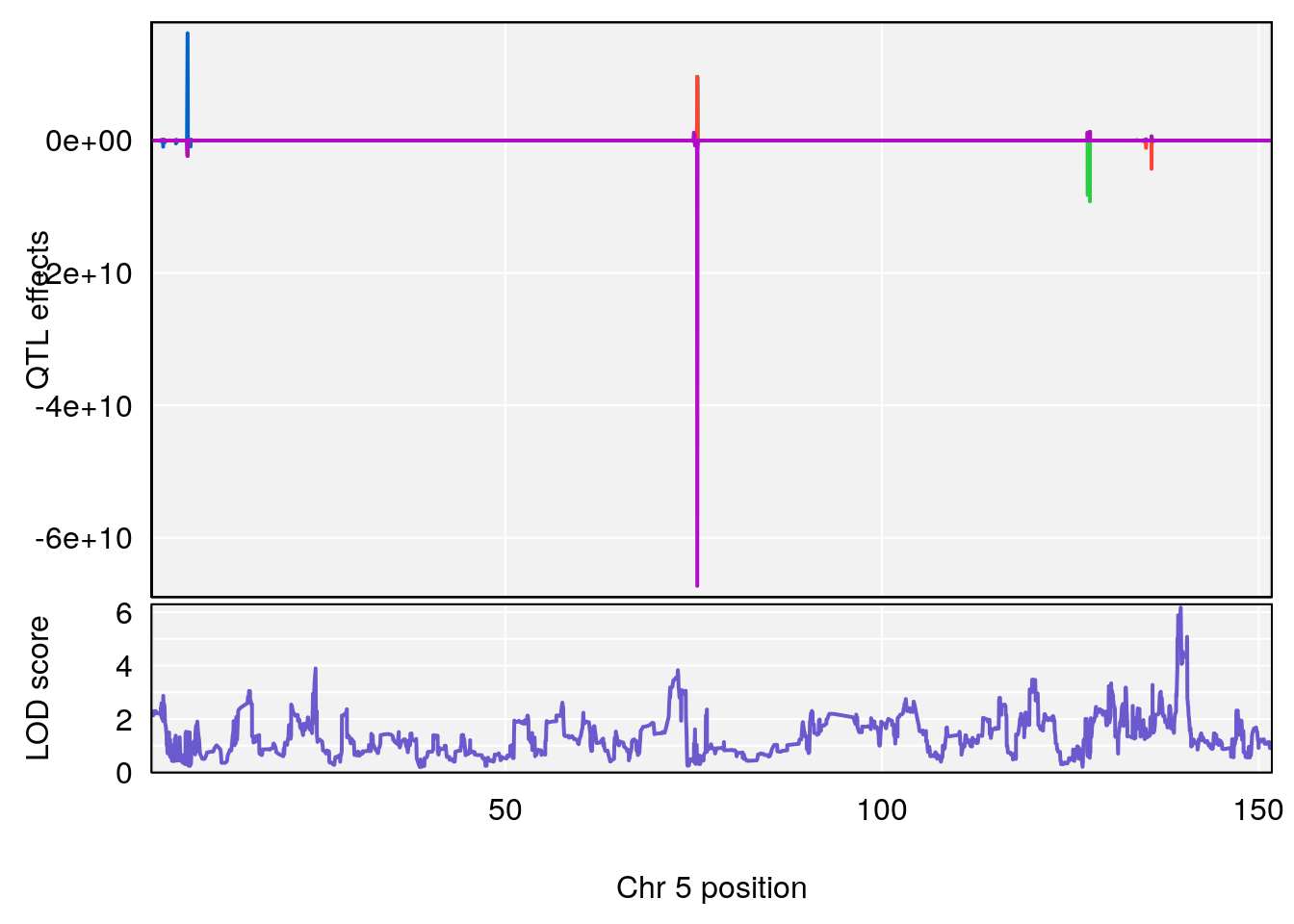
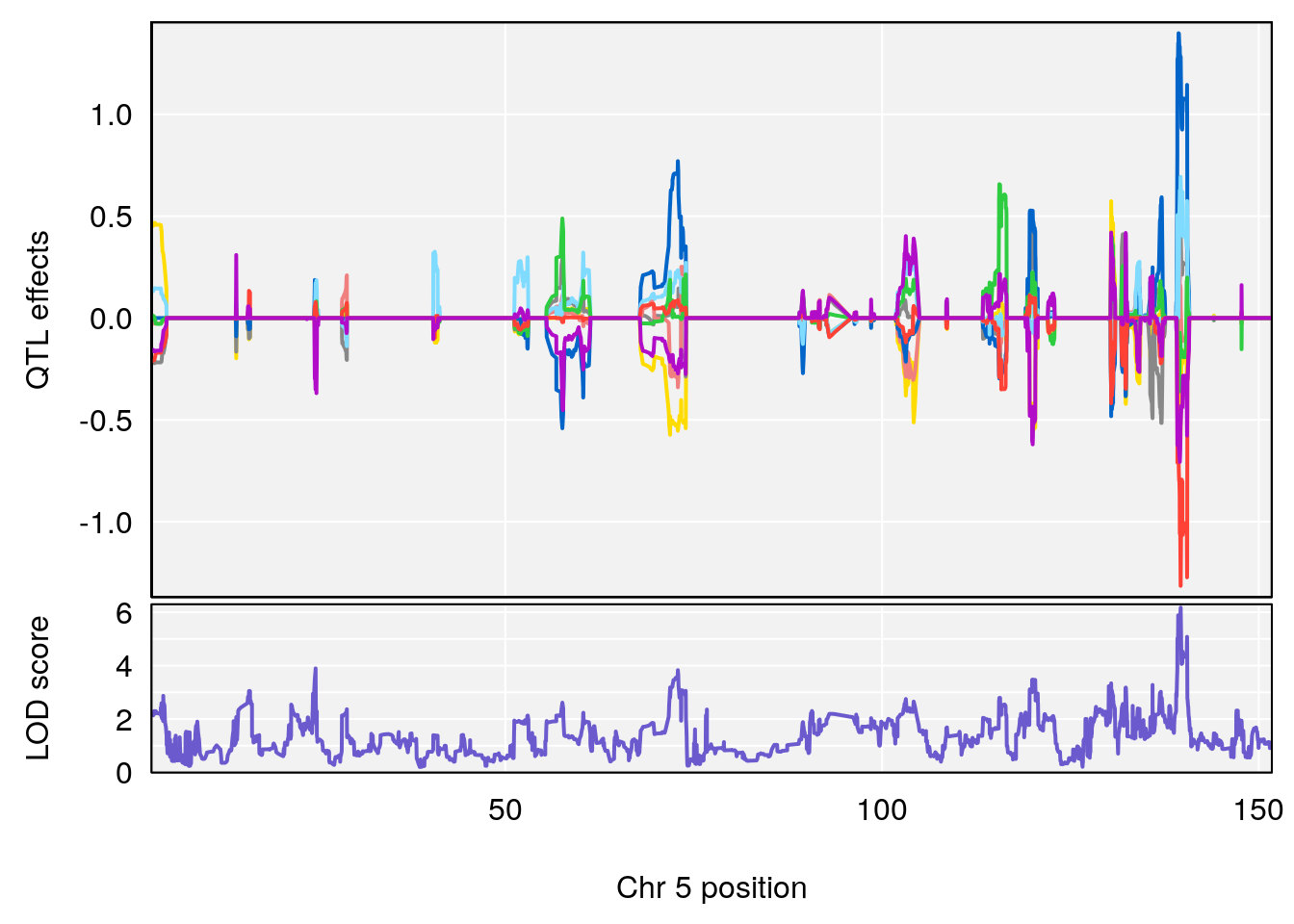
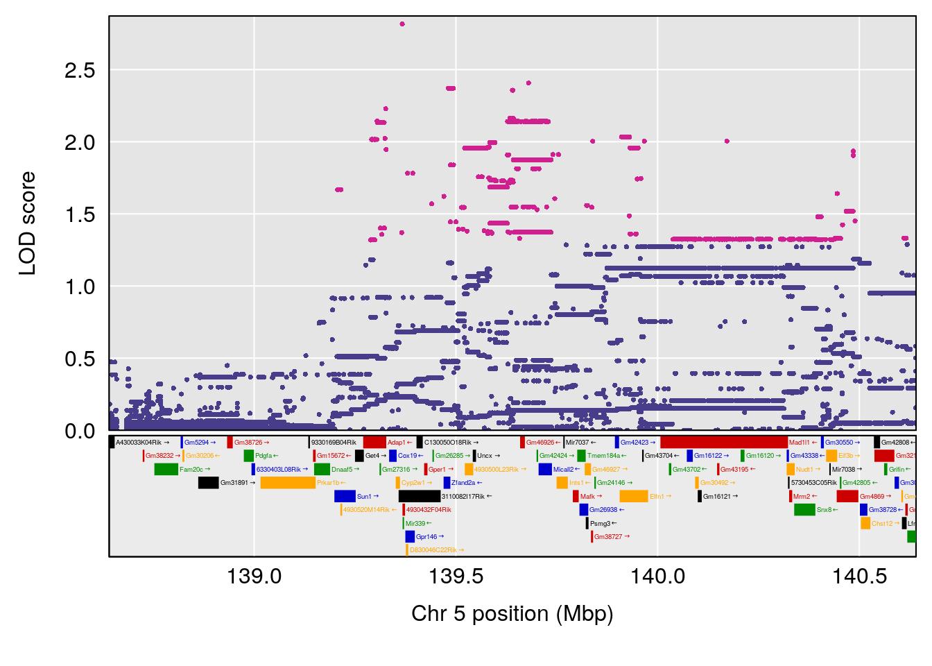
# [1] 2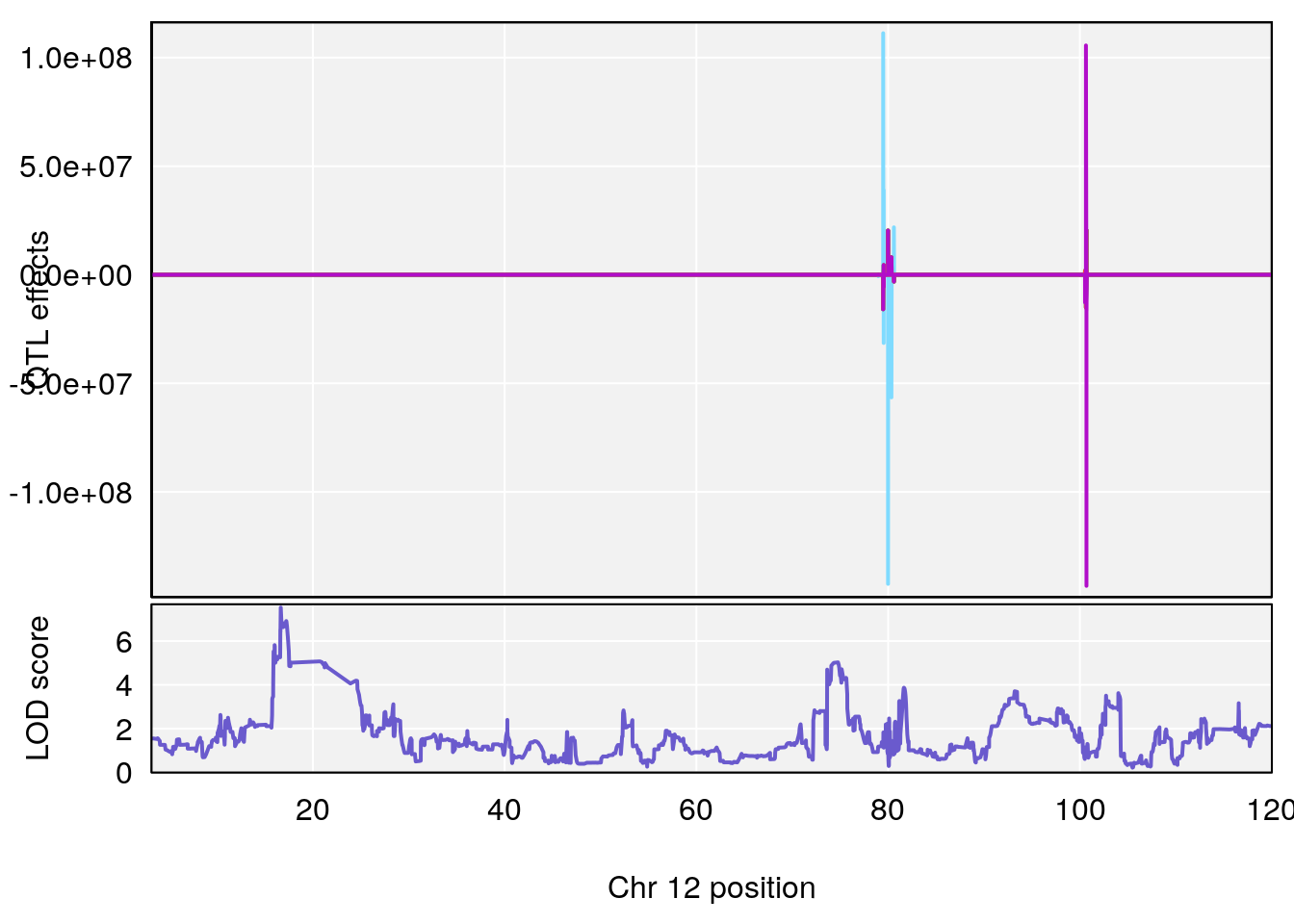
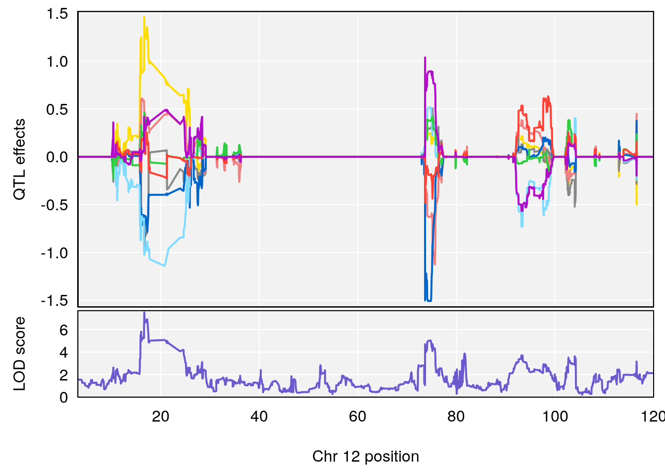
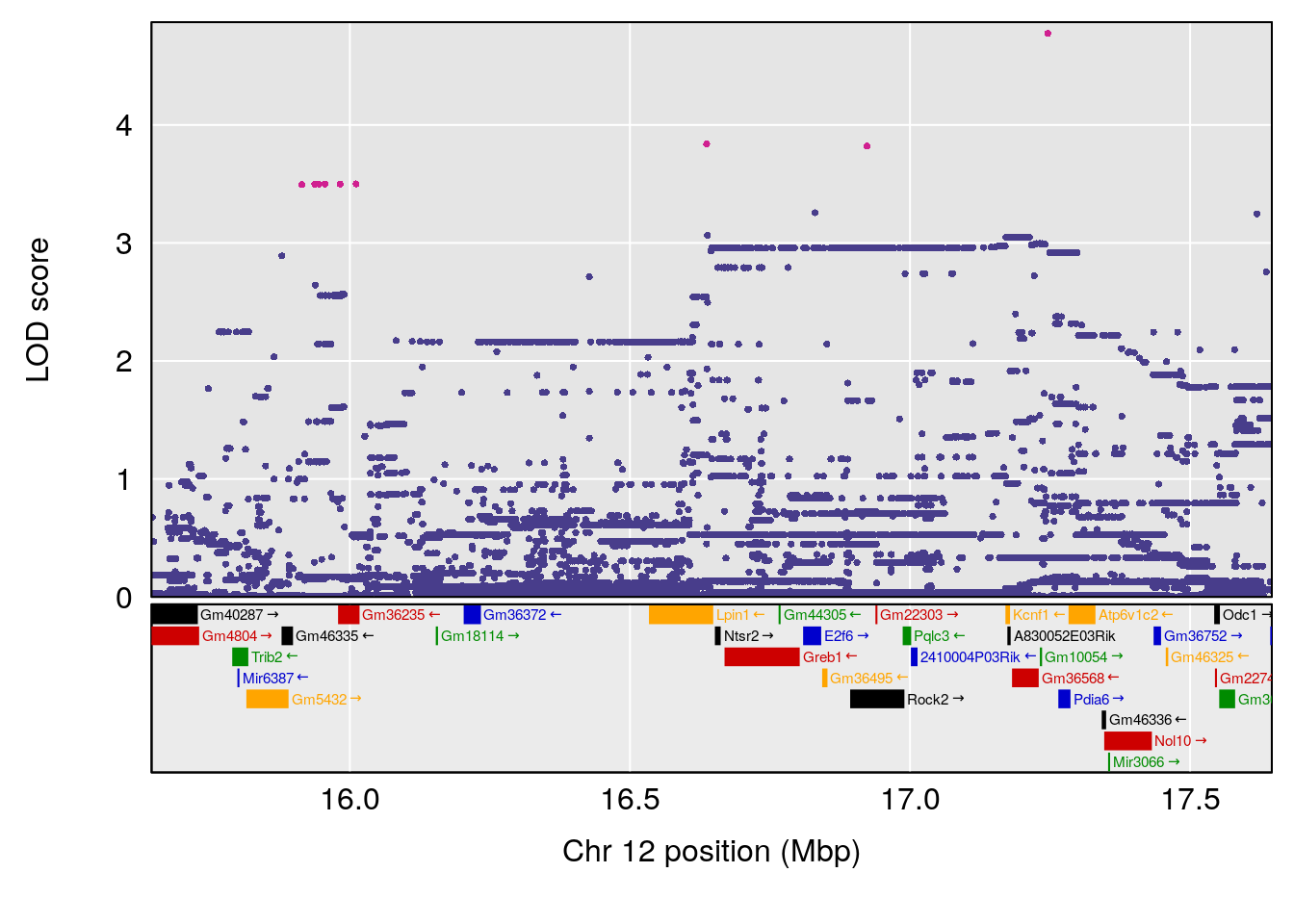
# [1] 3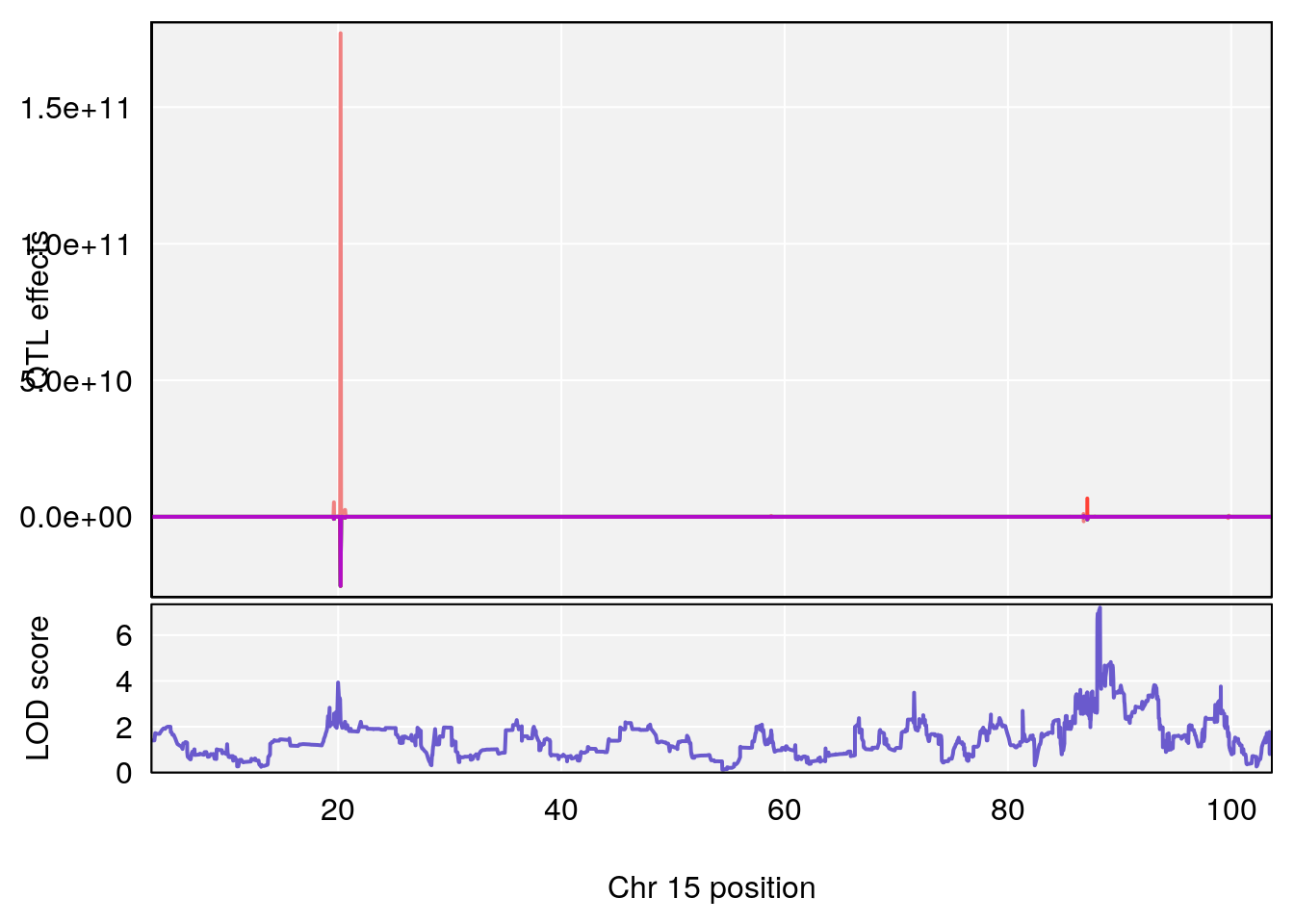
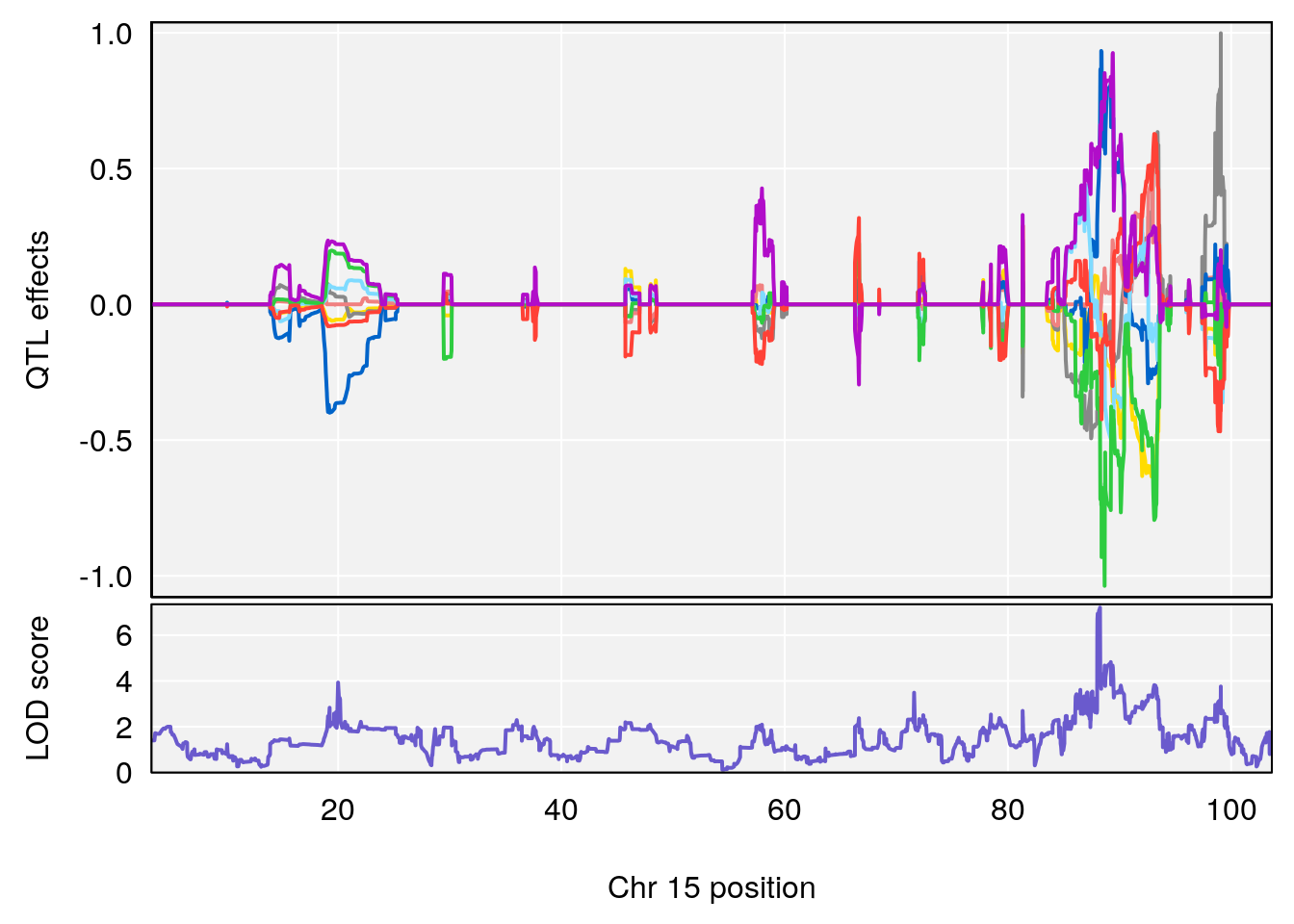
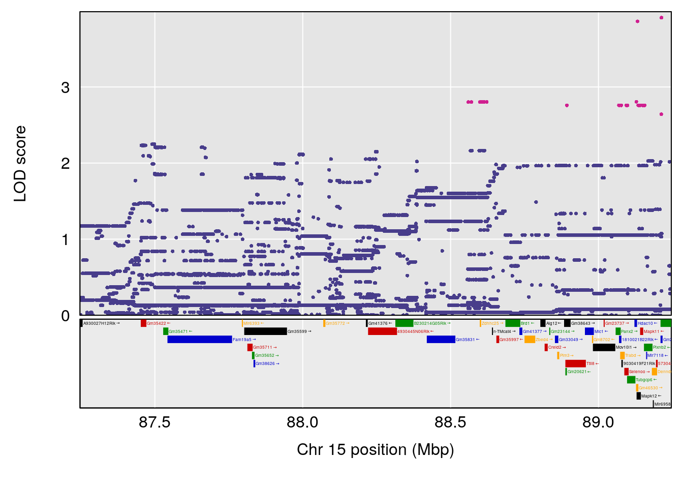
# [1] 4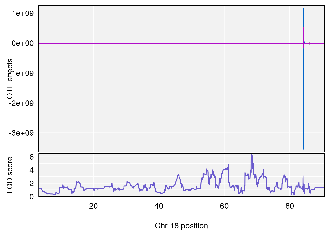
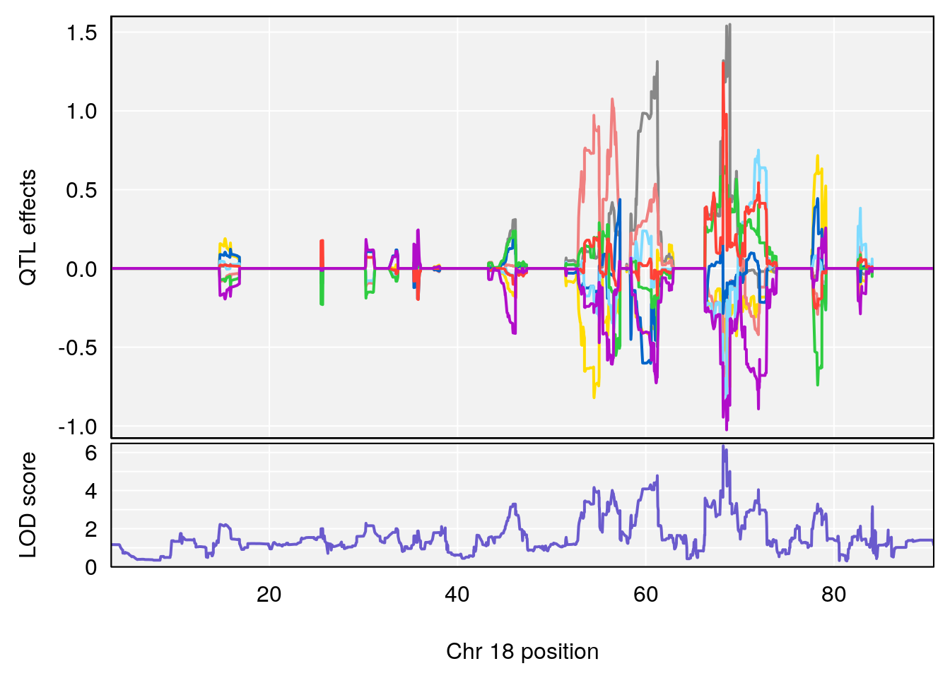
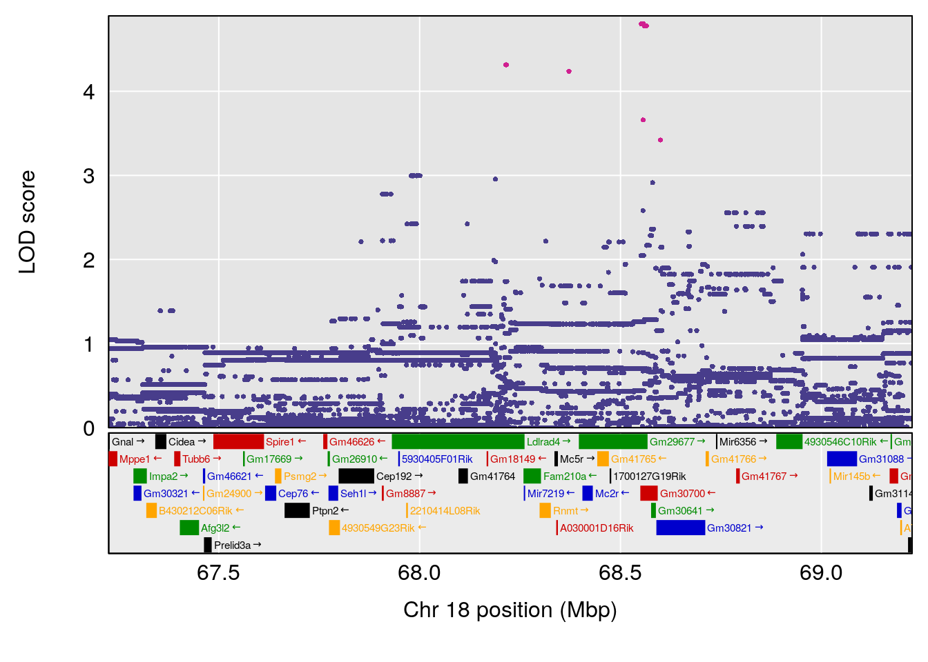
# [1] "Recovery.Time"
#   lodindex lodcolumn chr       pos      lod     ci_lo     ci_hi
# 1        1    pheno1   1  38.68137 6.123819  38.62390 189.09796
# 2        1    pheno1   5 140.48497 7.748969 119.95049 140.52523
# 3        1    pheno1   9  29.75246 6.143645  29.51025  31.87659
# 4        1    pheno1  13  99.09432 7.389577  98.69631  99.12643
# [1] 1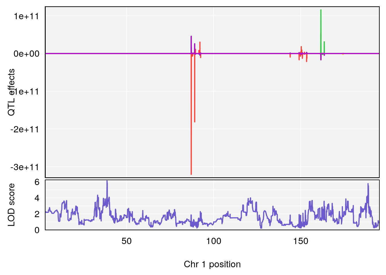
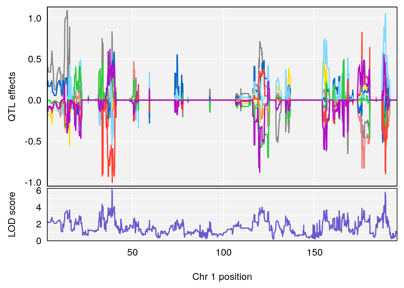
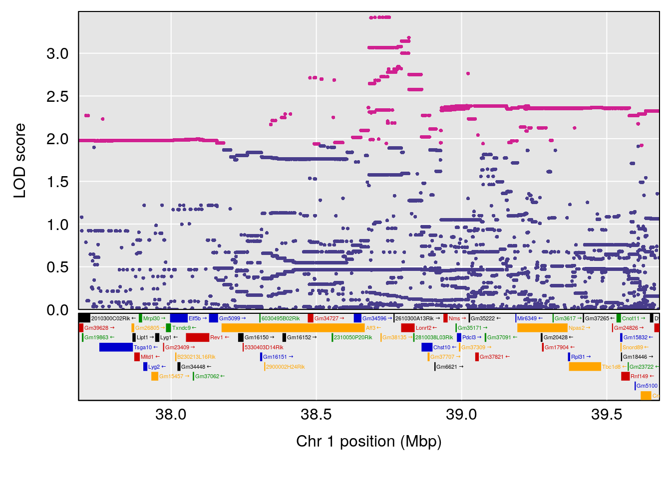
# [1] 2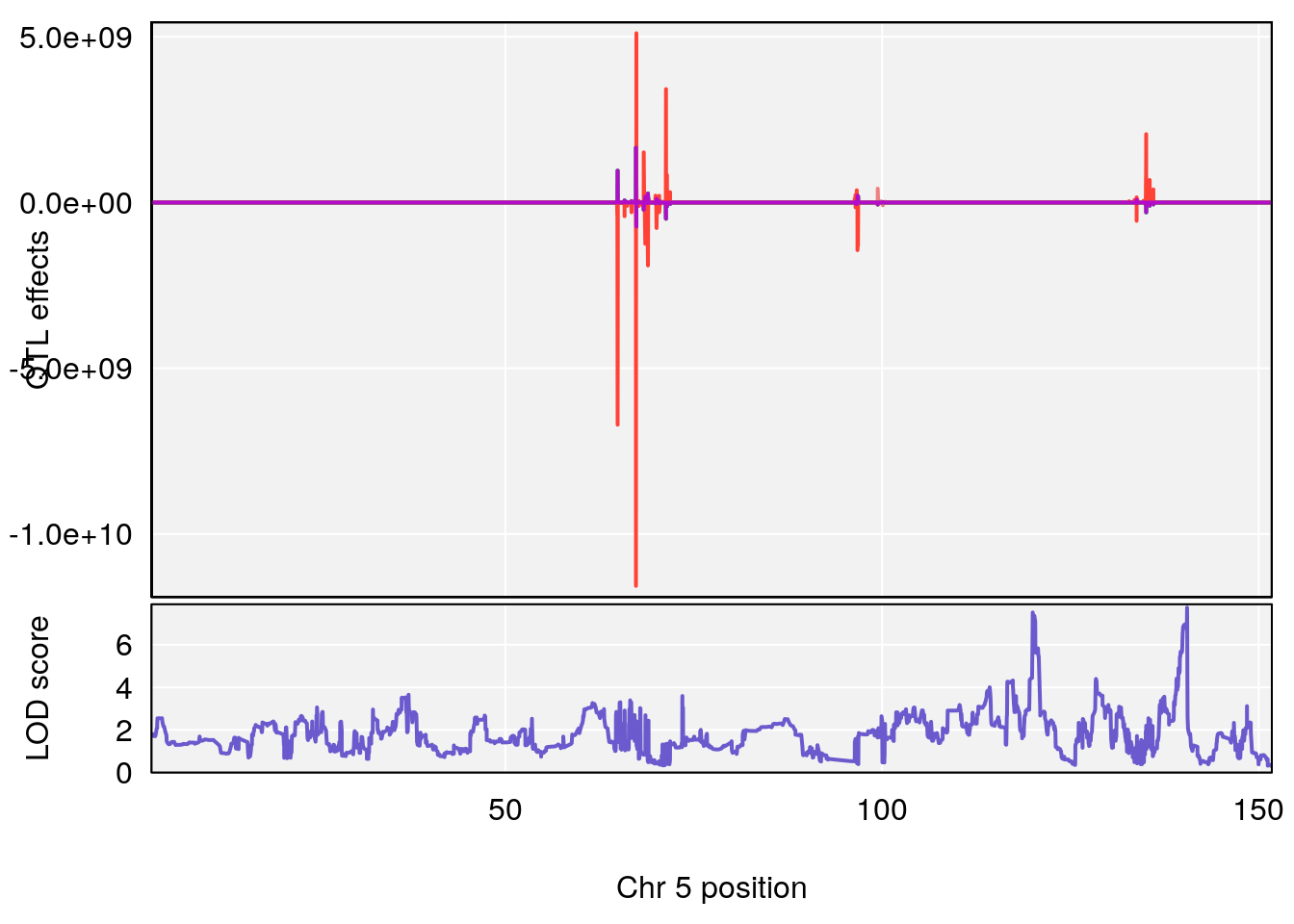
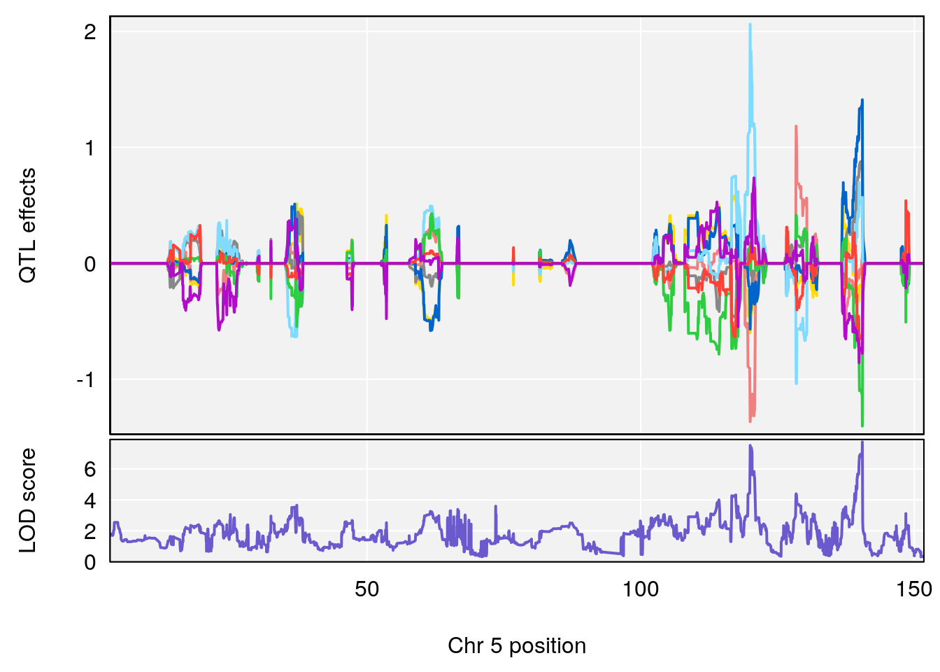
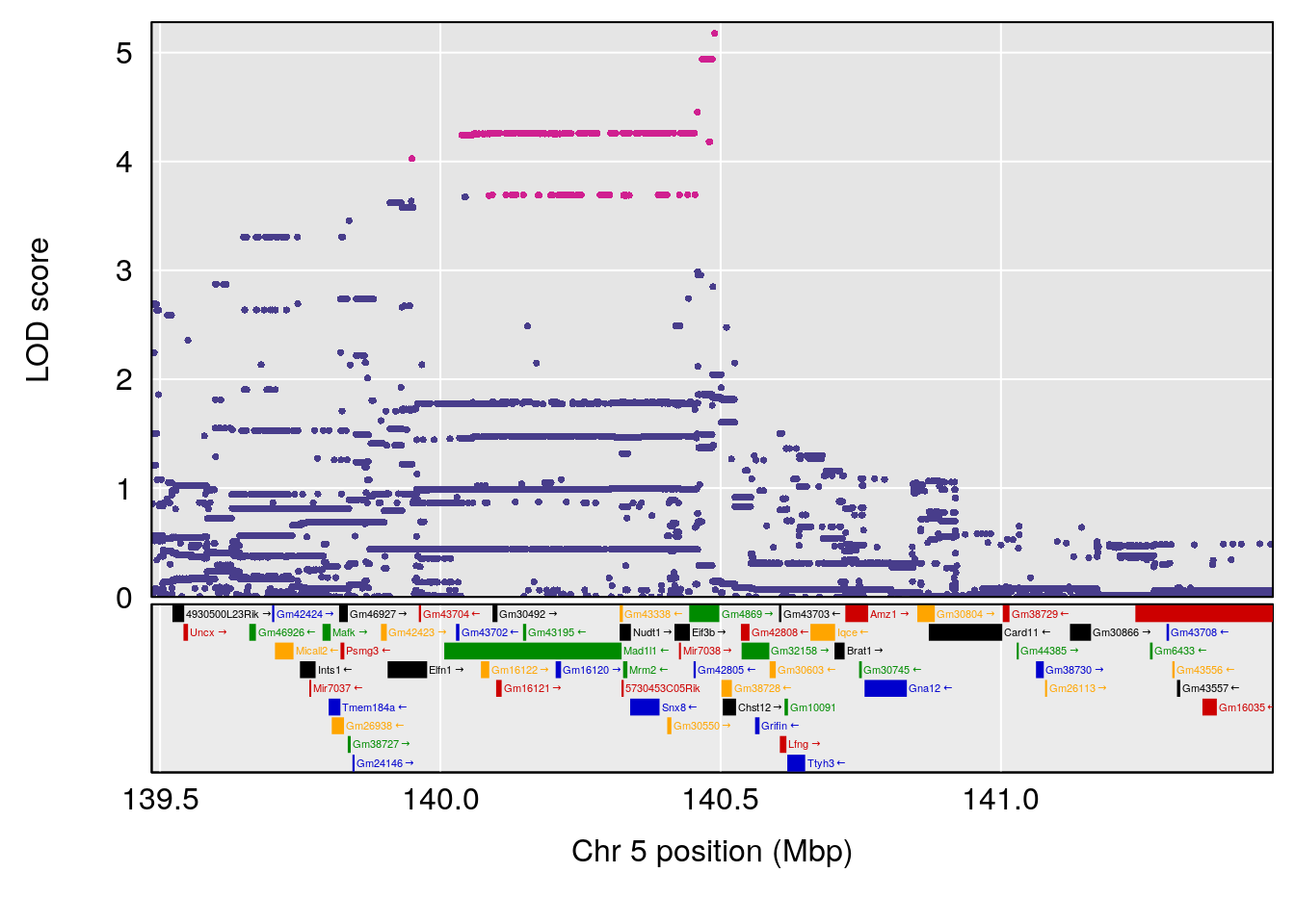
# [1] 3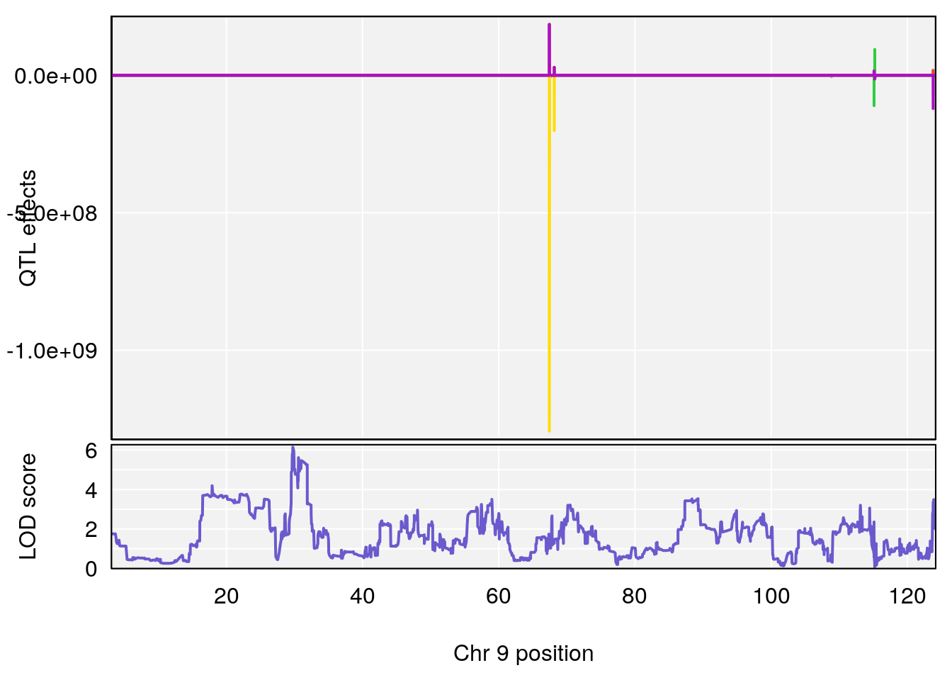
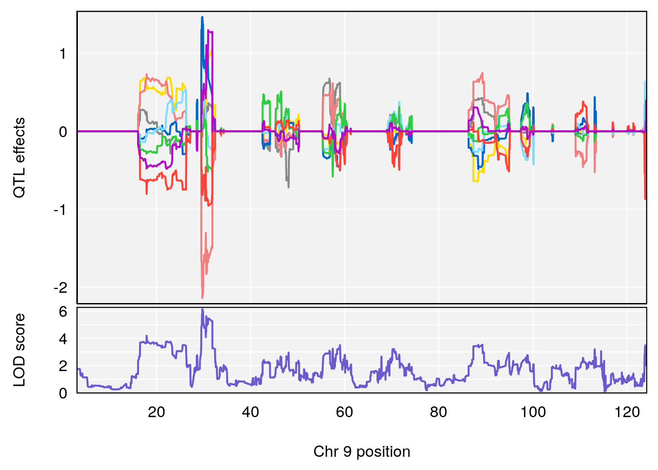
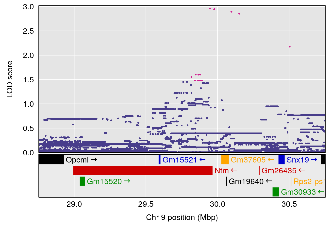
# [1] 4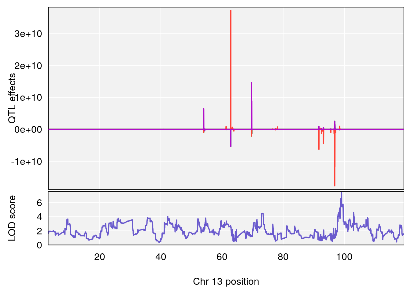
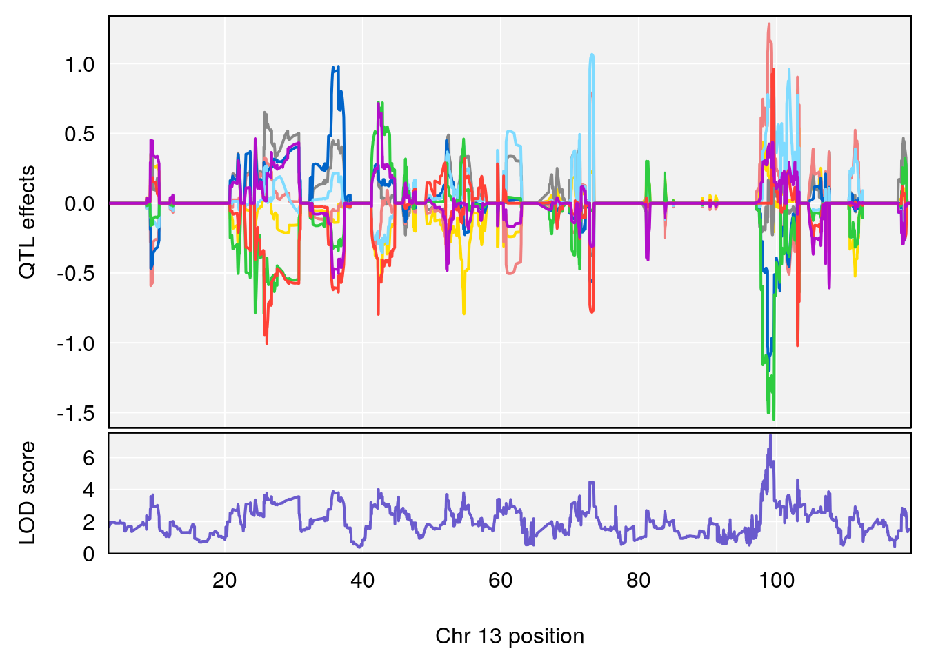
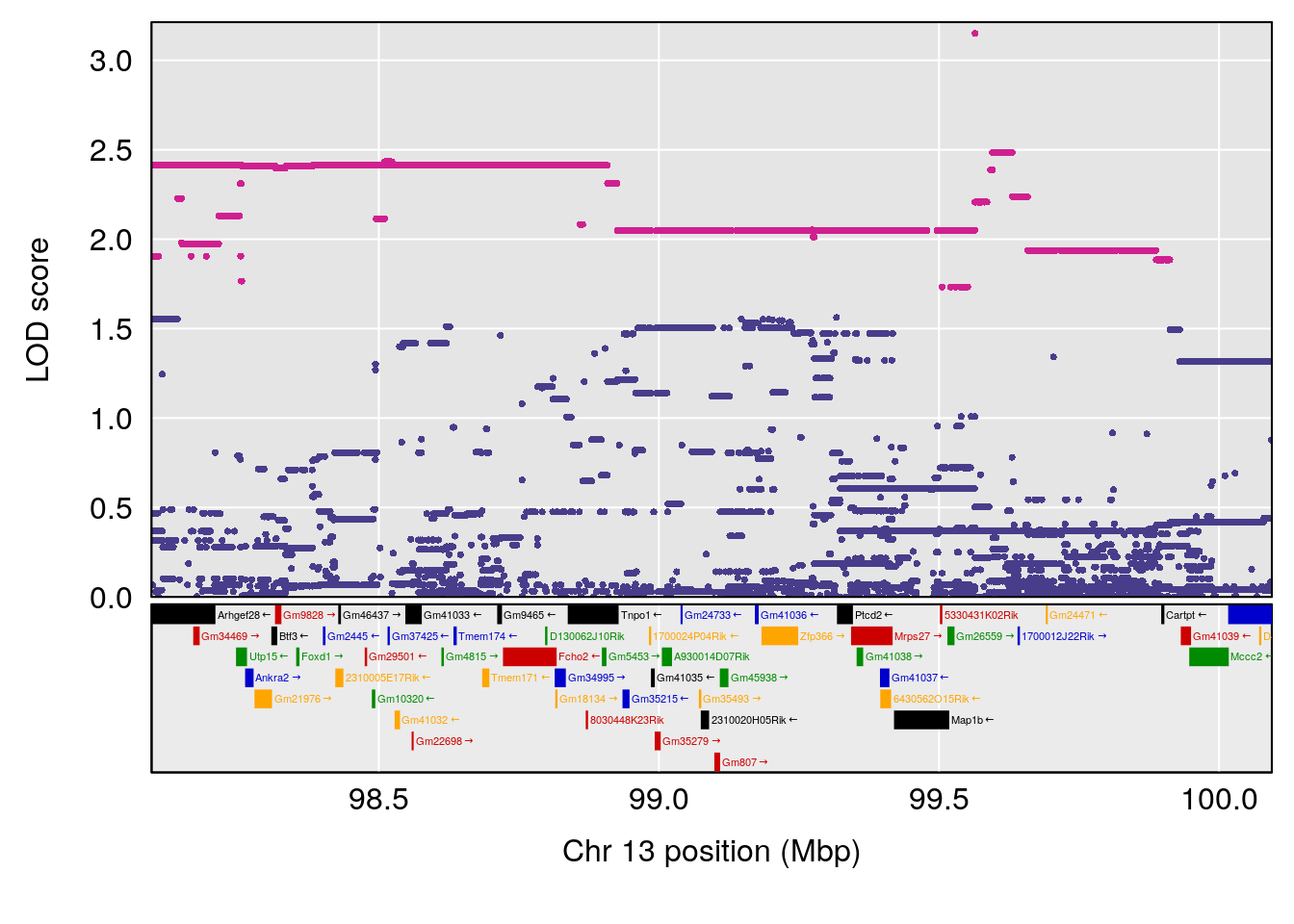
# [1] "Min.depression"
#   lodindex lodcolumn chr      pos      lod     ci_lo    ci_hi
# 1        1    pheno1   2  84.6274 6.198704  65.80752 117.8273
# 2        1    pheno1   9 102.1397 7.538969 101.91837 103.0599
# [1] 1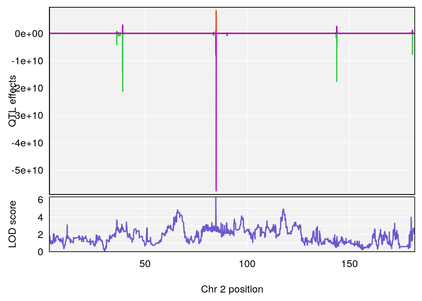
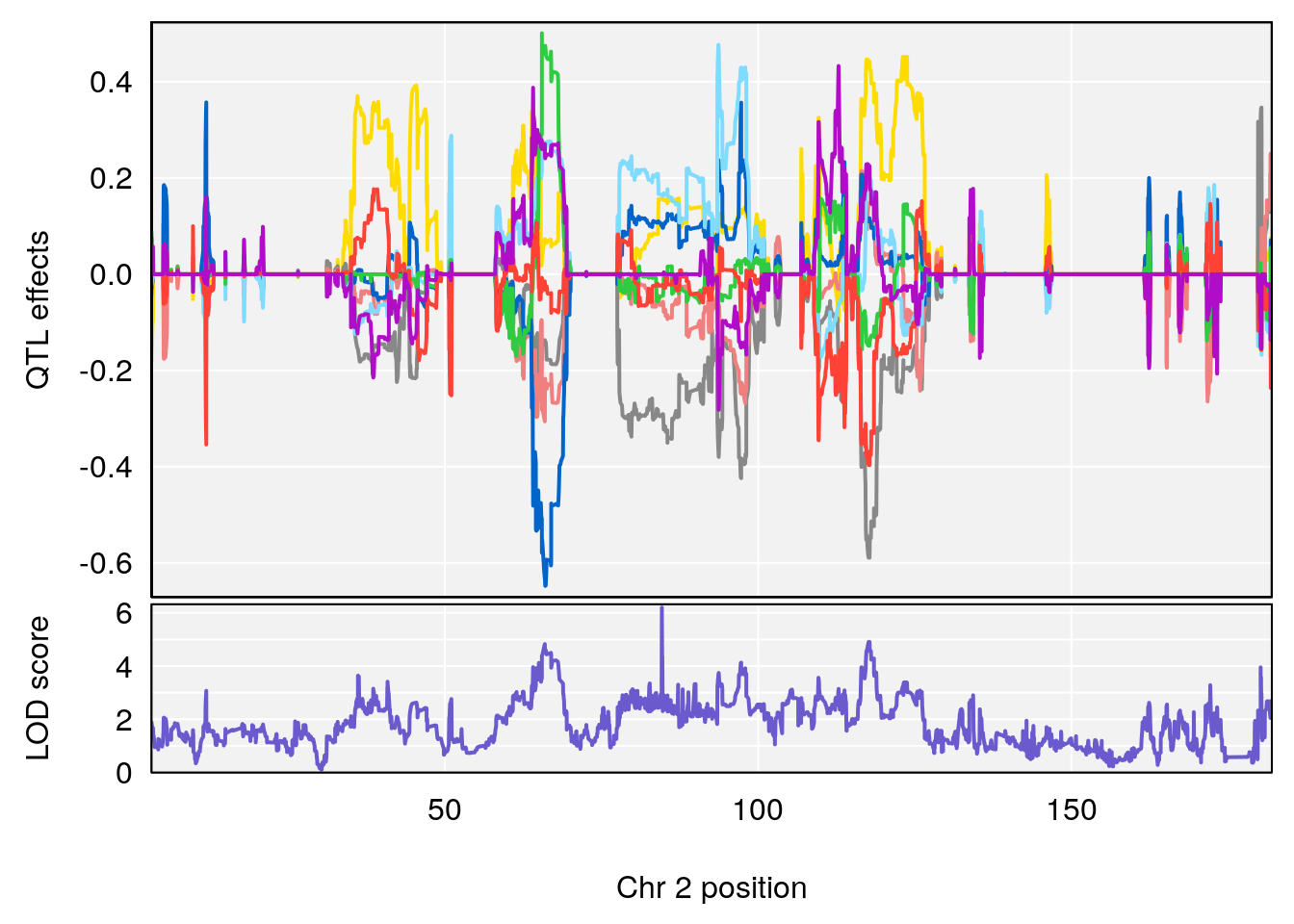
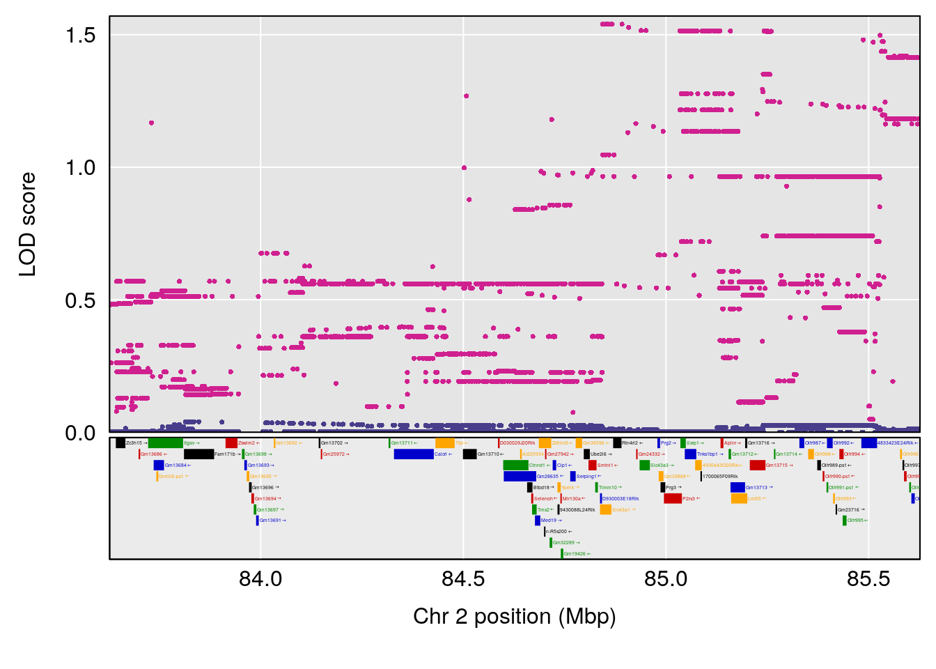
# [1] 2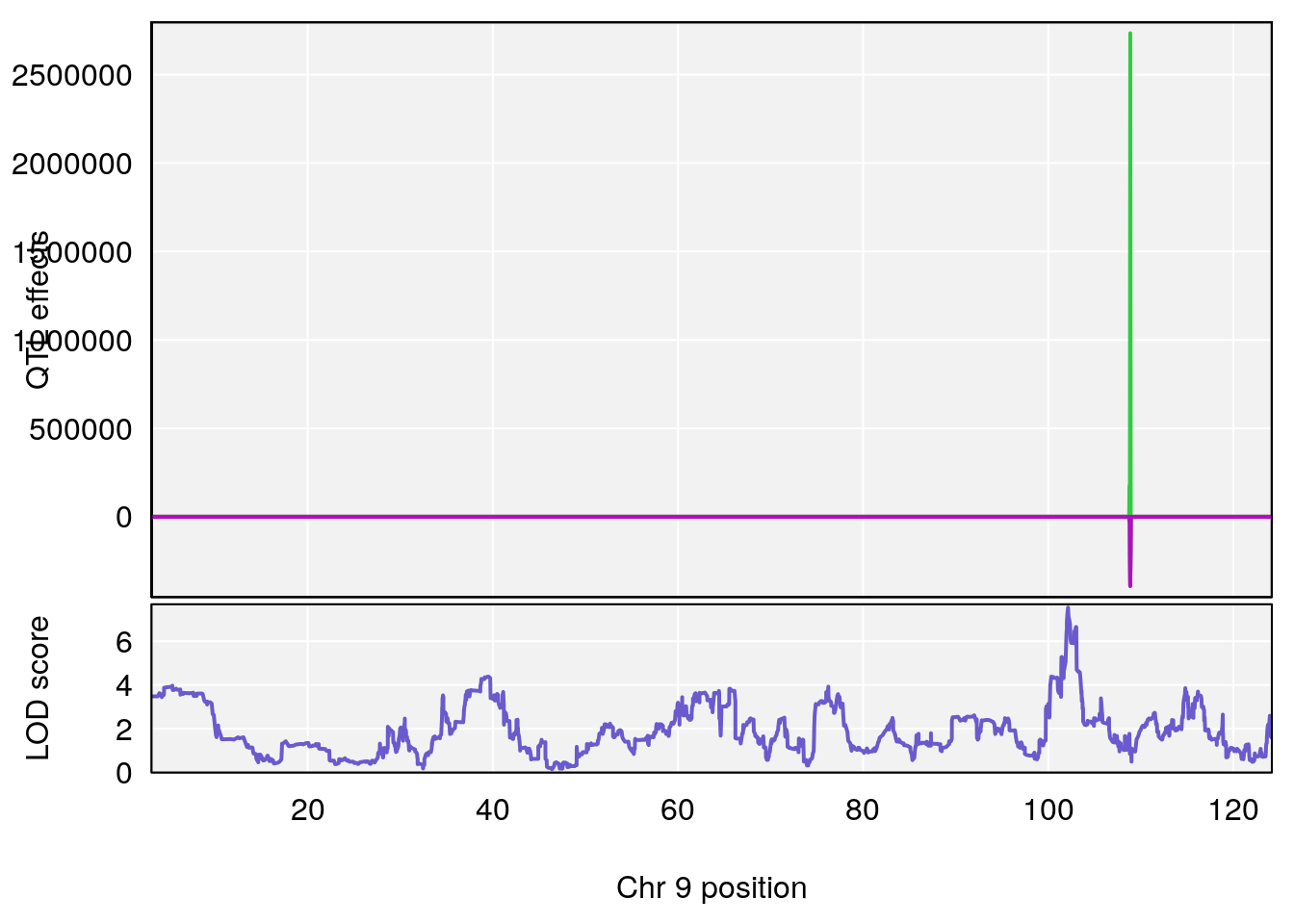
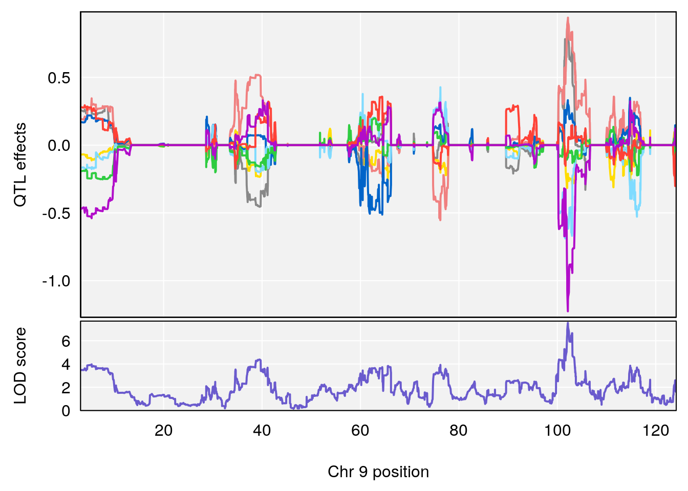
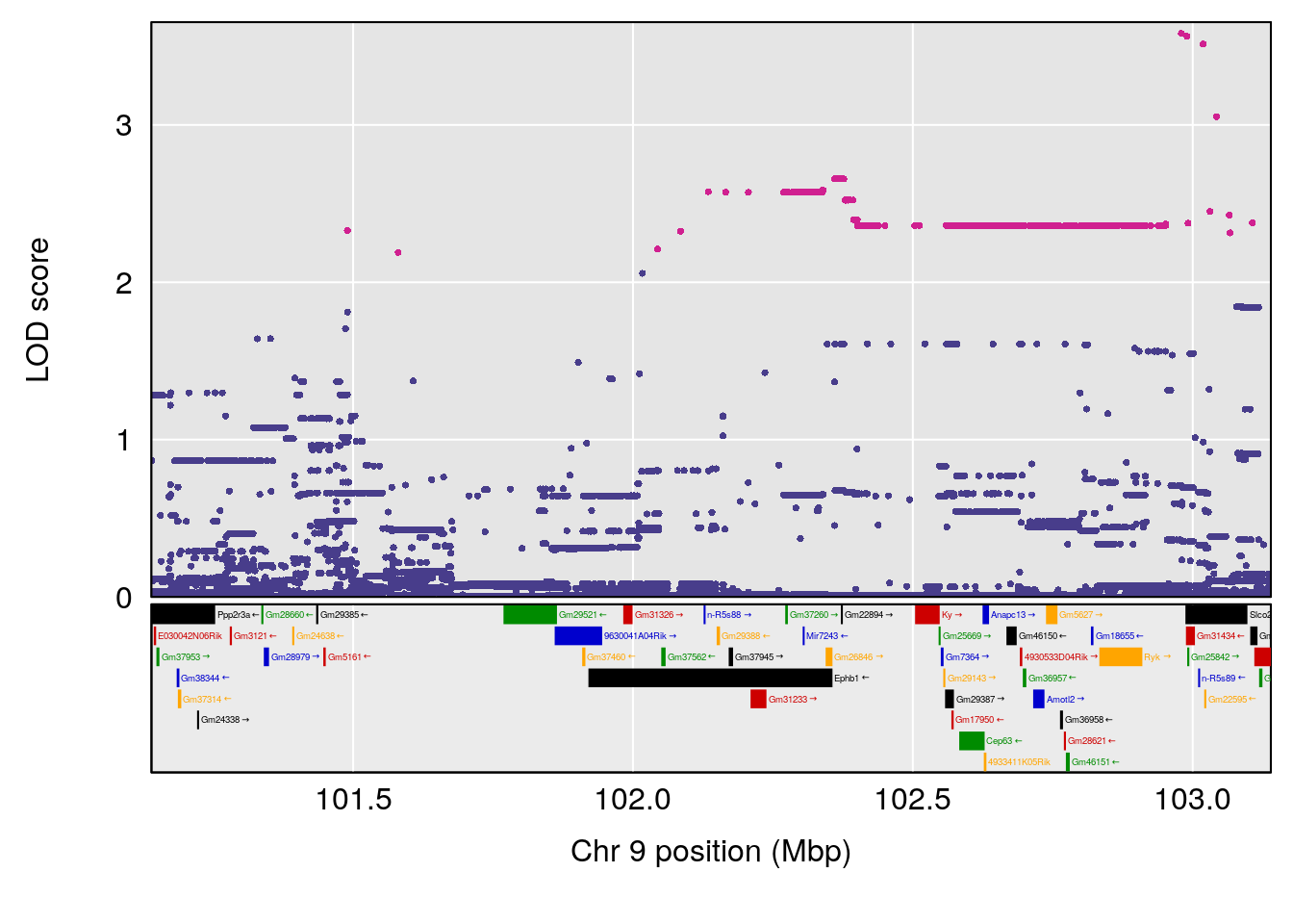
# [1] "Status_bin"
#   lodindex lodcolumn chr       pos      lod     ci_lo     ci_hi
# 1        1    pheno1   2  78.67115 6.148793  39.21518 181.80986
# 2        1    pheno1   3 148.41059 6.667905 148.23602 148.63025
# 3        1    pheno1   6 117.32940 6.475925  50.87023 144.61513
# 4        1    pheno1  15  85.38237 6.348278  85.15868  99.85481
# 5        1    pheno1   X 166.33786 6.596858 164.40631 168.30147
# [1] 1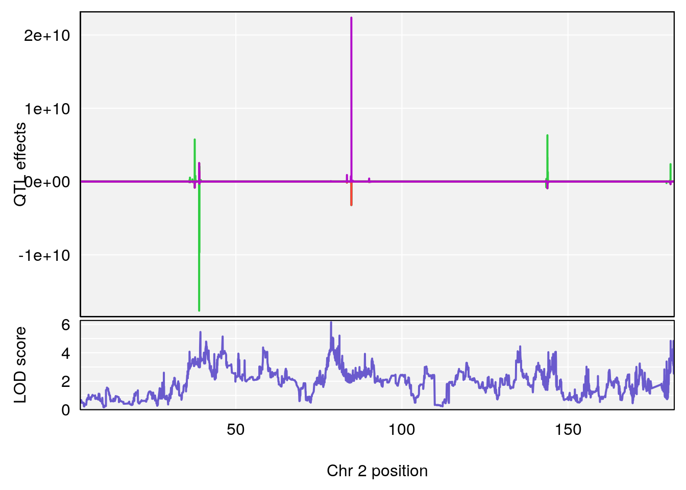
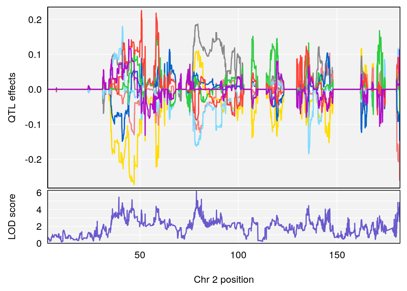
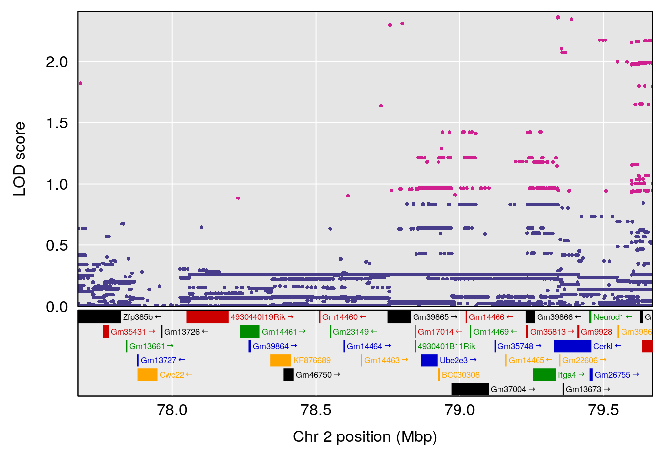
# [1] 2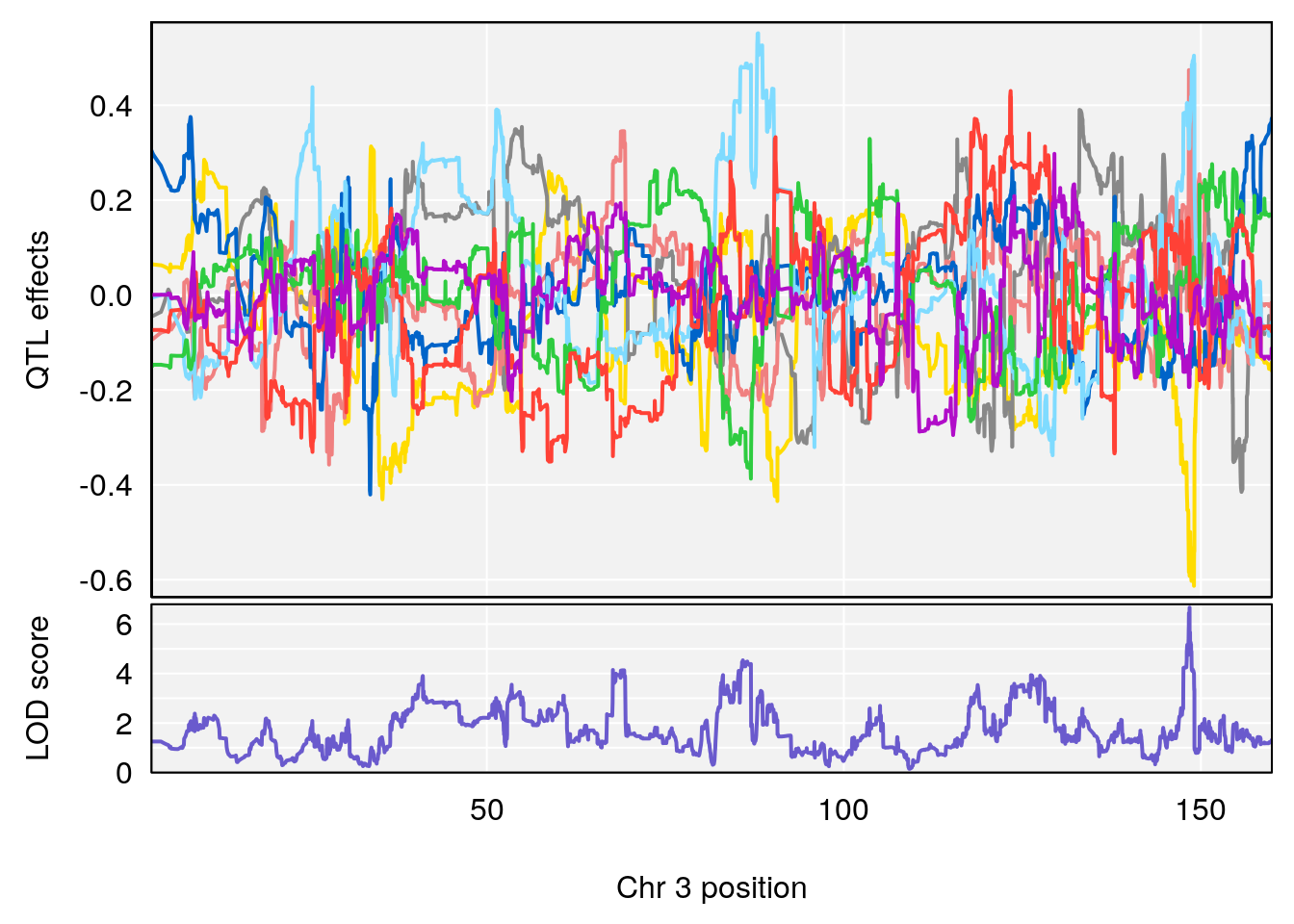
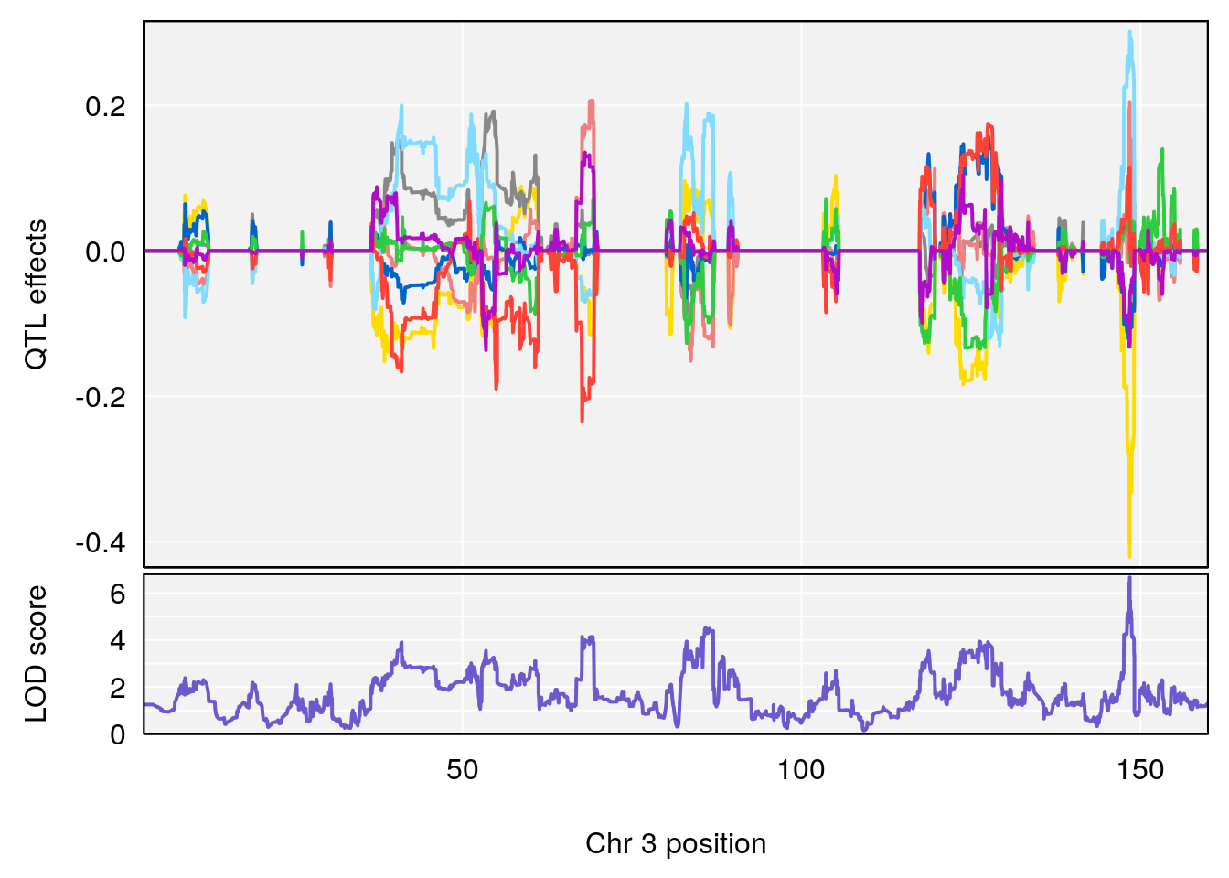
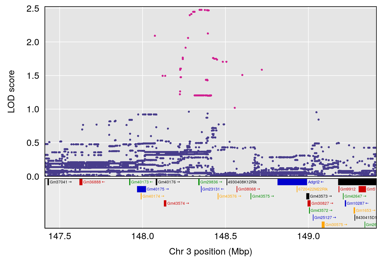
# [1] 3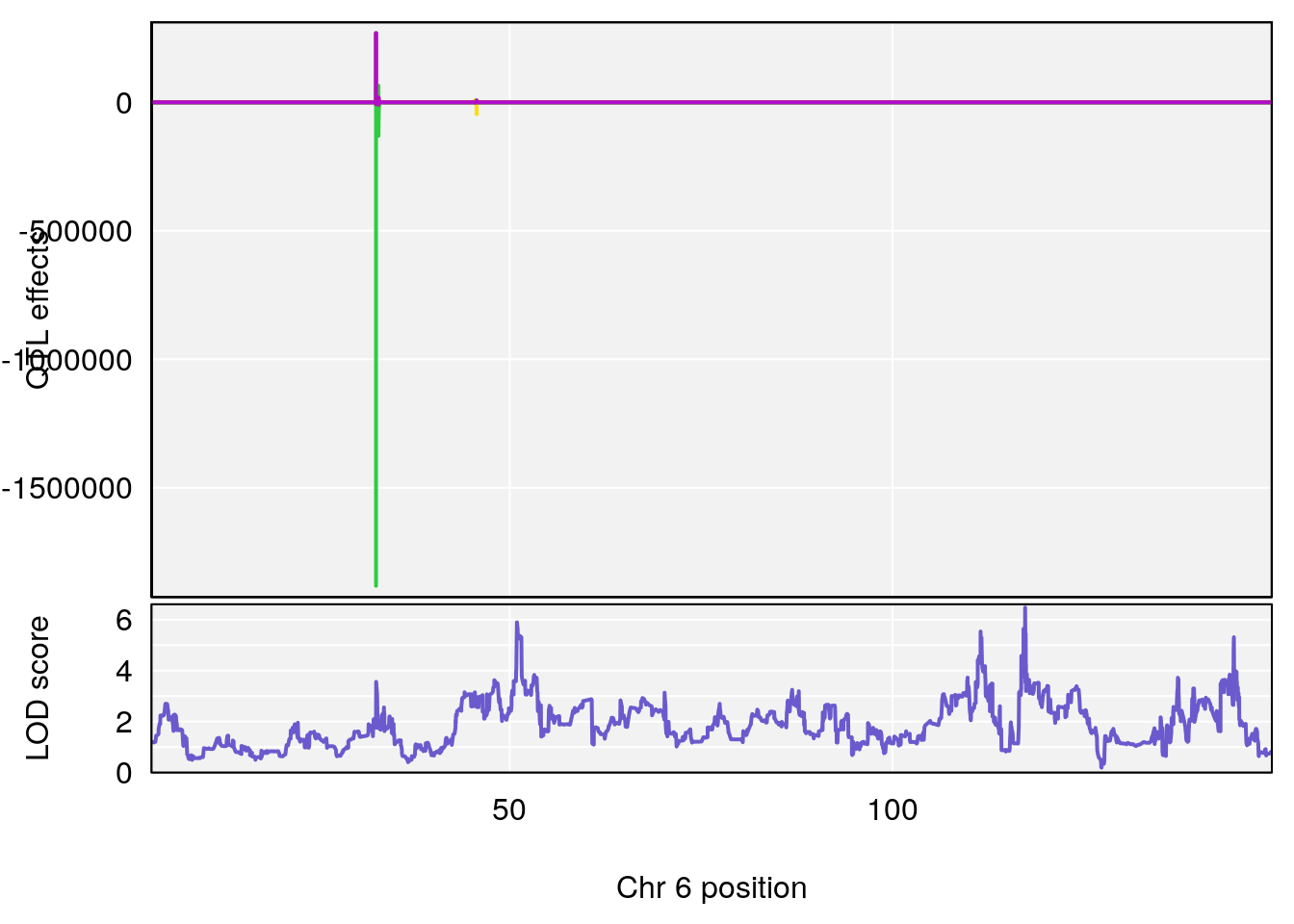
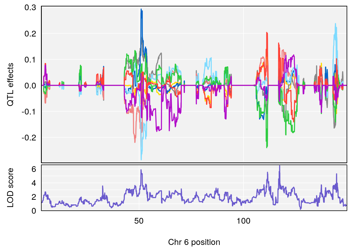
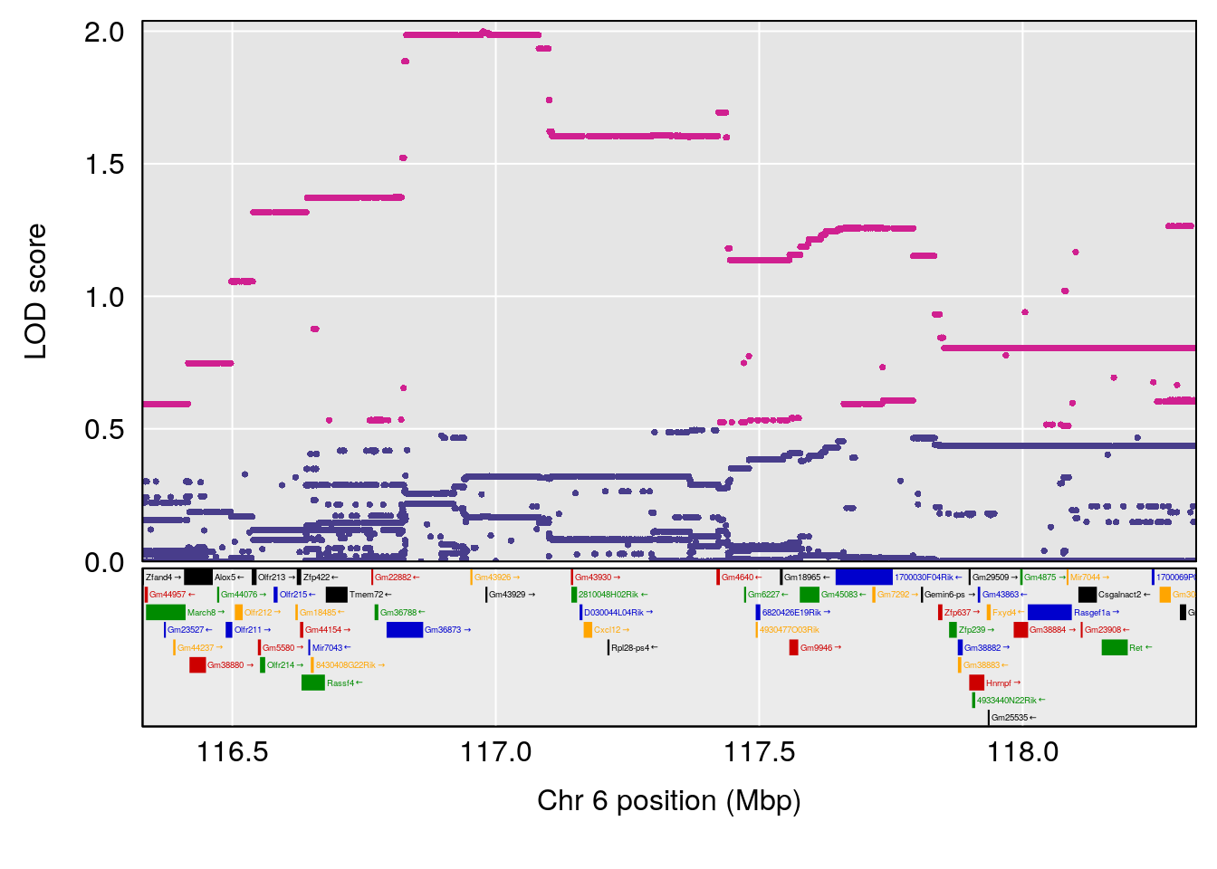
# [1] 4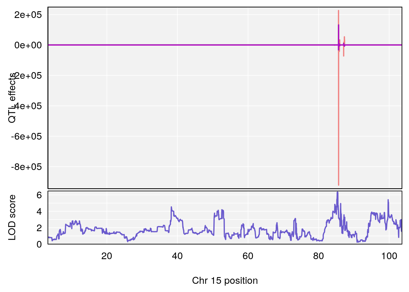
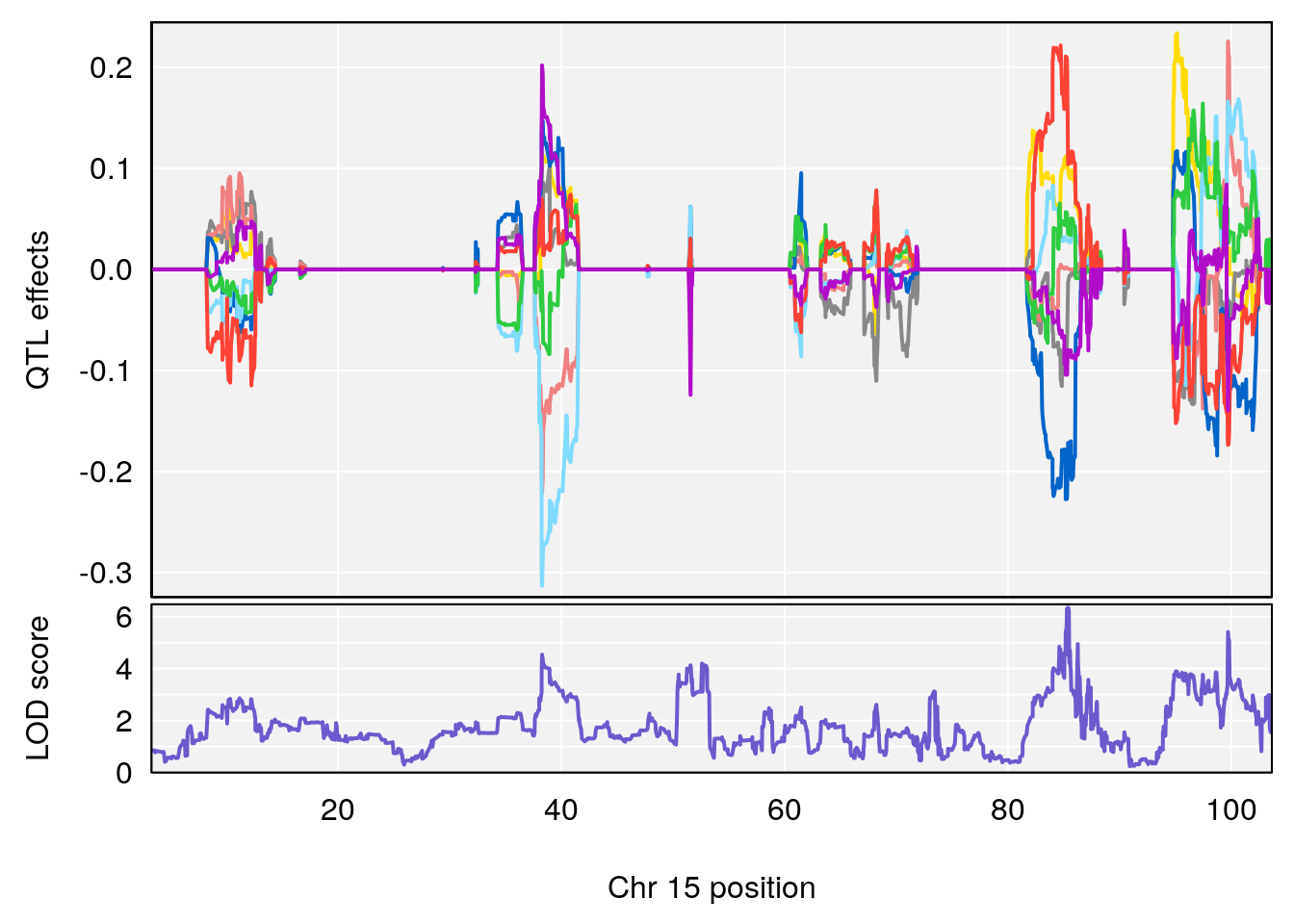
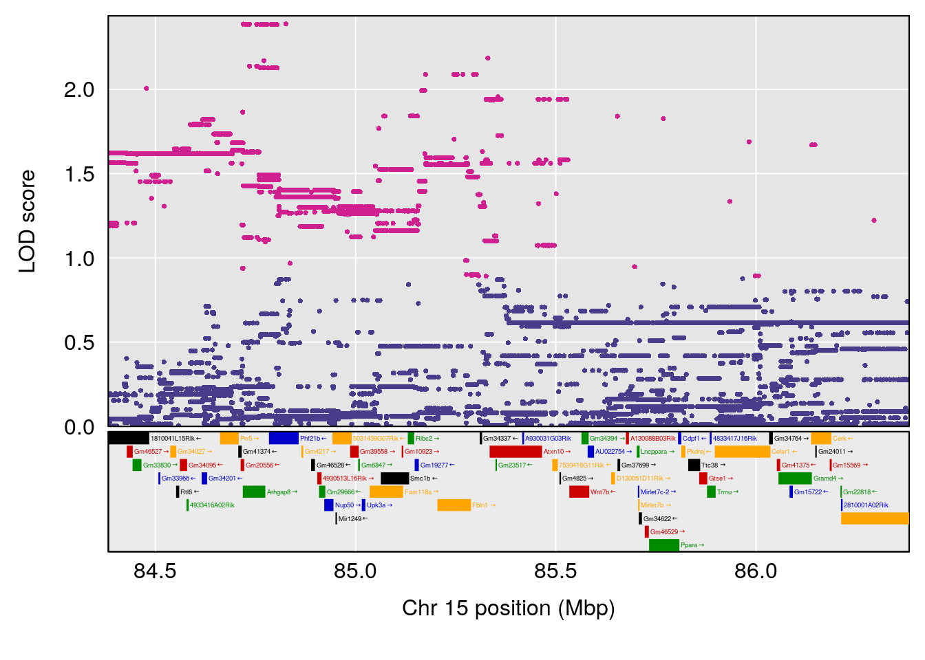
# [1] 5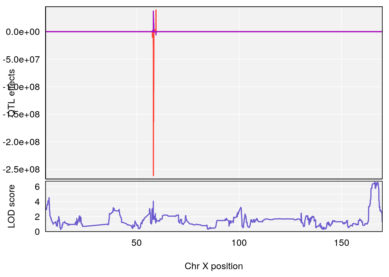
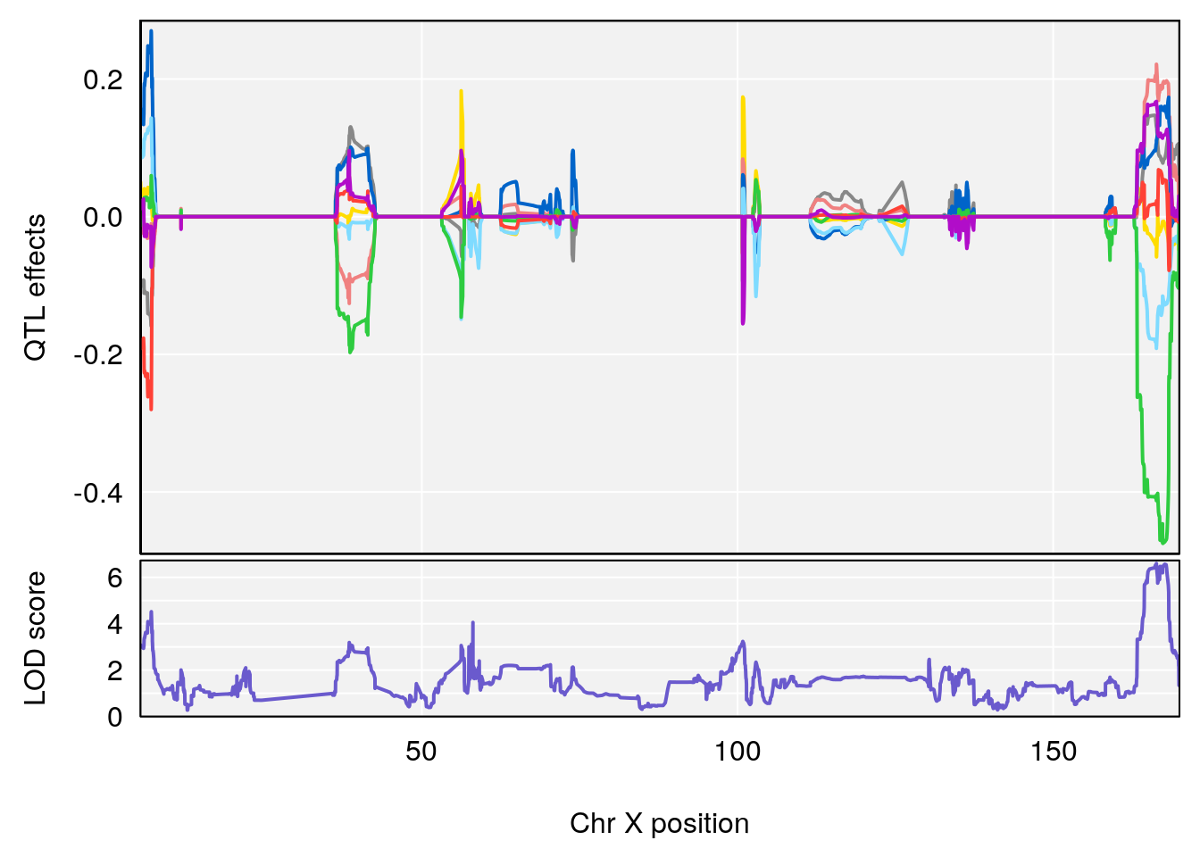
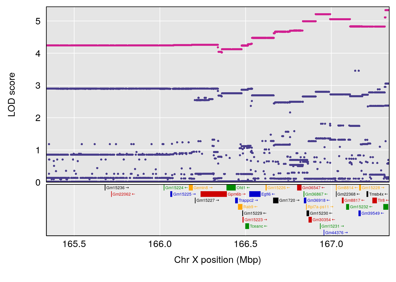
# [1] "f__Bpm"
#   lodindex lodcolumn chr      pos      lod    ci_lo   ci_hi
# 1        1    pheno1  19 11.00207 6.248255 10.75352 11.3772
# [1] 1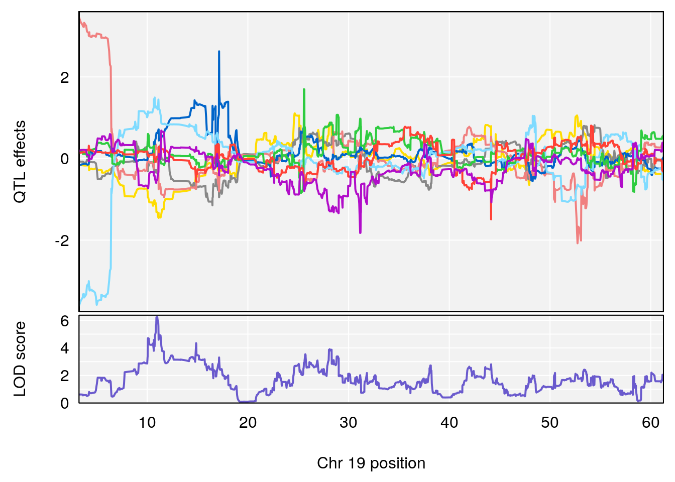
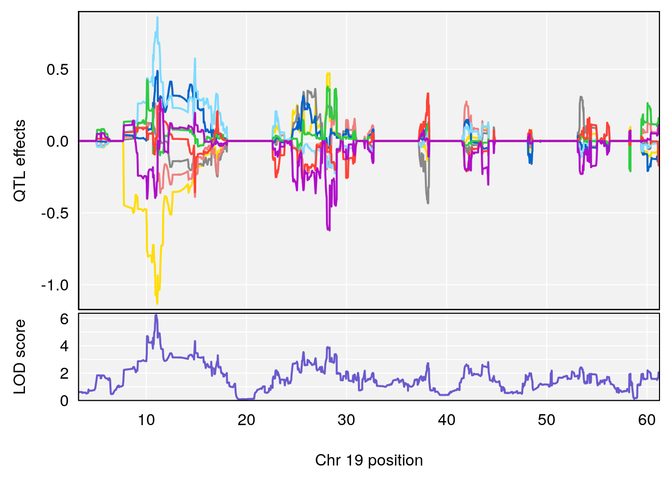
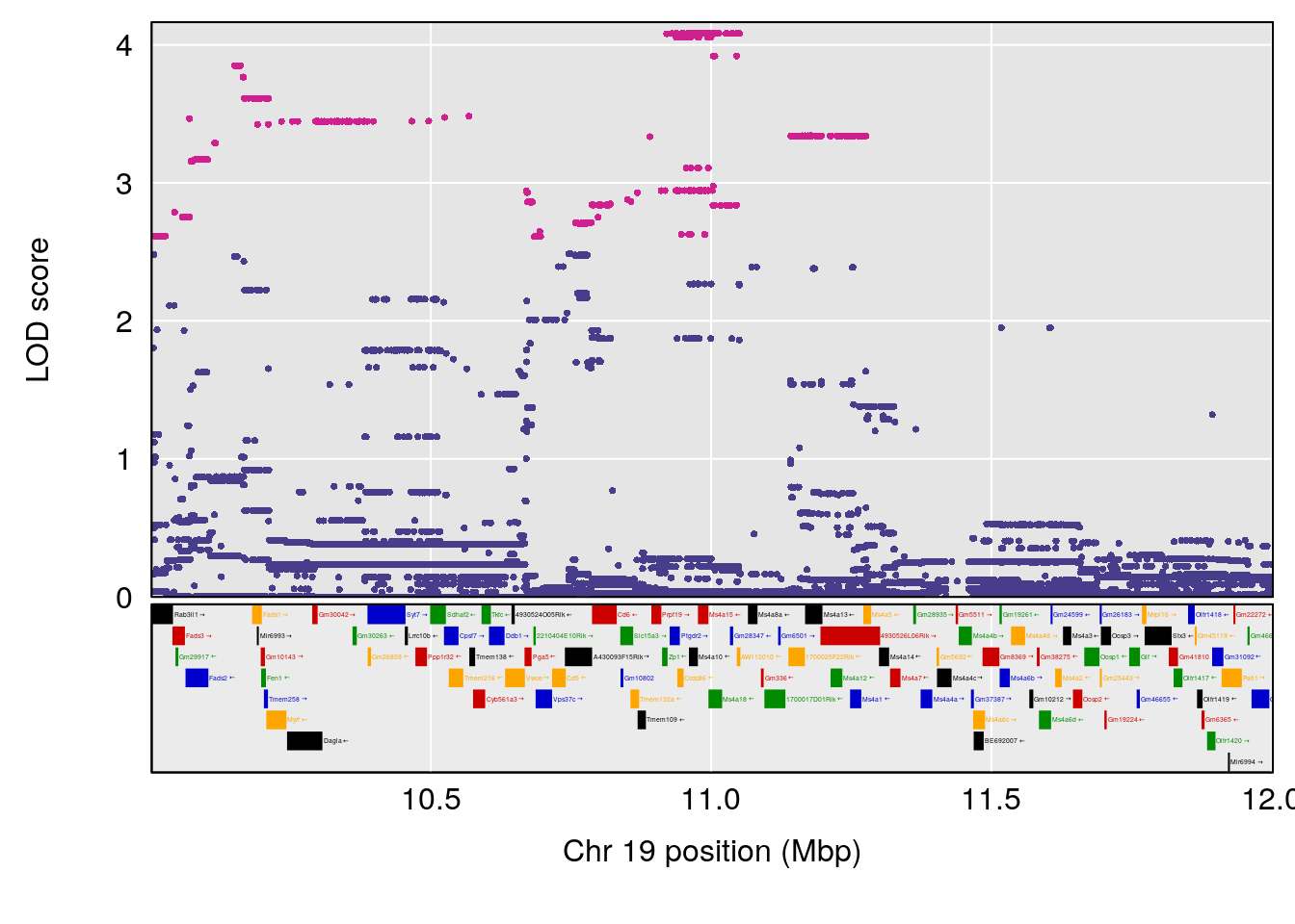
# [1] "TVb_ml"
#   lodindex lodcolumn chr       pos      lod     ci_lo     ci_hi
# 1        1    pheno1   1  30.63460 6.511425  25.52677  31.08521
# 2        1    pheno1  10 122.95839 6.485486 122.24637 123.28591
# 3        1    pheno1  18  47.44584 7.056038  46.97402  49.46217
# [1] 1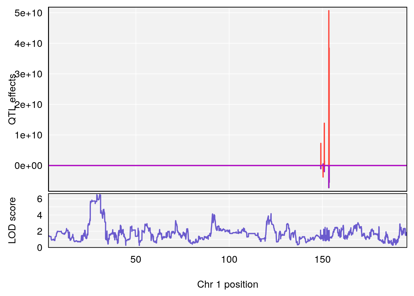
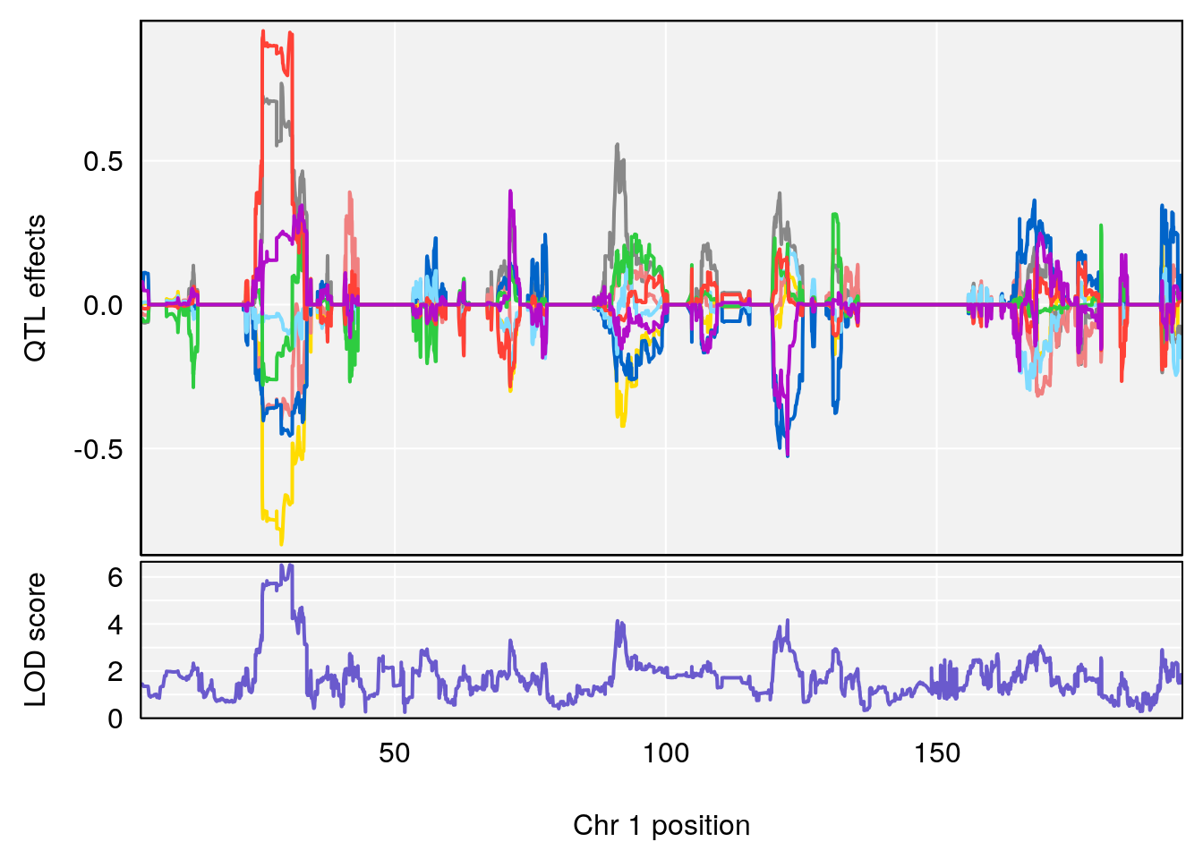
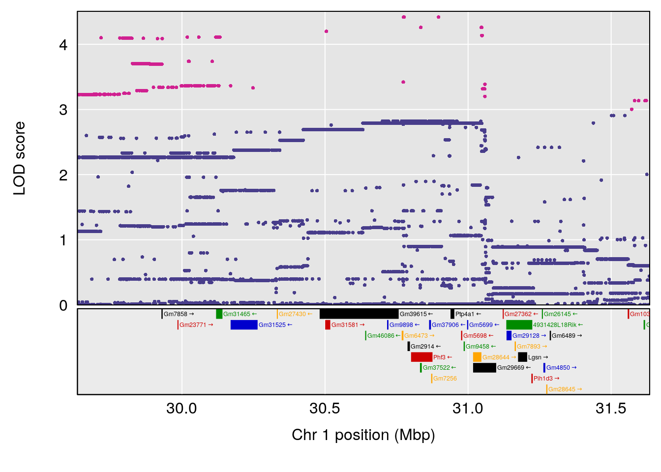
# [1] 2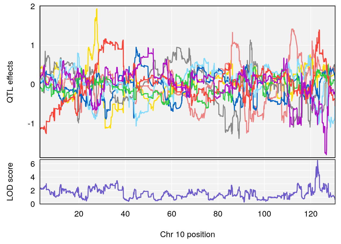
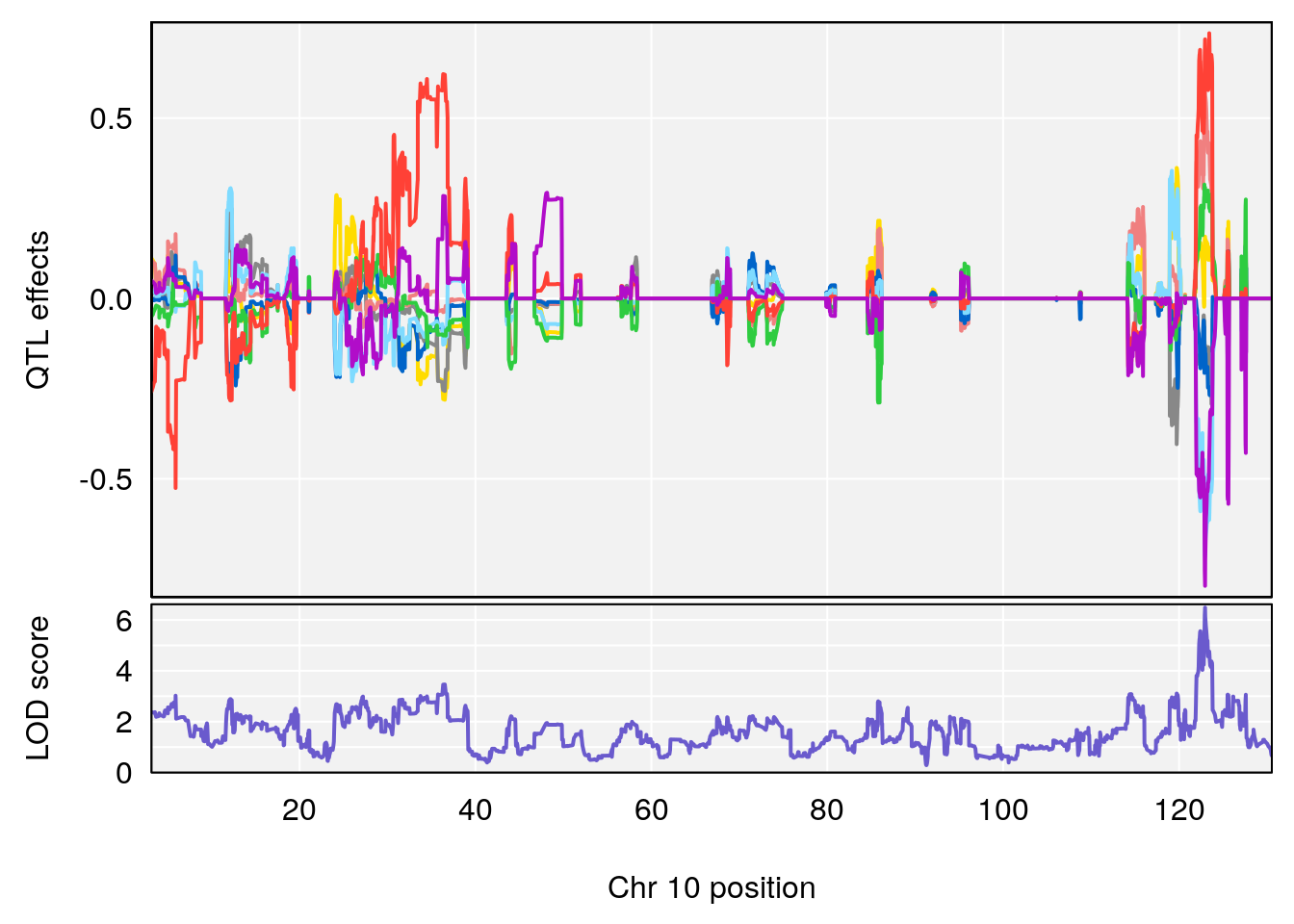
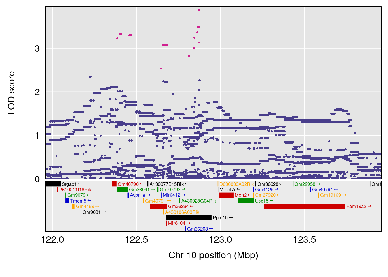
# [1] 3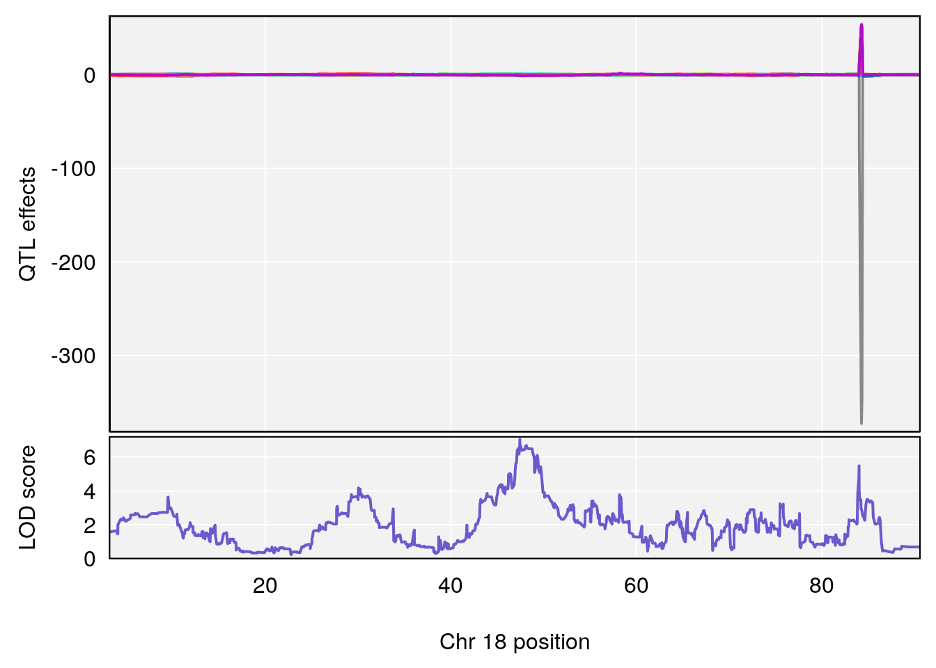
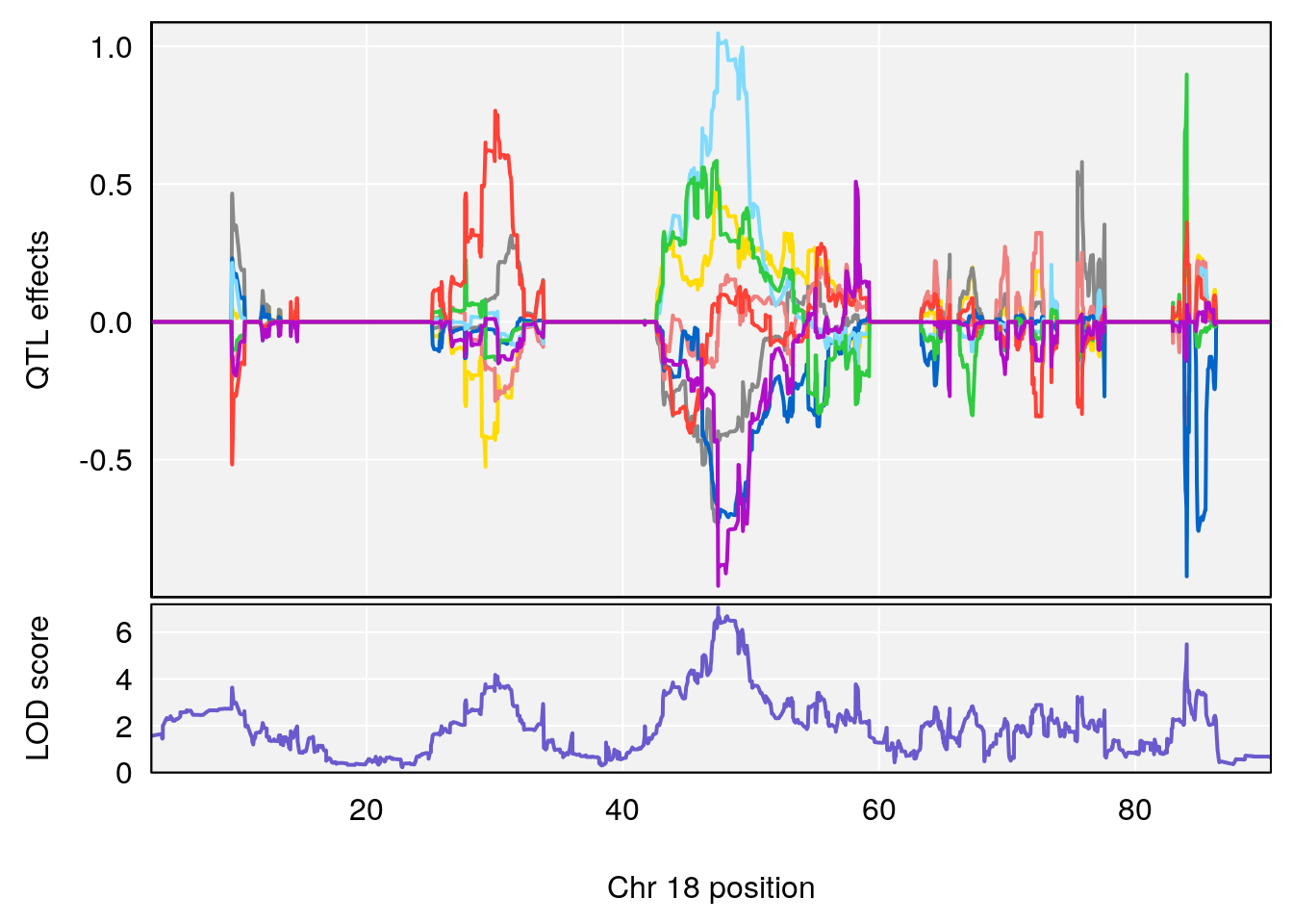
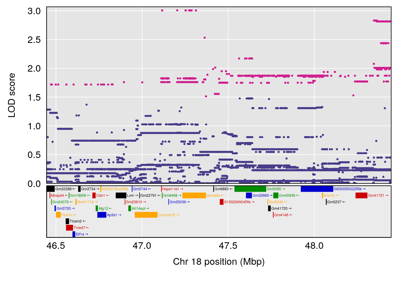
# [1] "MVb__ml_min"
# [1] lodindex  lodcolumn chr       pos       lod       ci_lo     ci_hi
# <0 rows> (or 0-length row.names)
# [1] "Penh"
#   lodindex lodcolumn chr       pos      lod     ci_lo     ci_hi
# 1        1    pheno1   3 128.34723 7.161796 105.50059 128.70283
# 2        1    pheno1   9 105.09628 6.694530 104.93950 108.96924
# 3        1    pheno1  11  44.63764 6.061567  44.01853  45.57241
# [1] 1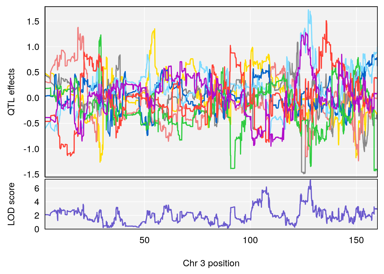
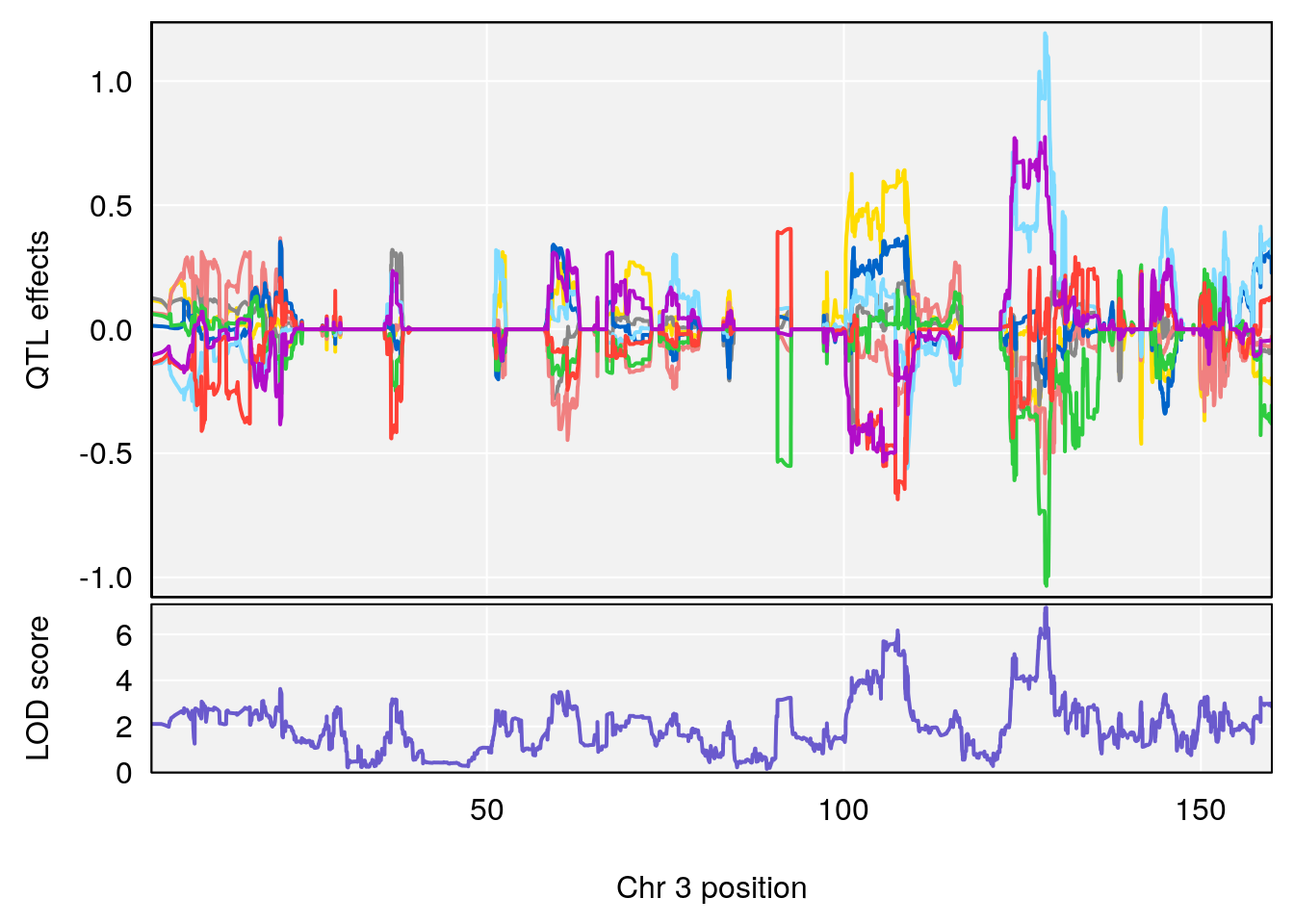
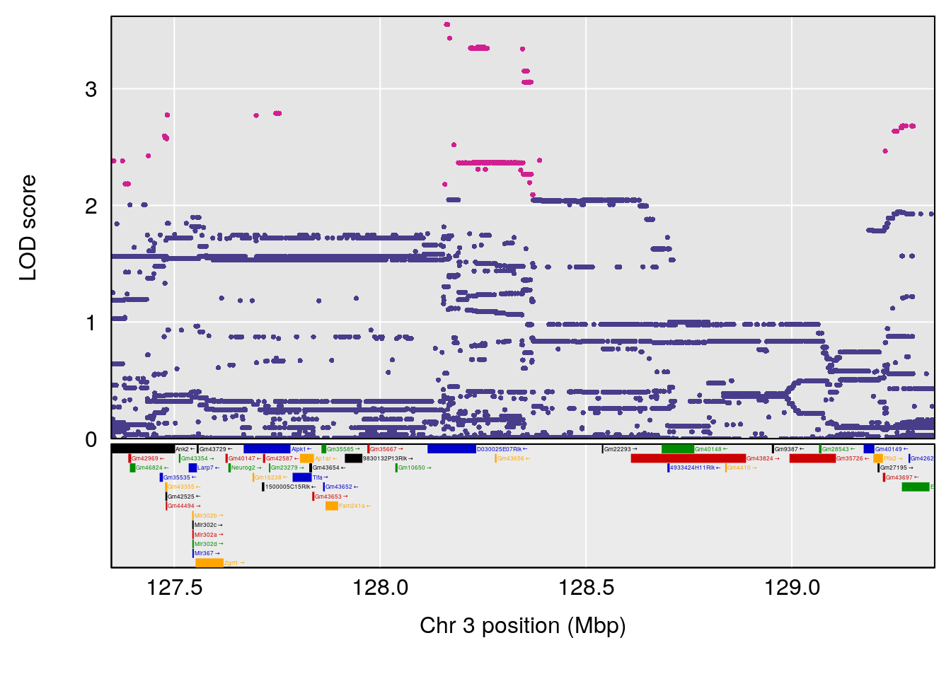
# [1] 2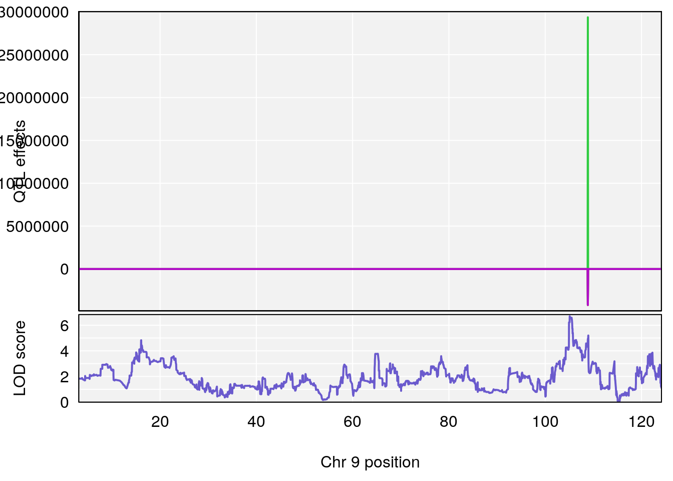
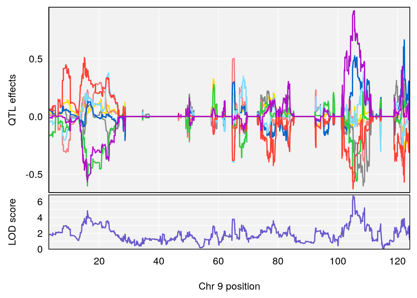
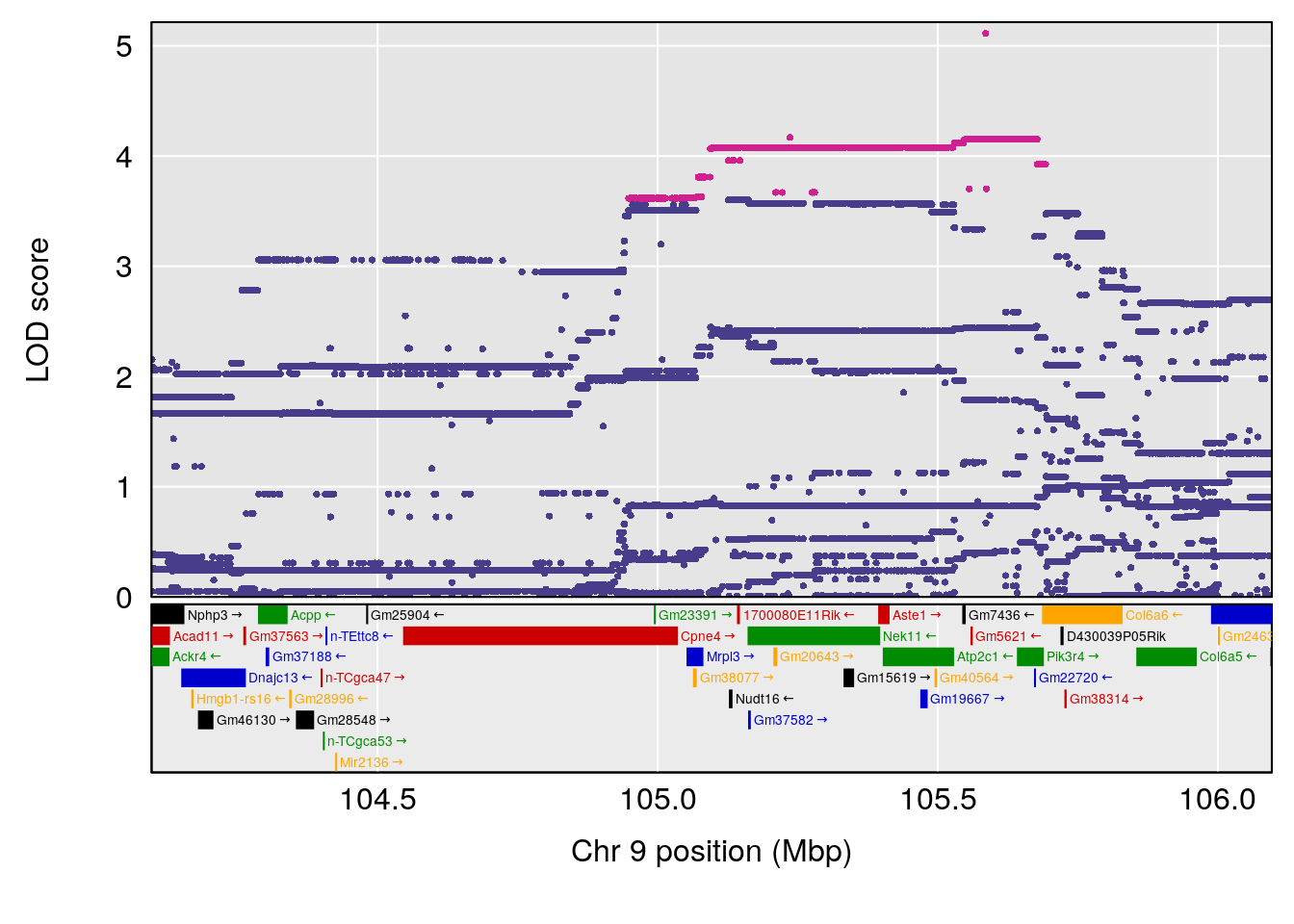
# [1] 3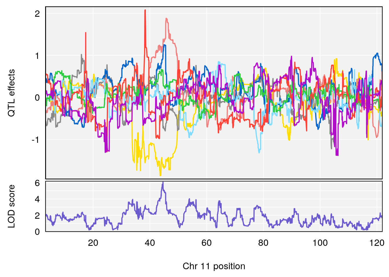
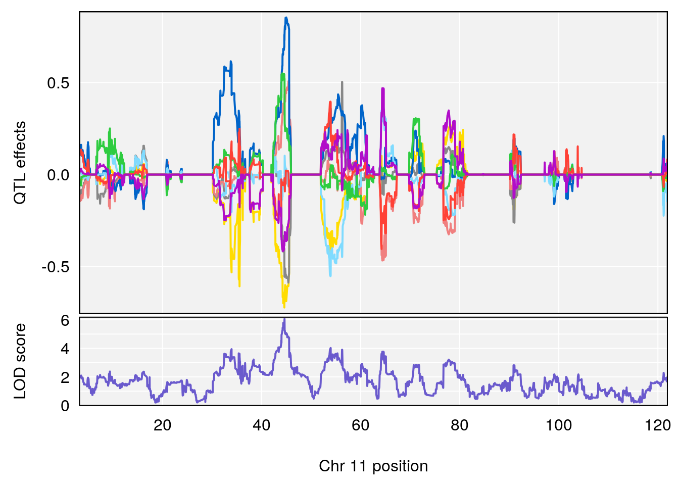
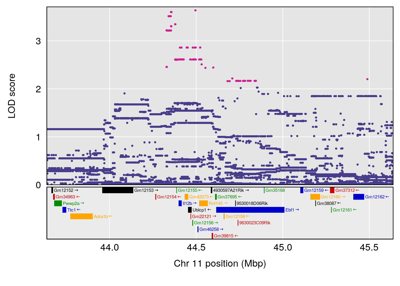
# [1] "PAU"
#   lodindex lodcolumn chr       pos      lod     ci_lo     ci_hi
# 1        1    pheno1   9 105.16275 6.947873 104.93950 106.42138
# 2        1    pheno1  11  44.63764 6.932076  44.01853  45.57241
# [1] 1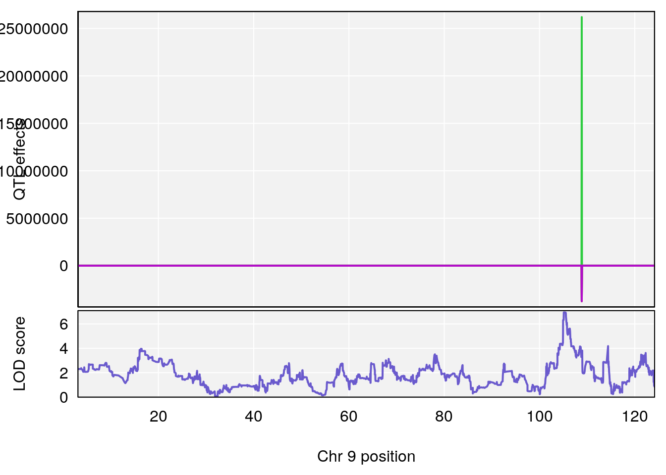
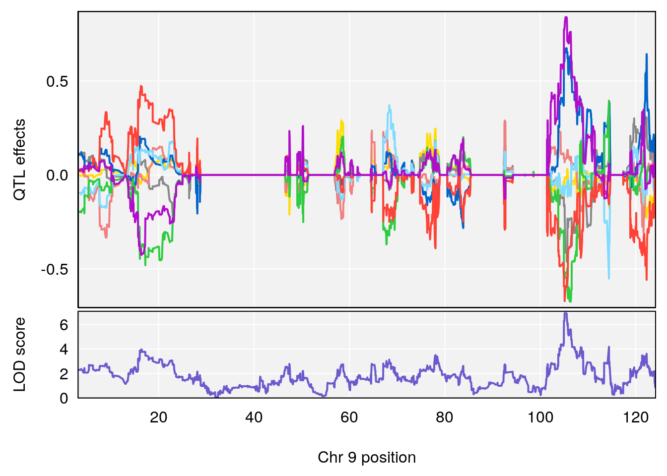
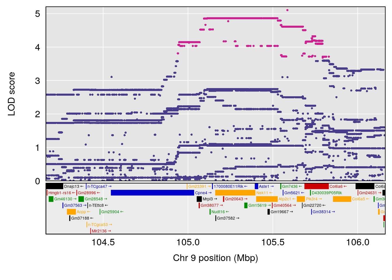
# [1] 2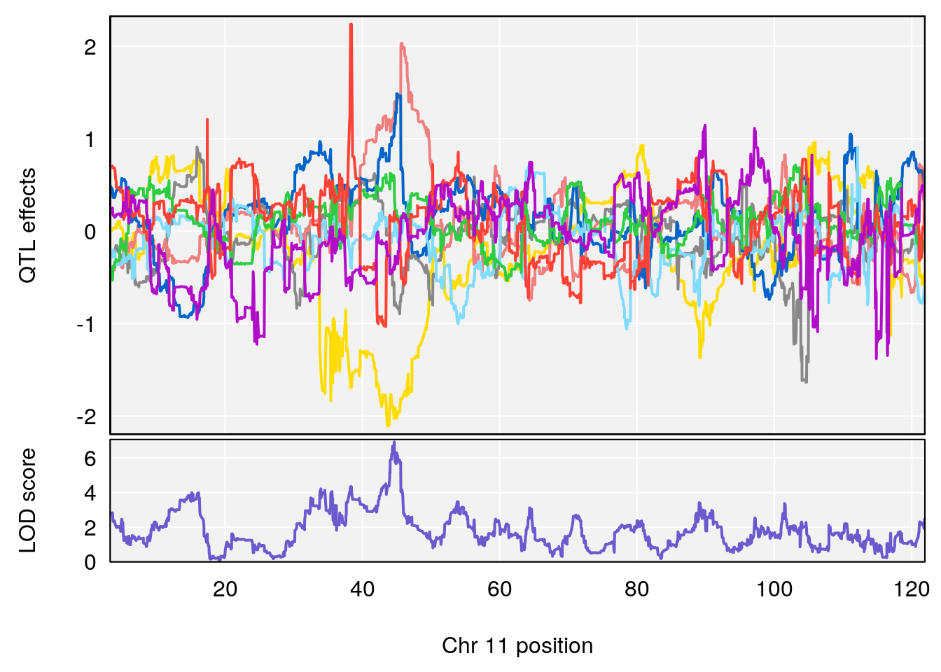
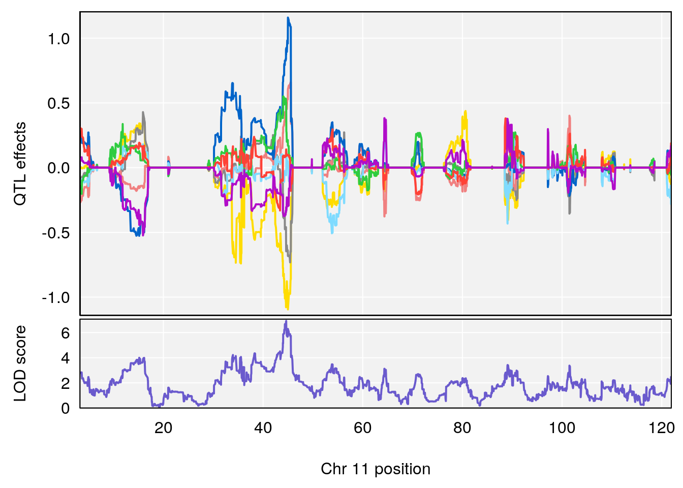
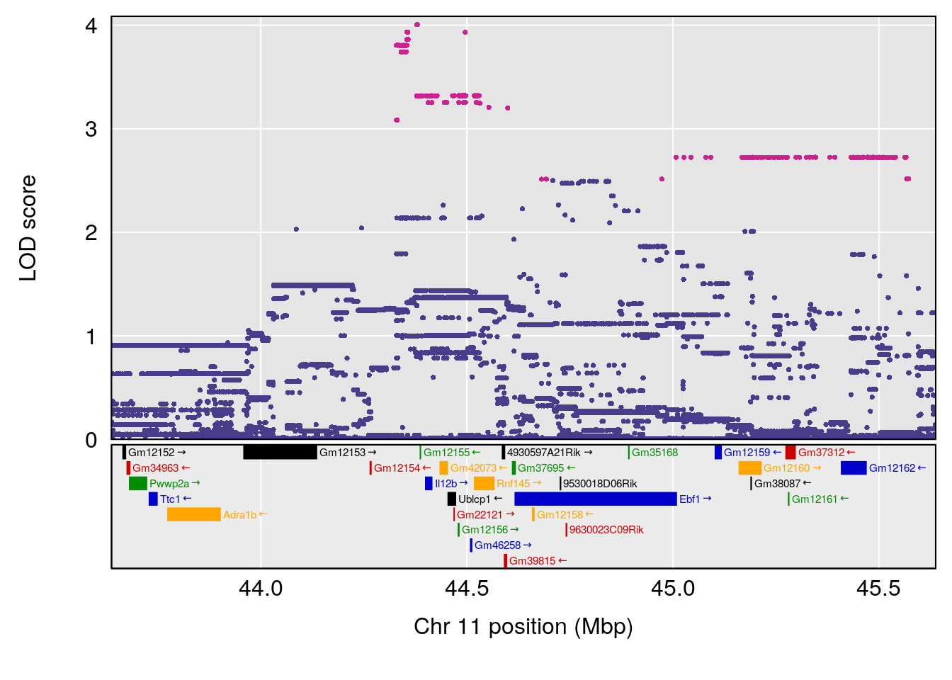
# [1] "Rpef"
#   lodindex lodcolumn chr       pos      lod    ci_lo     ci_hi
# 1        1    pheno1   3 103.29787 6.430433 97.19254 104.52824
# 2        1    pheno1  11  45.41904 6.048635 44.22489  45.59516
# 3        1    pheno1   X  47.58251 6.184616 45.33643  47.96484
# [1] 1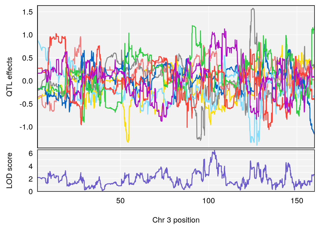
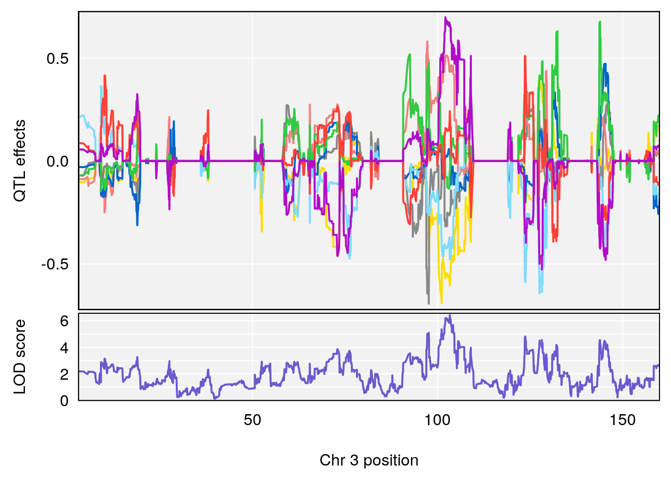
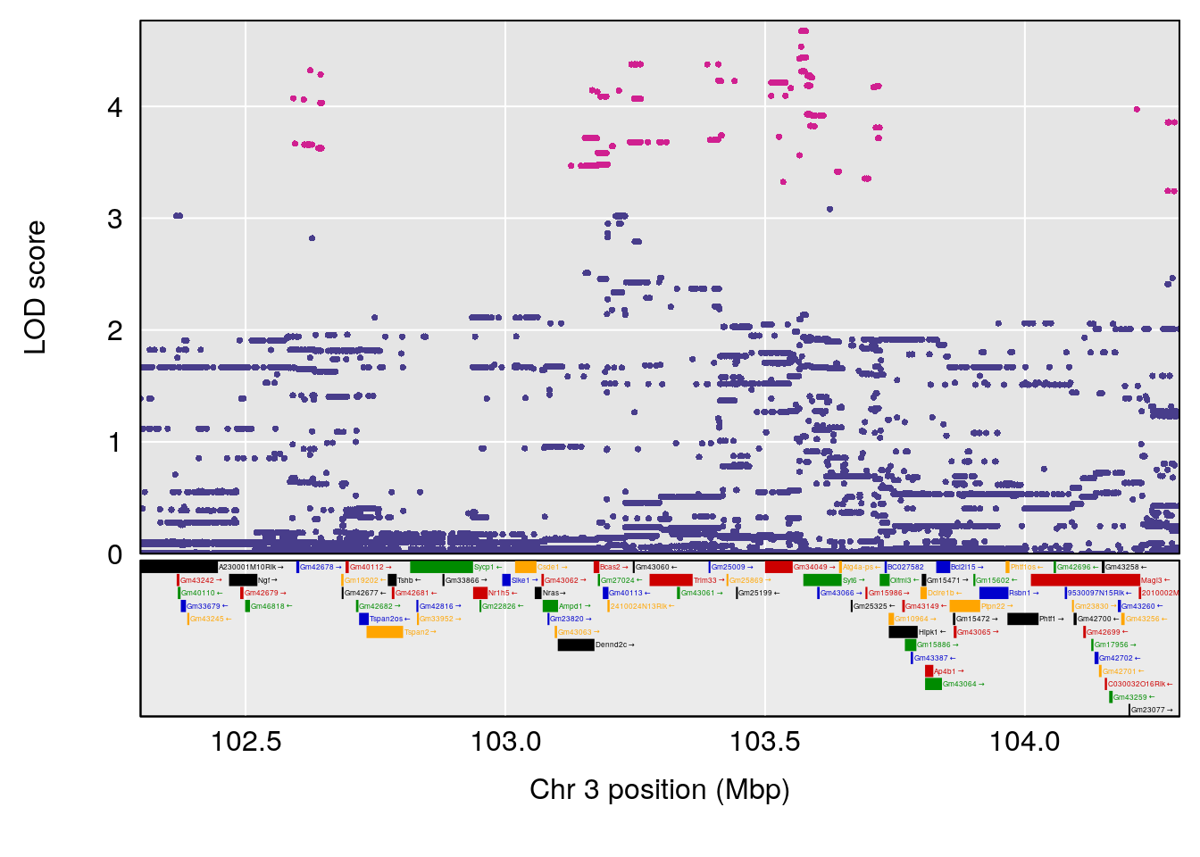
# [1] 2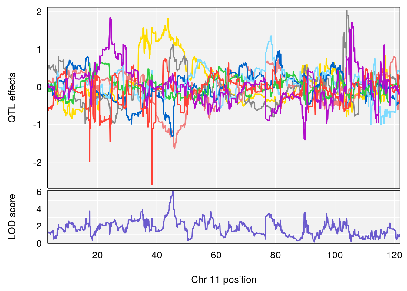
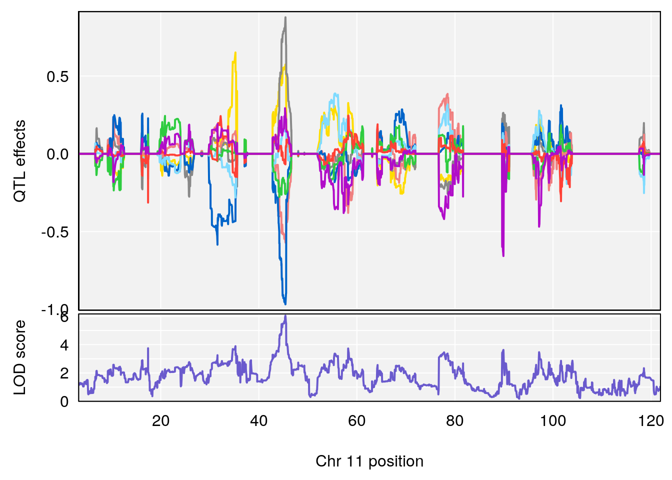
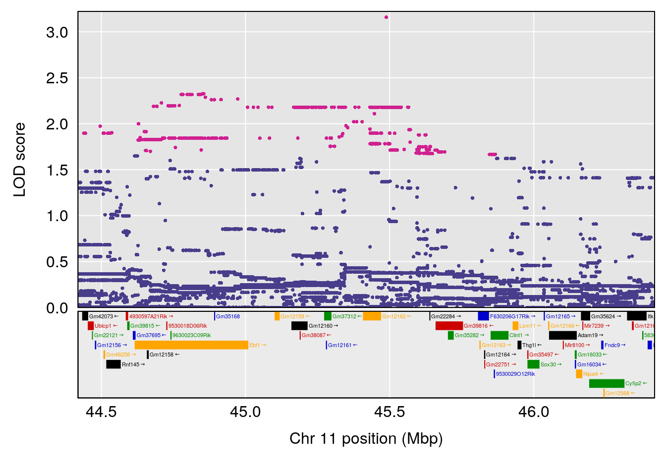
# [1] 3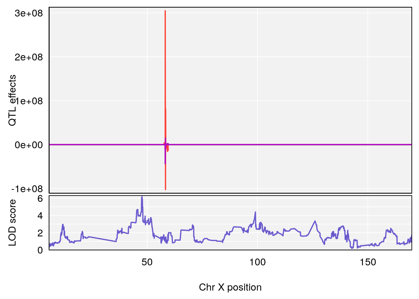
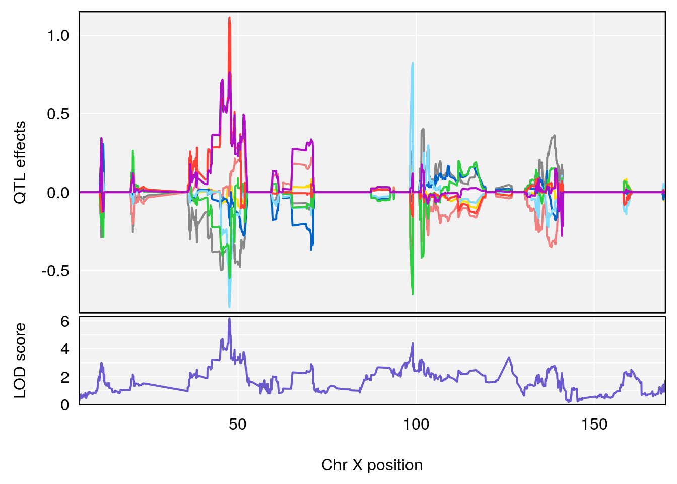
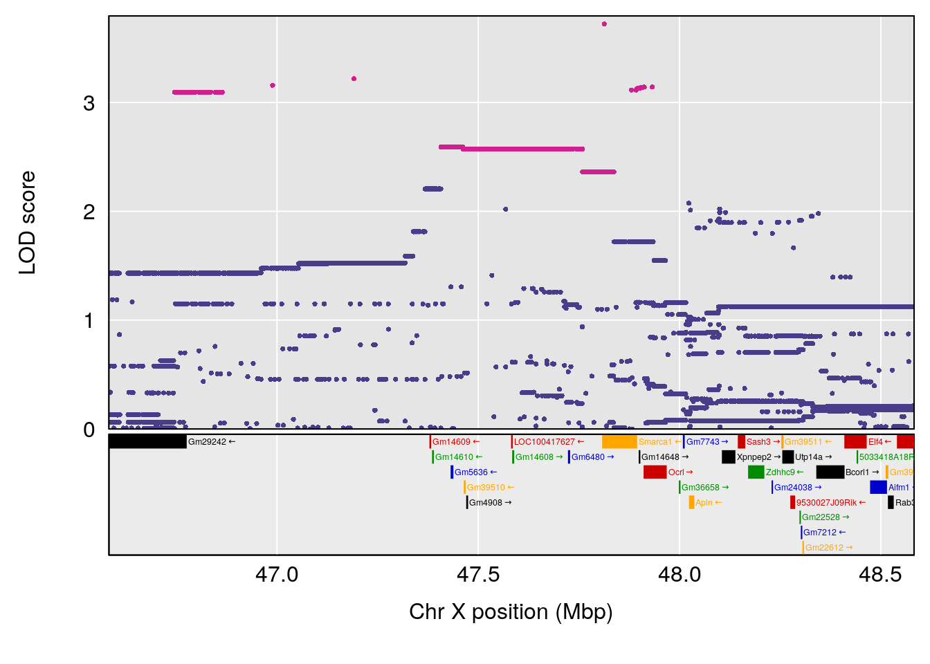
# [1] "PIFb"
#   lodindex lodcolumn chr      pos      lod    ci_lo    ci_hi
# 1        1    pheno1  12 16.00241 6.053423 15.85922 89.14611
# [1] 1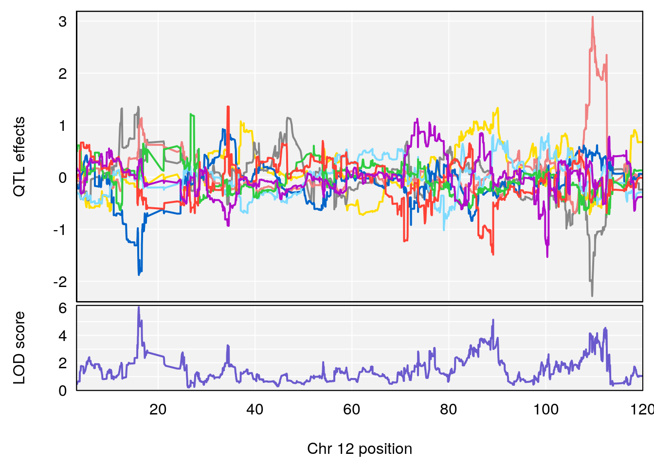
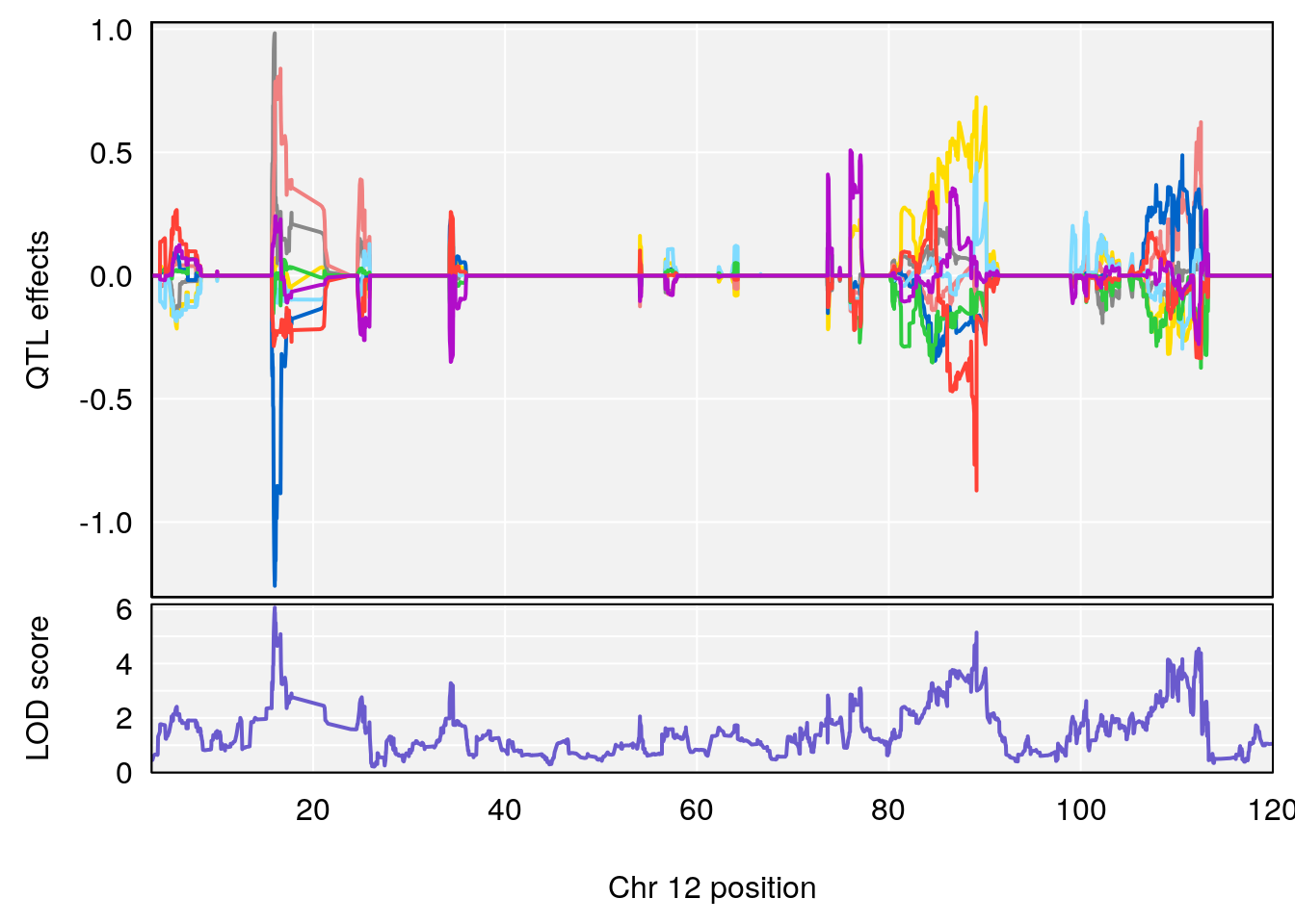
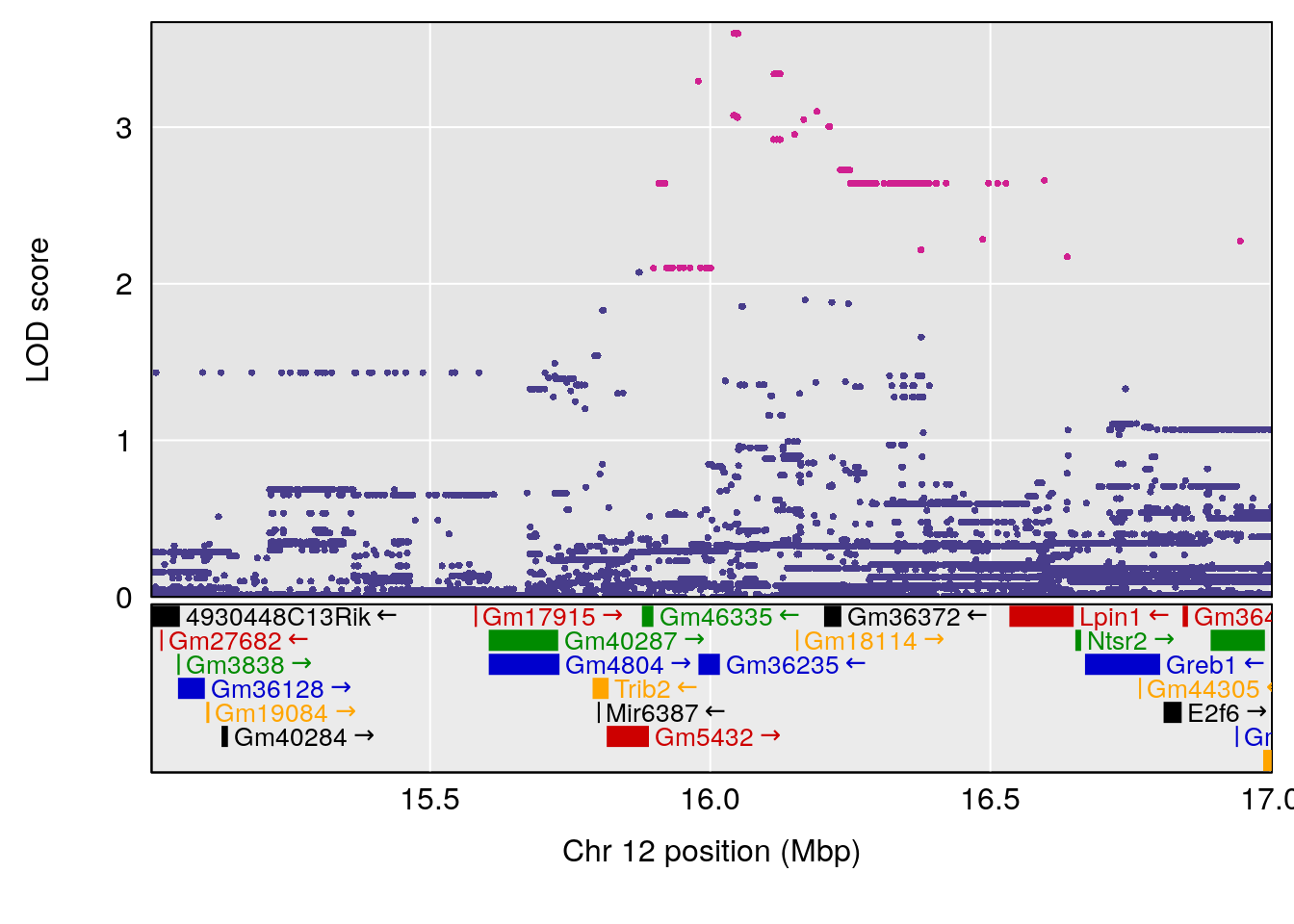
# [1] "PEFb"
# [1] lodindex  lodcolumn chr       pos       lod       ci_lo     ci_hi
# <0 rows> (or 0-length row.names)
# [1] "Ti__sec"
#   lodindex lodcolumn chr      pos      lod    ci_lo    ci_hi
# 1        1    pheno1  12 16.00241 6.810402 15.89116 112.6024
# [1] 1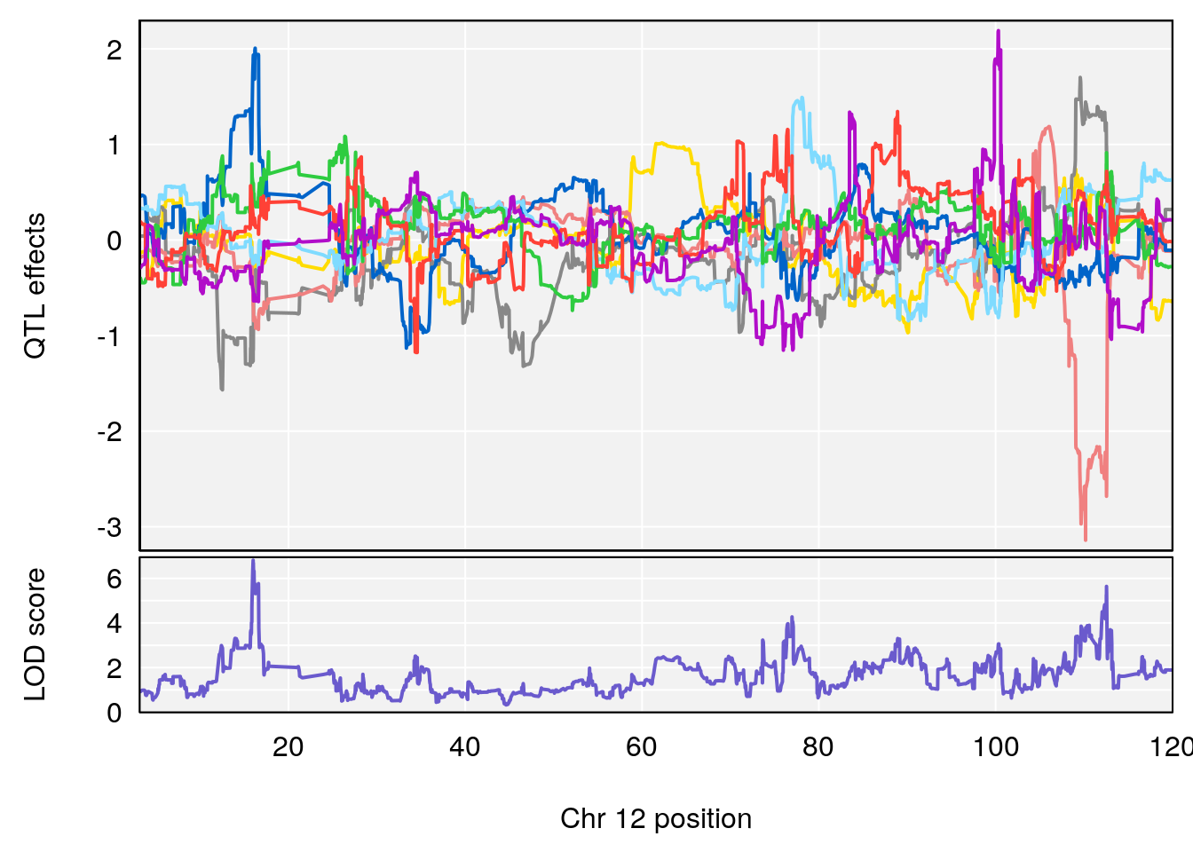
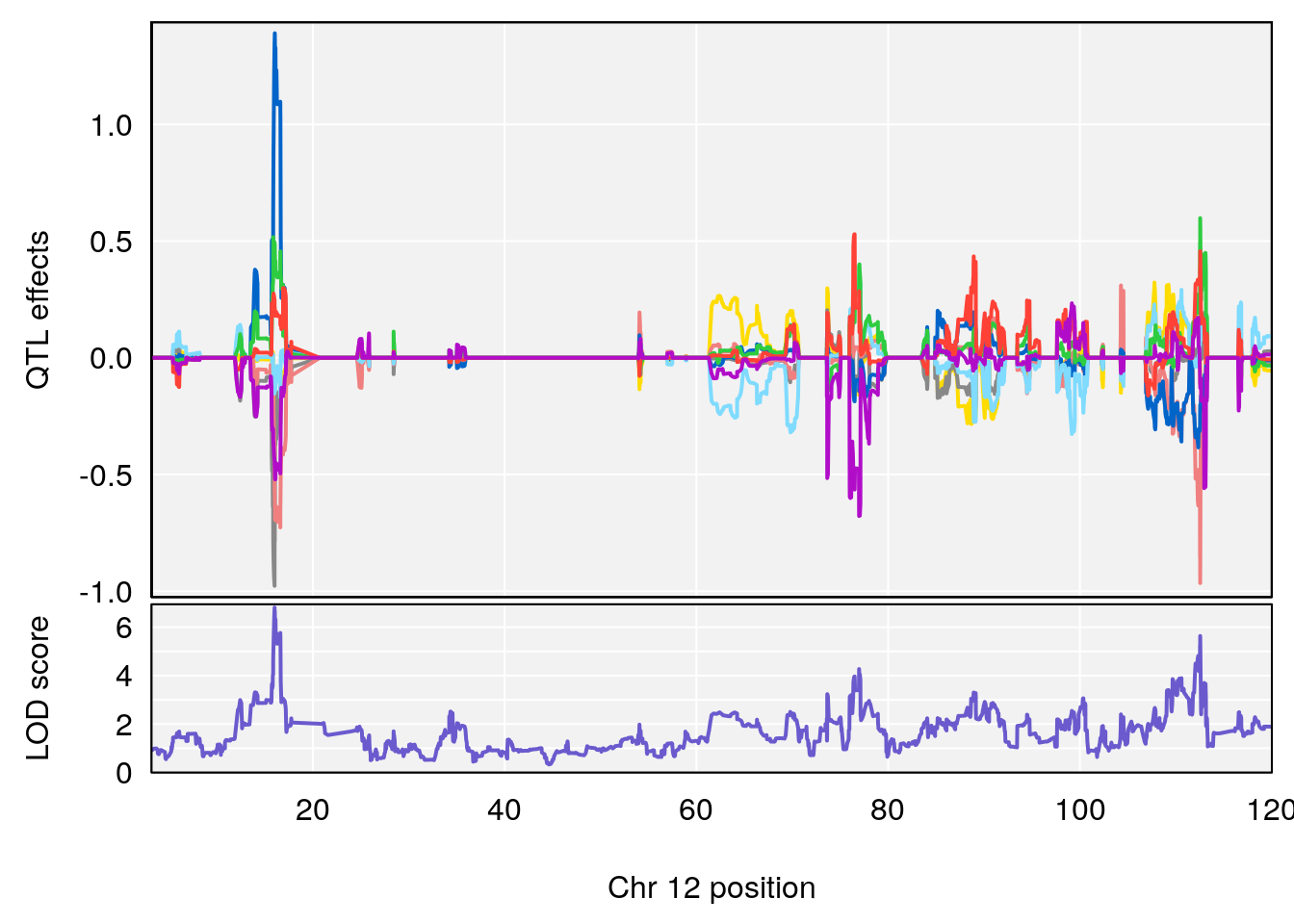
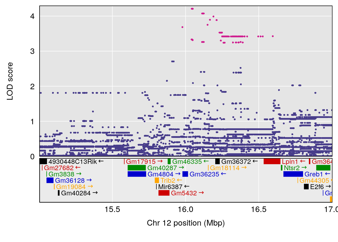
# [1] "Te__sec"
#   lodindex lodcolumn chr      pos      lod    ci_lo    ci_hi
# 1        1    pheno1  19 10.10562 6.523658 10.05116 14.88277
# 2        1    pheno1   X 47.58251 6.615726 47.33842 48.09622
# [1] 1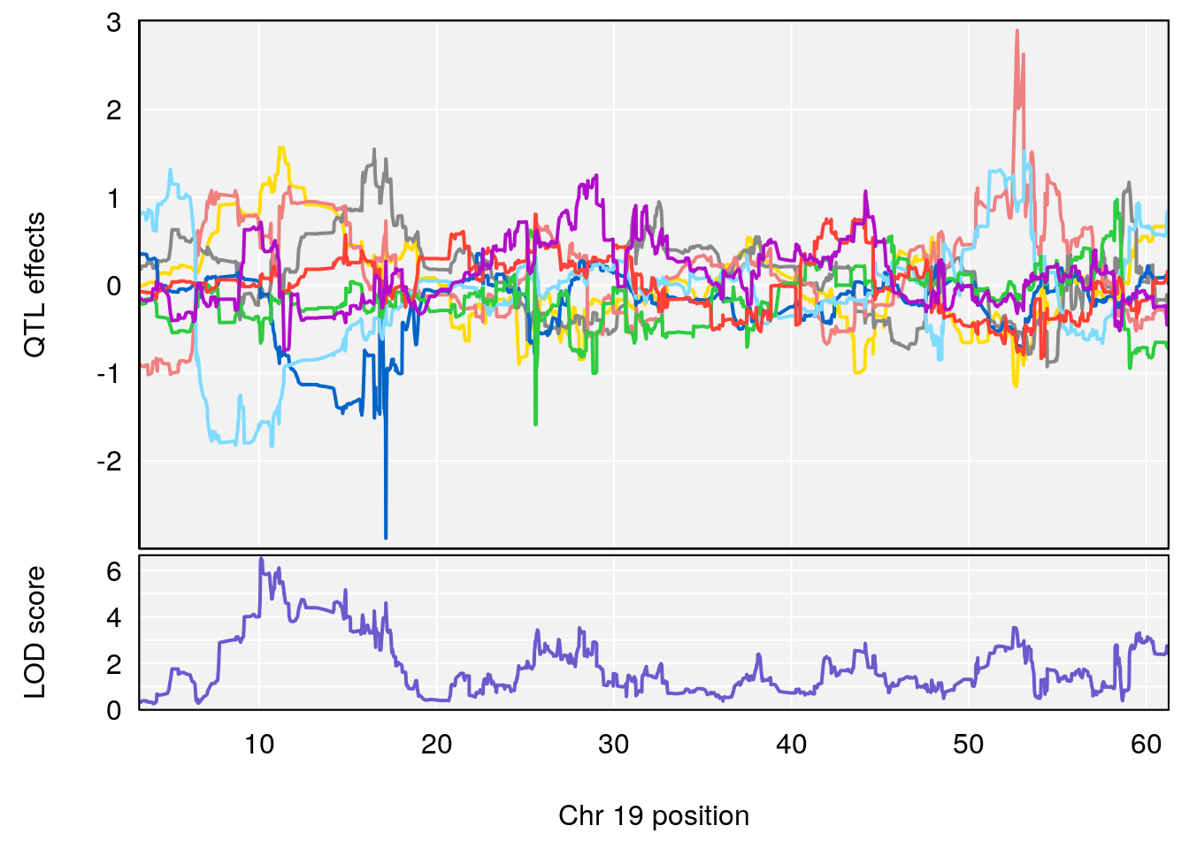
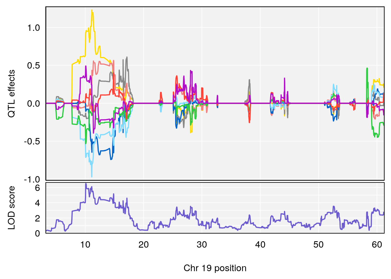
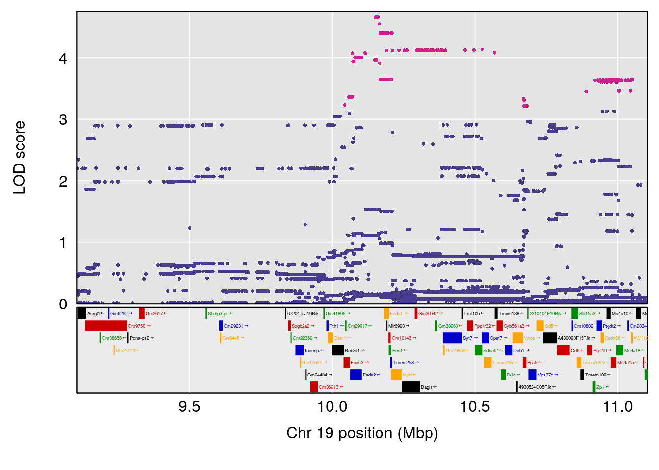
# [1] 2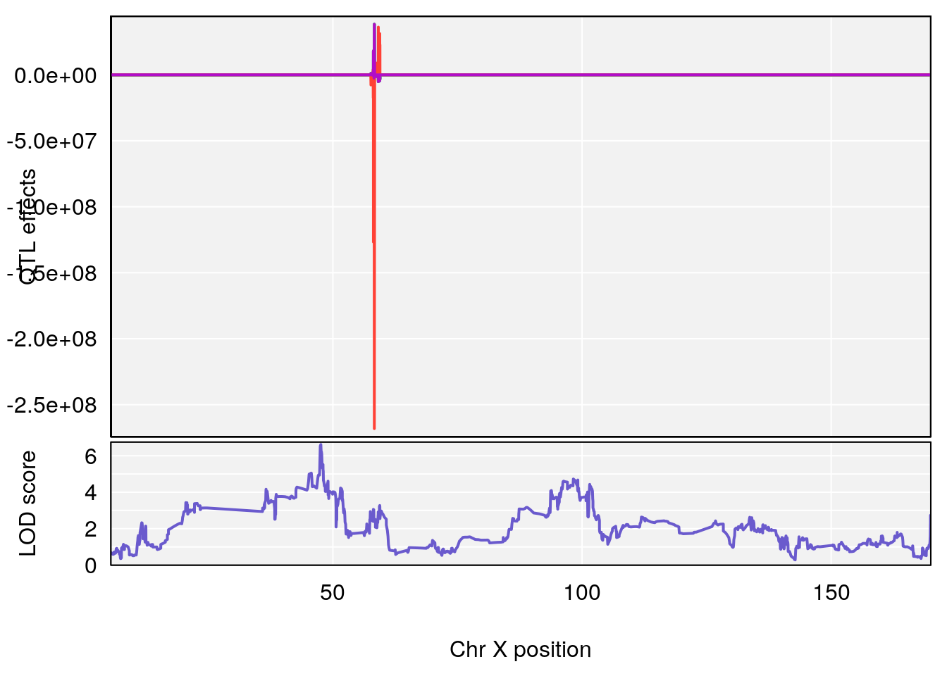
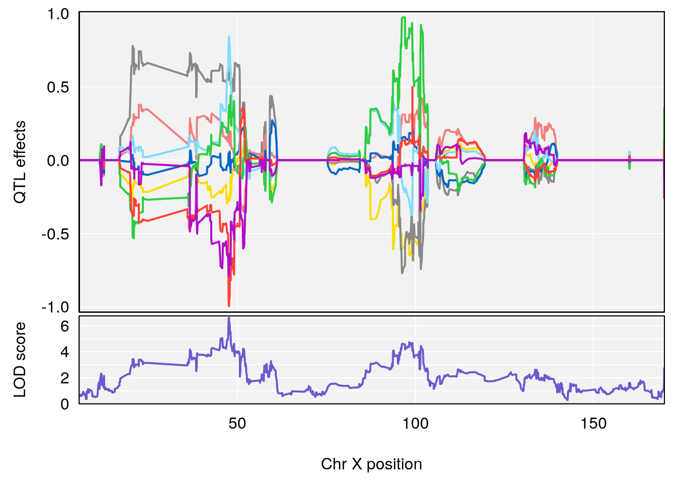
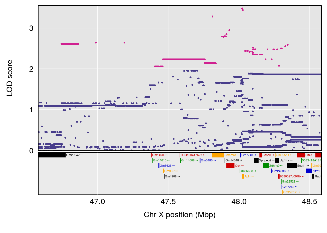
# [1] "EF50"
# [1] lodindex  lodcolumn chr       pos       lod       ci_lo     ci_hi
# <0 rows> (or 0-length row.names)
# [1] "EIP__ms"
#   lodindex lodcolumn chr      pos       lod    ci_lo    ci_hi
# 1        1    pheno1   4 58.80643  6.364663 58.10783 59.46177
# 2        1    pheno1  19 12.38701 11.448067 11.68910 14.48196
# 3        1    pheno1   X 98.93218  8.113515 97.14698 99.11946
# [1] 1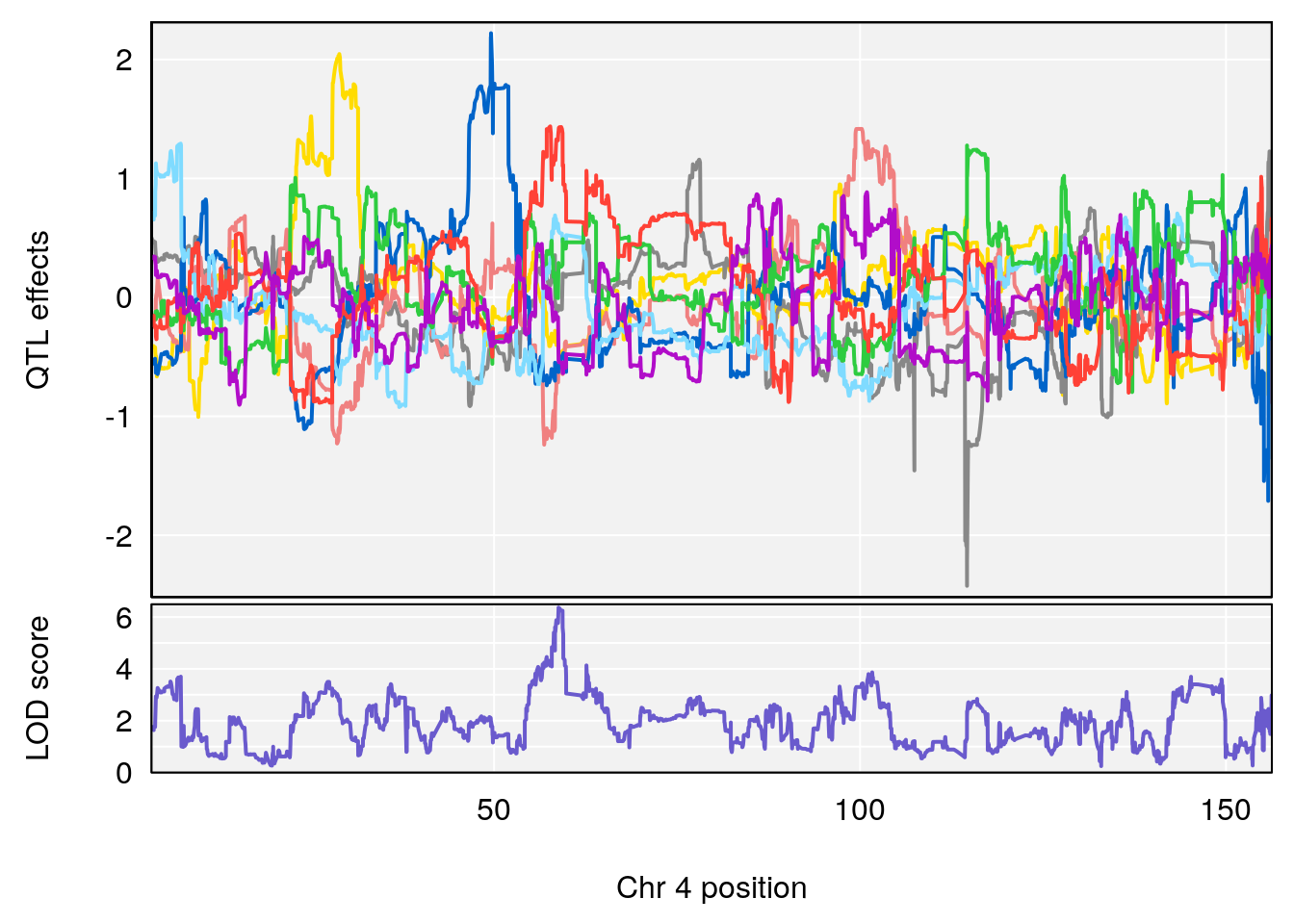
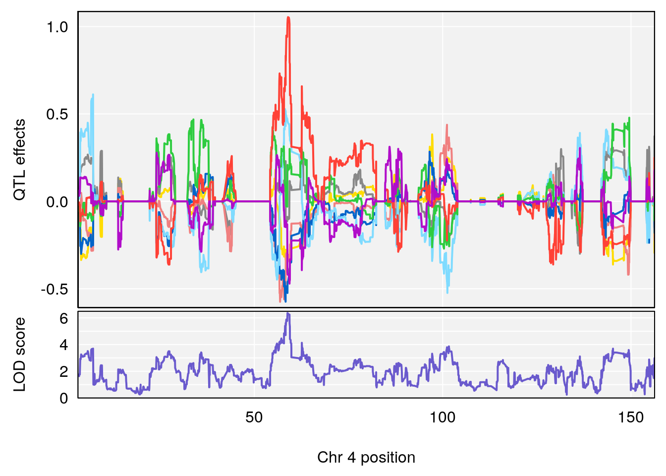
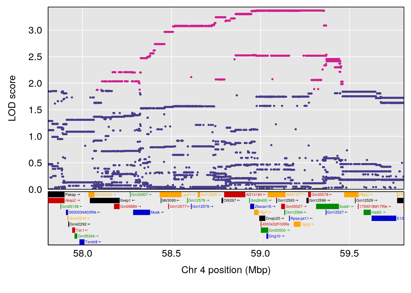
# [1] 2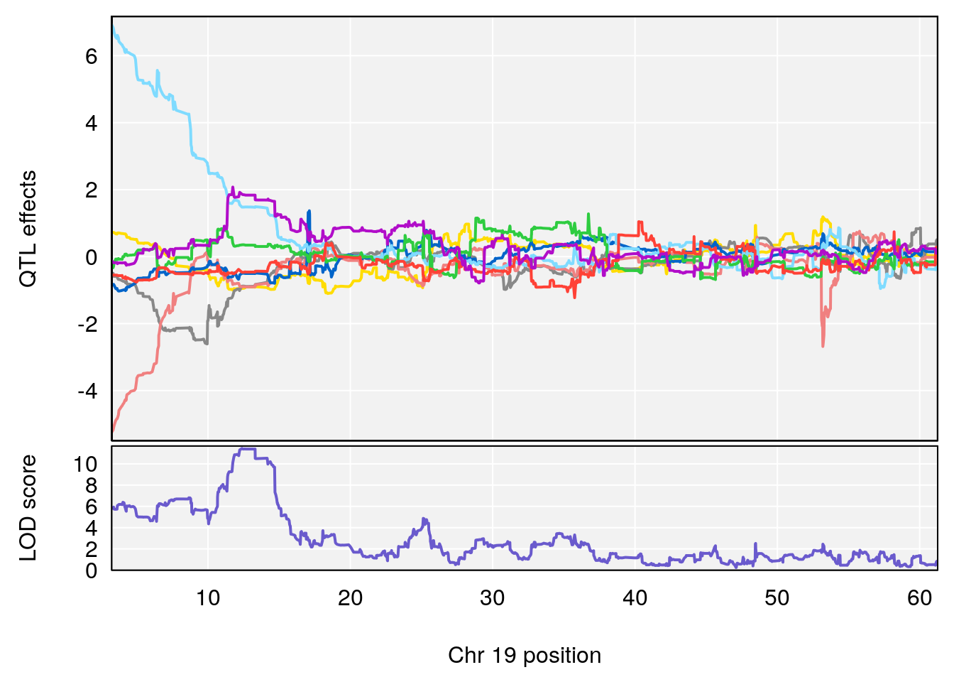
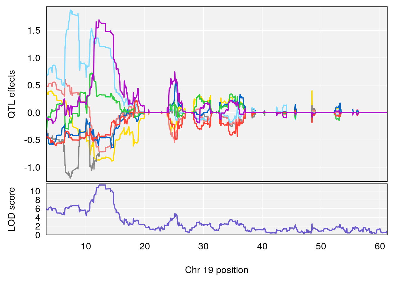
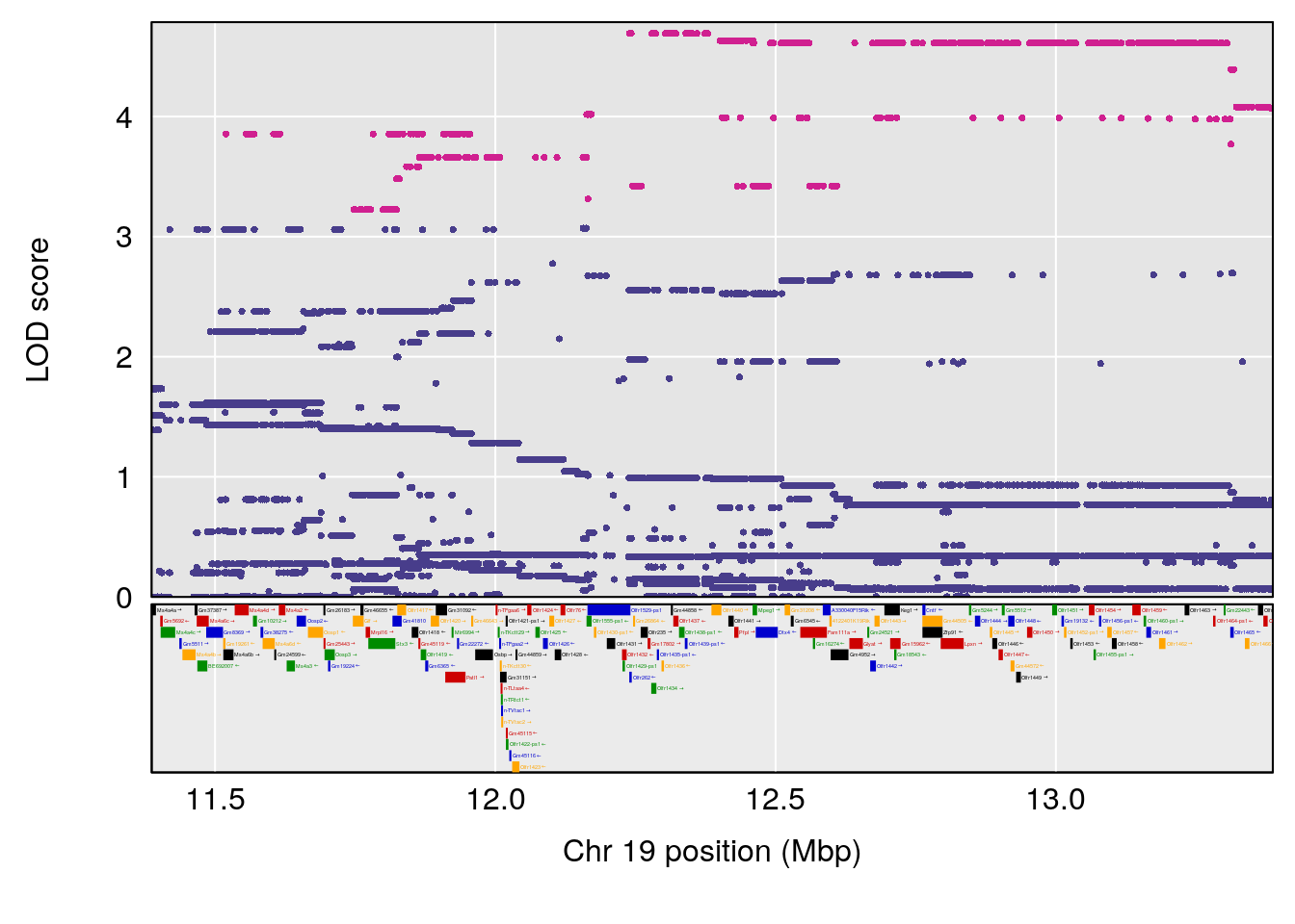
# [1] 3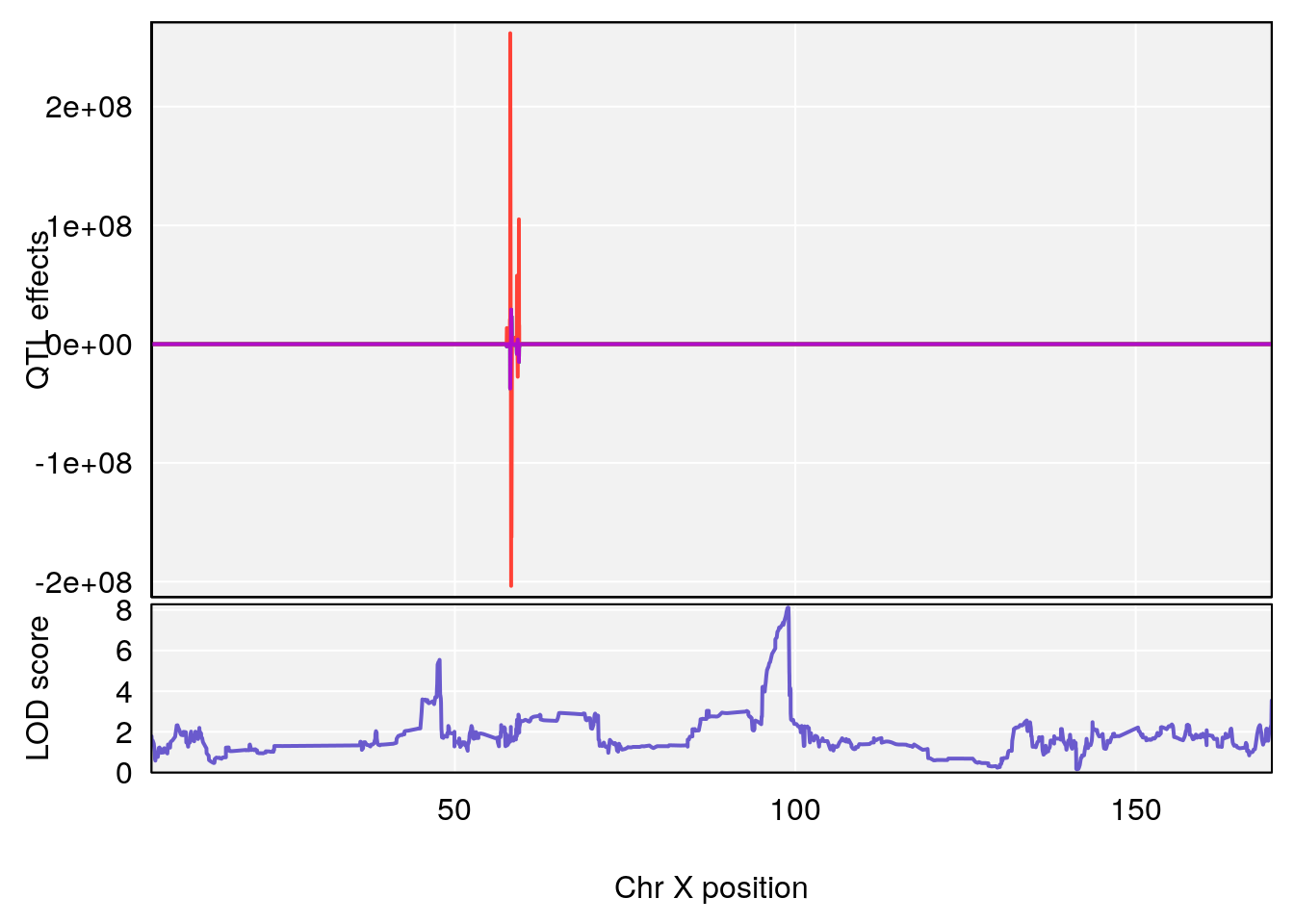
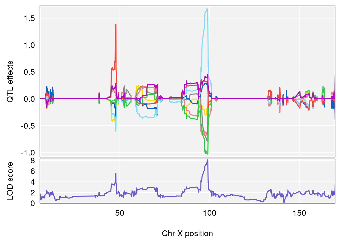
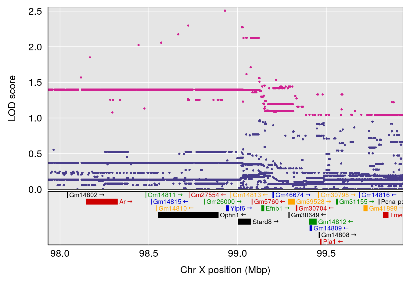
# [1] "EEP_9ms"
# [1] lodindex  lodcolumn chr       pos       lod       ci_lo     ci_hi
# <0 rows> (or 0-length row.names)
# [1] "Tr__sec"
#   lodindex lodcolumn chr      pos     lod    ci_lo    ci_hi
# 1        1    pheno1  19 10.10562 6.24409 10.05116 14.23395
# [1] 1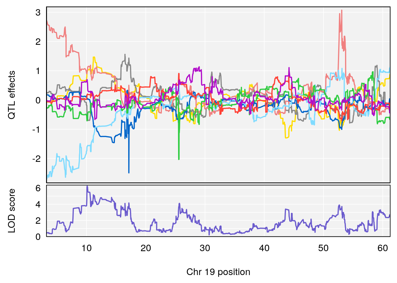
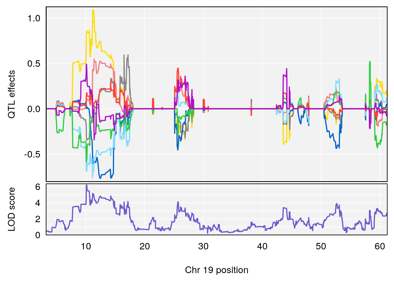
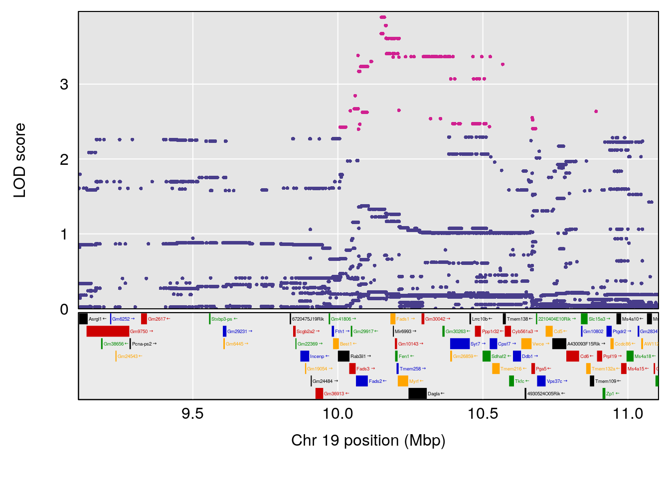
# [1] "TB"
#   lodindex lodcolumn chr      pos      lod    ci_lo    ci_hi
# 1        1    pheno1   X 47.58251 6.793519 45.11958 47.83709
# [1] 1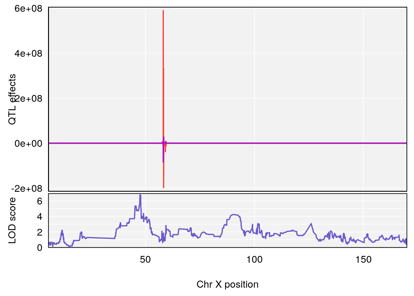
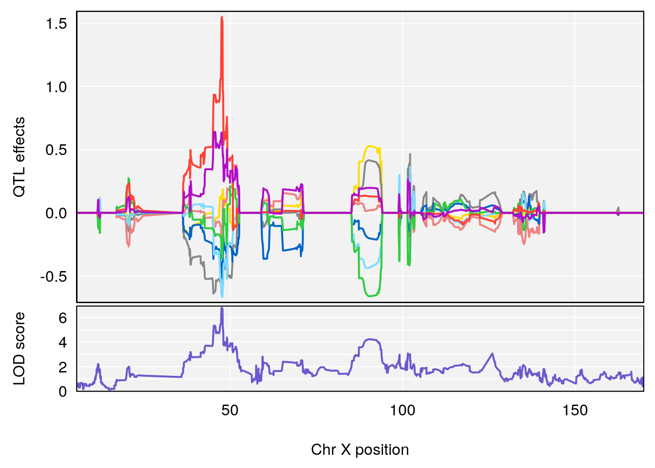
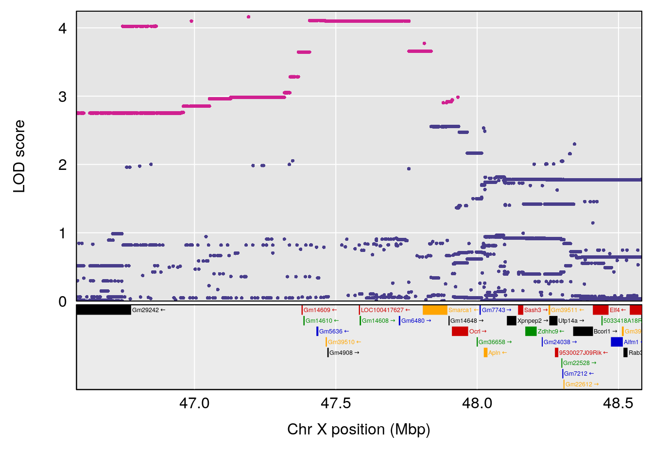
# [1] "TP"
#   lodindex lodcolumn chr       pos      lod     ci_lo     ci_hi
# 1        1    pheno1   5 117.50330 6.917924 117.09802 117.74753
# 2        1    pheno1   9 105.28053 6.371997 104.93950 106.48306
# 3        1    pheno1  14 113.56159 6.136669 108.15378 114.99494
# 4        1    pheno1  17  89.40313 6.230308  51.44475  90.16057
# [1] 1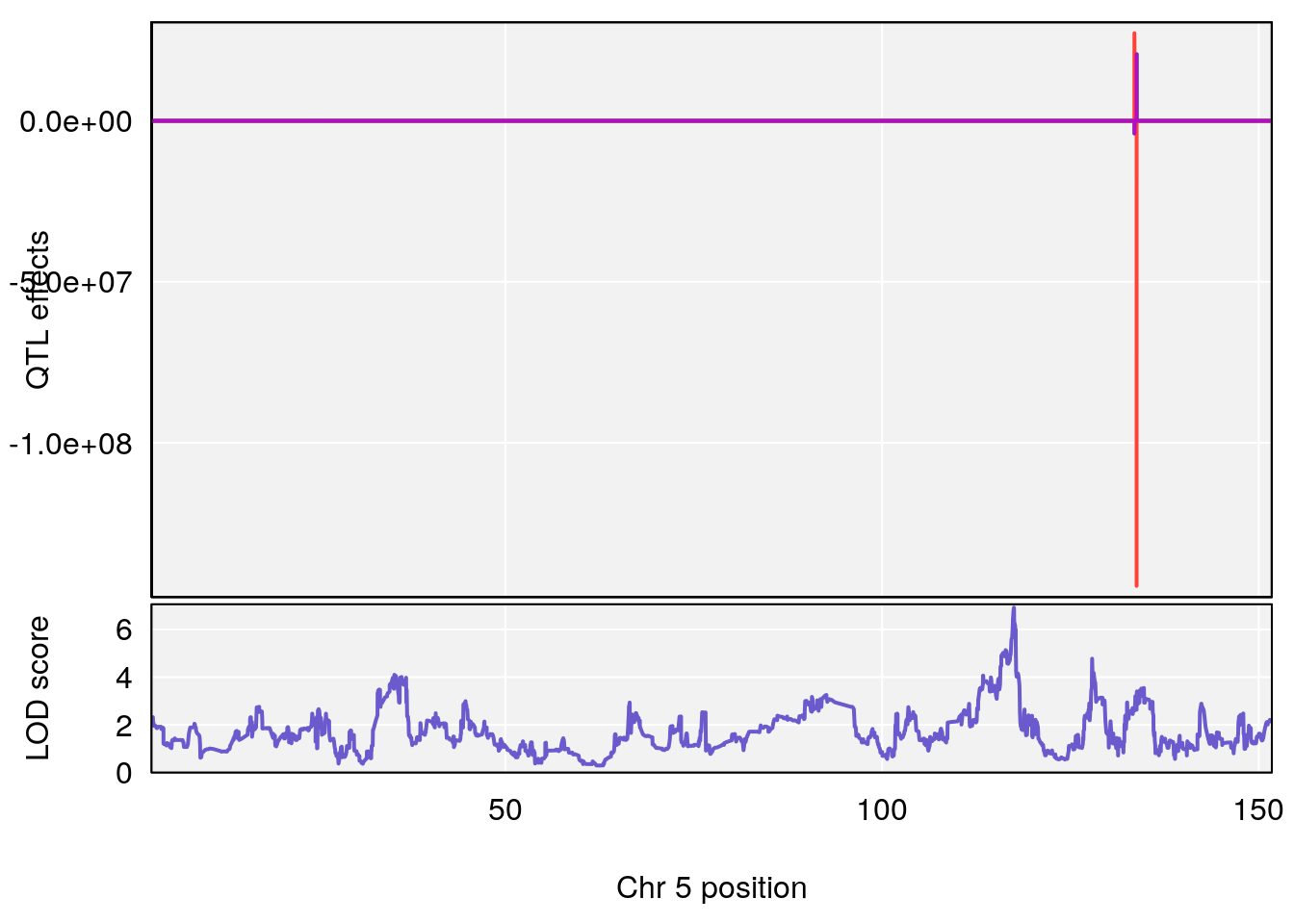
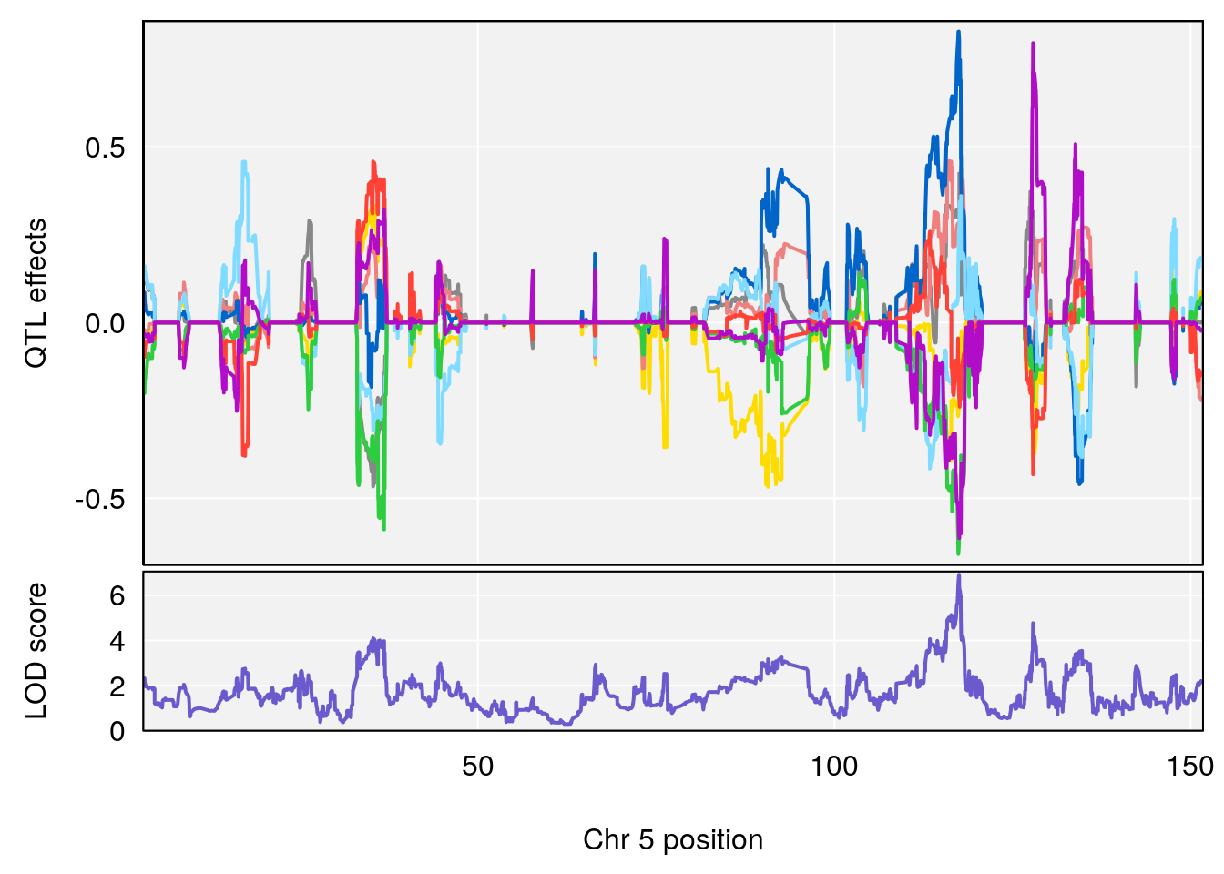
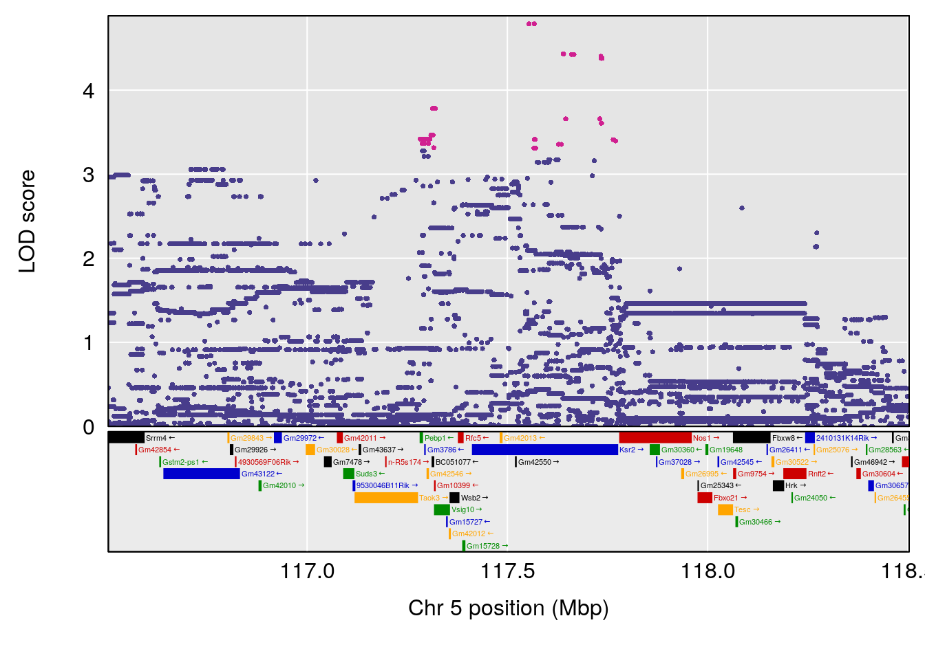
# [1] 2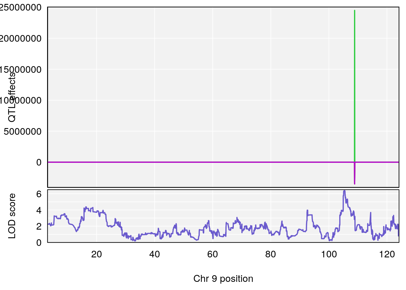
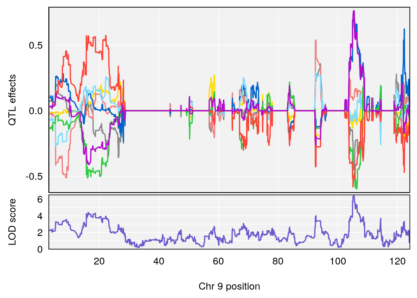
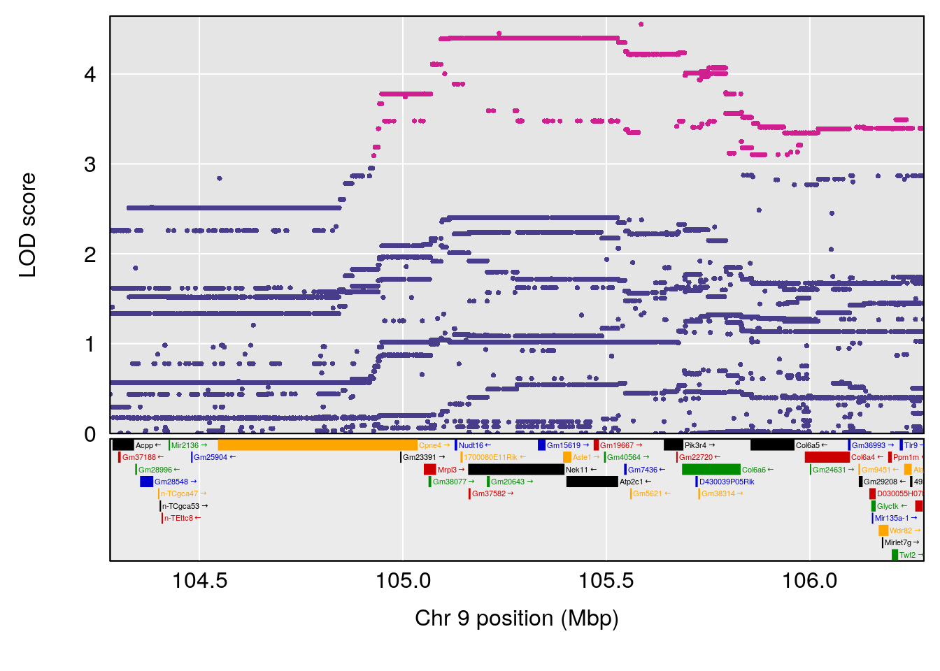
# [1] 3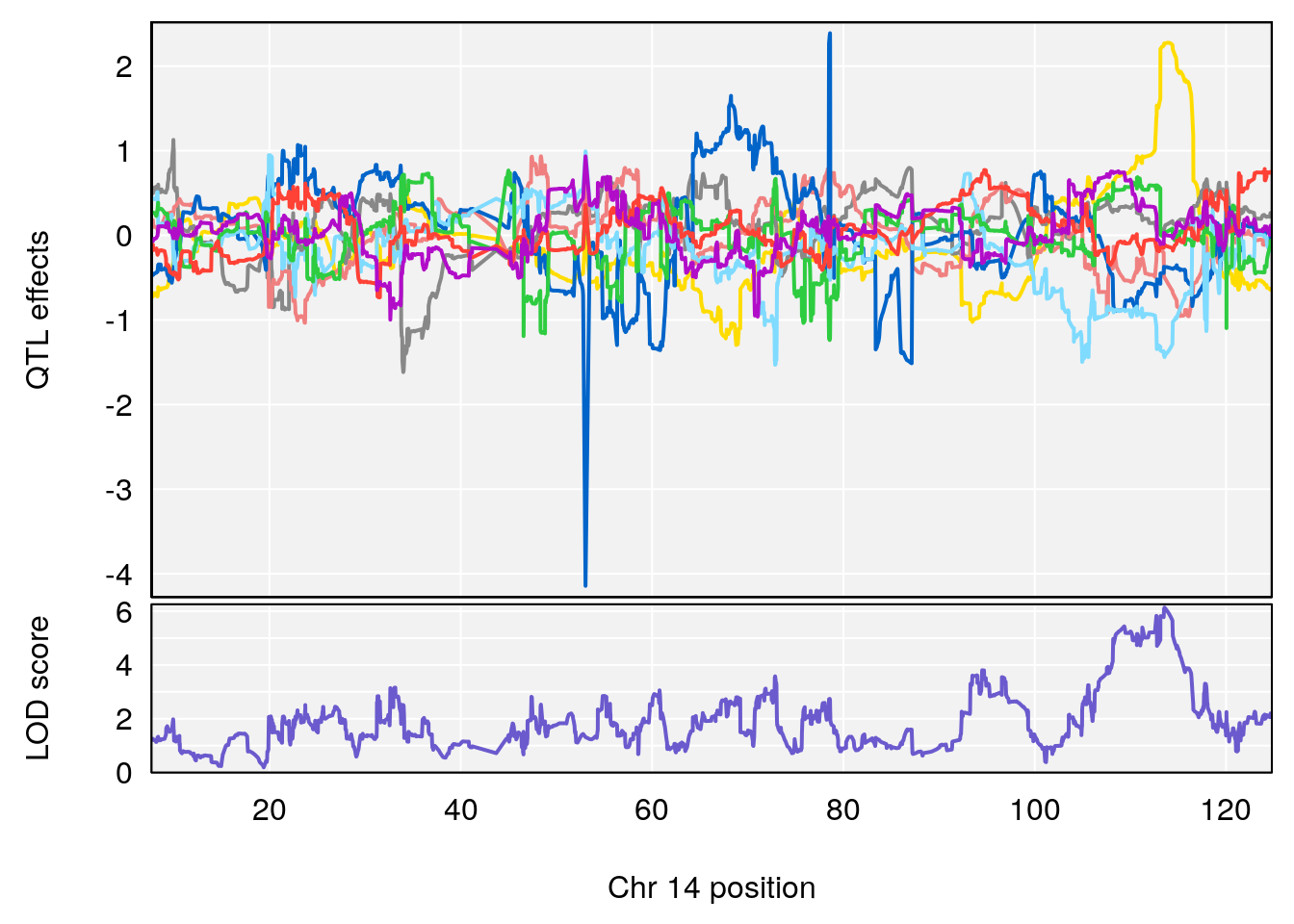
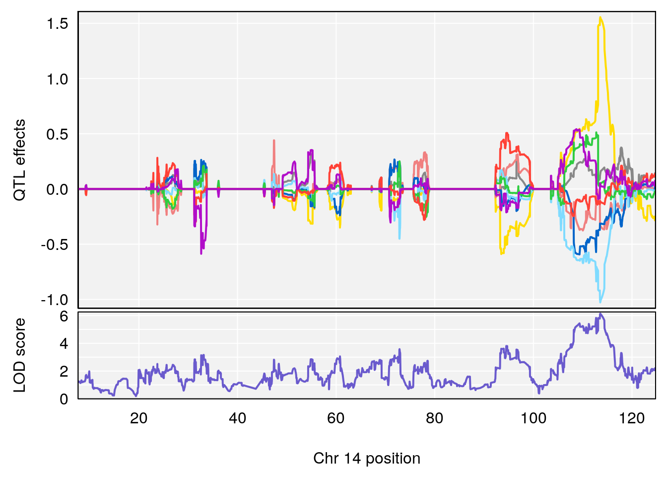
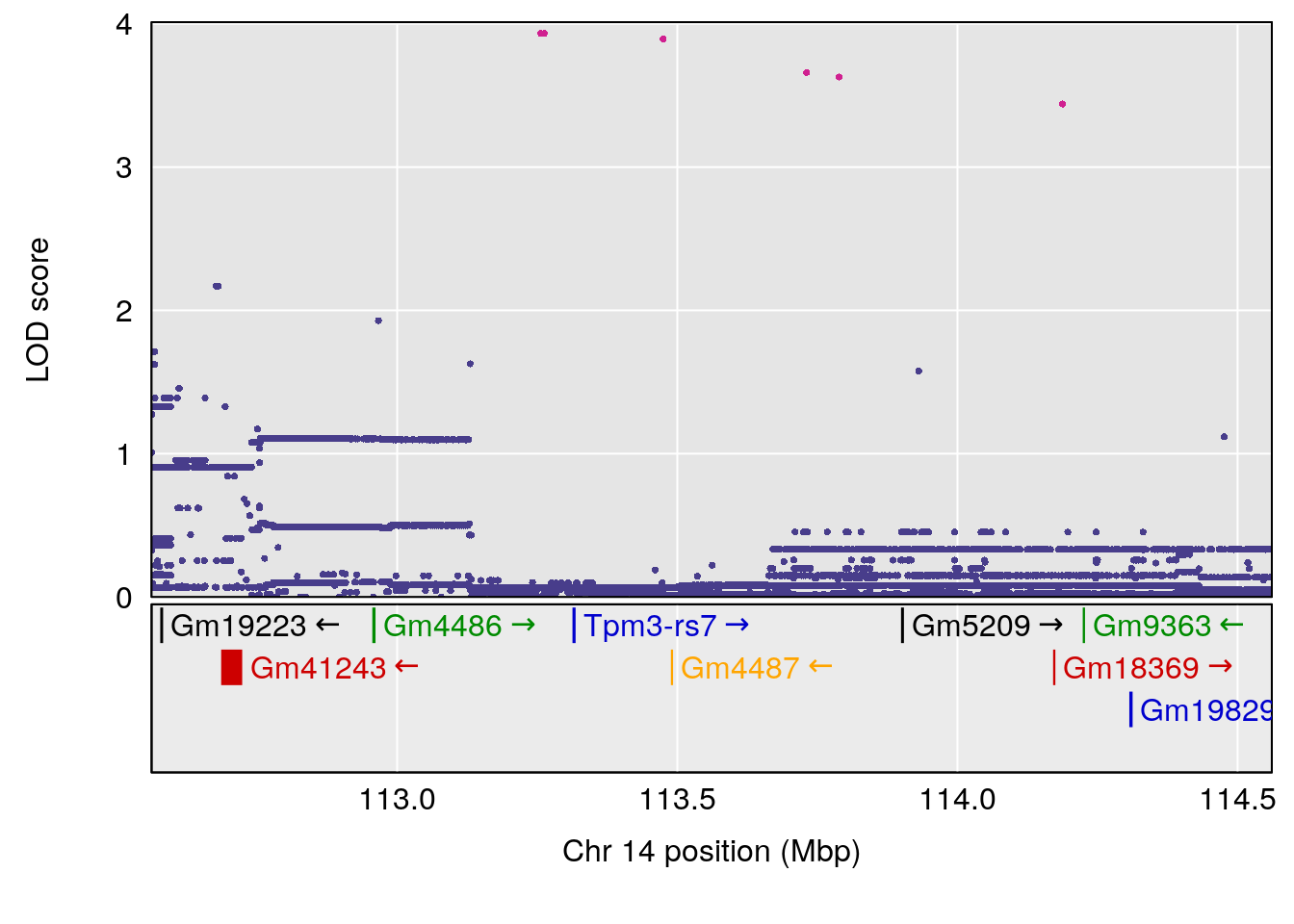
# [1] 4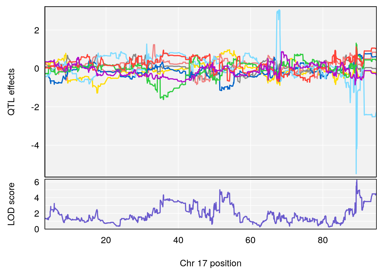
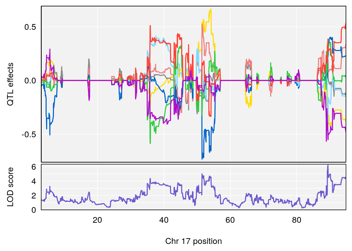
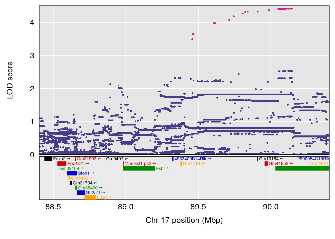
# [1] "Rinx"
#   lodindex lodcolumn chr       pos      lod     ci_lo     ci_hi
# 1        1    pheno1  12 112.54685 6.917175 110.17747 112.60243
# 2        1    pheno1   X  47.48414 9.867438  47.36754  47.83709
# [1] 1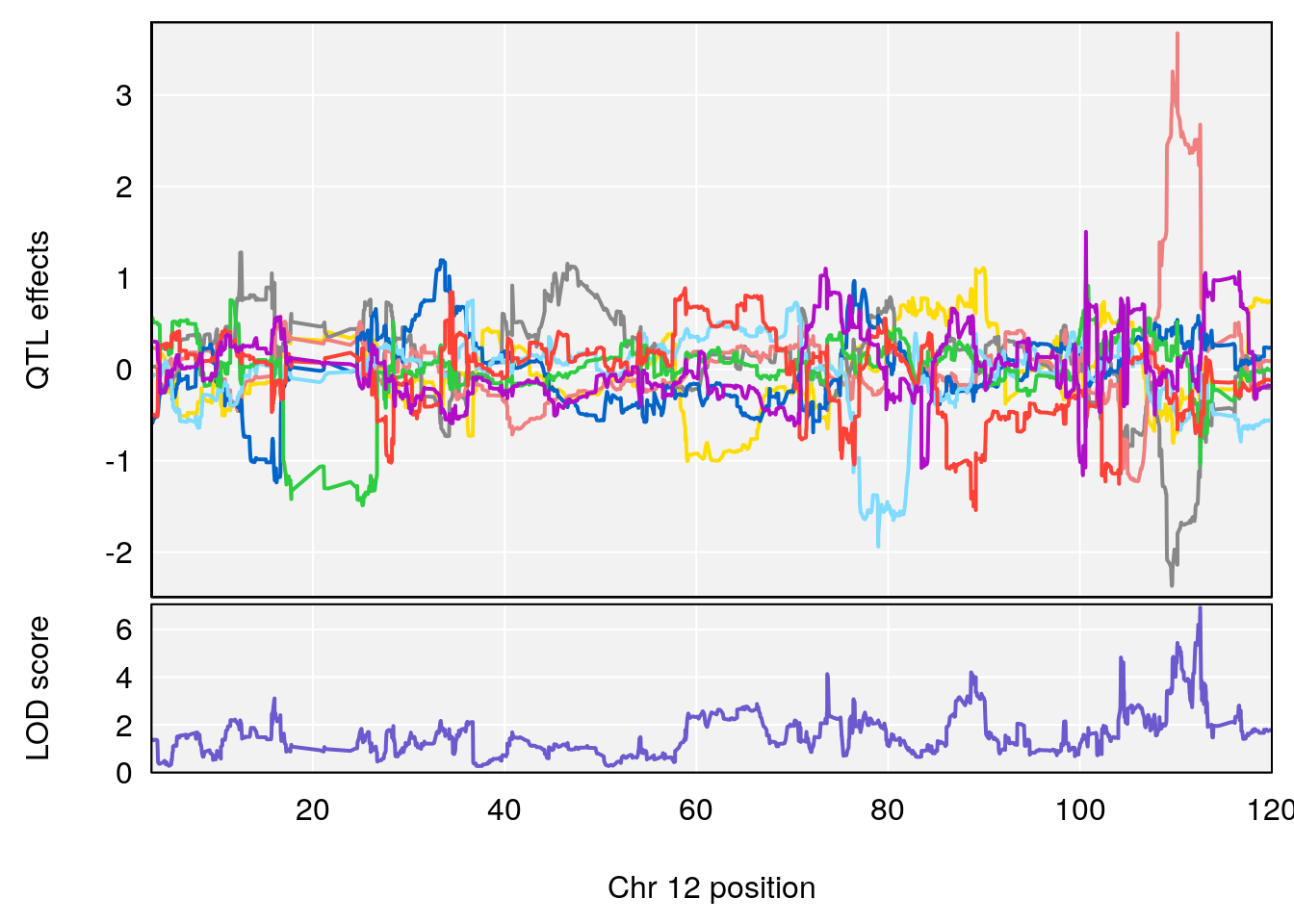
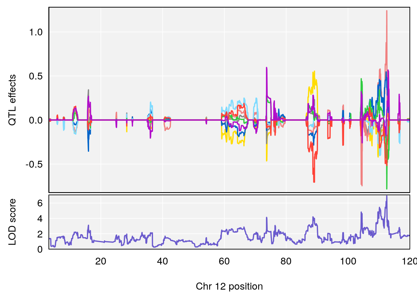
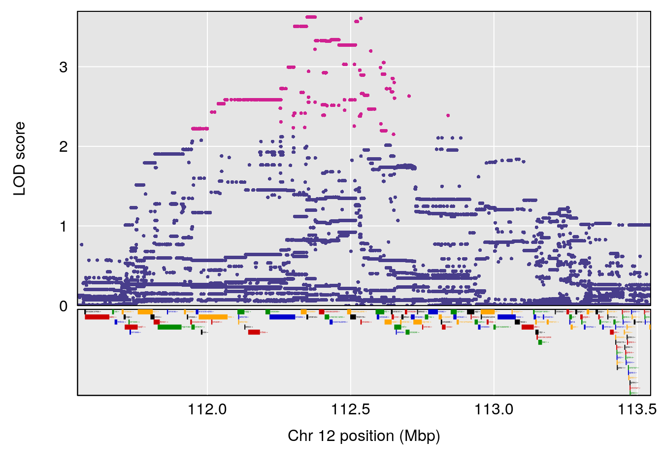
# [1] 2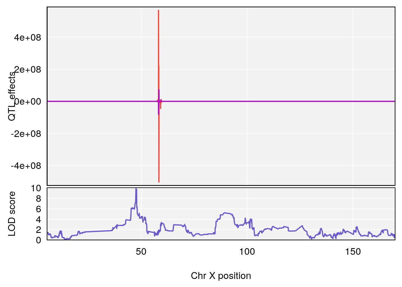
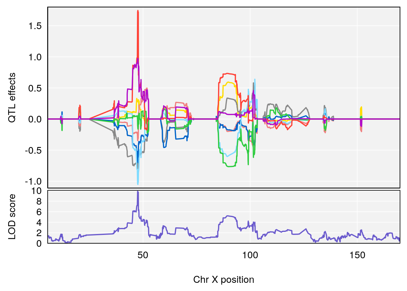
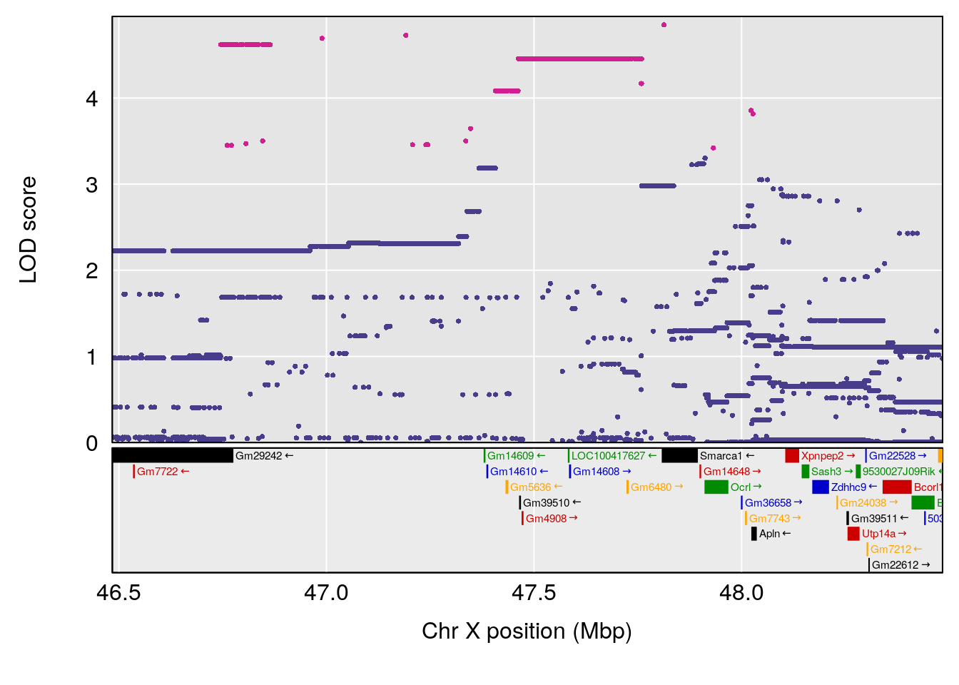
# [1] "Ttot"
#   lodindex lodcolumn chr       pos      lod     ci_lo     ci_hi
# 1        1    pheno1   3 123.59376 6.036933 101.76861 125.85588
# 2        1    pheno1  12  16.02313 6.204214  15.85922  16.64268
# 3        1    pheno1  19  11.00207 6.789937  10.05116  11.37720
# [1] 1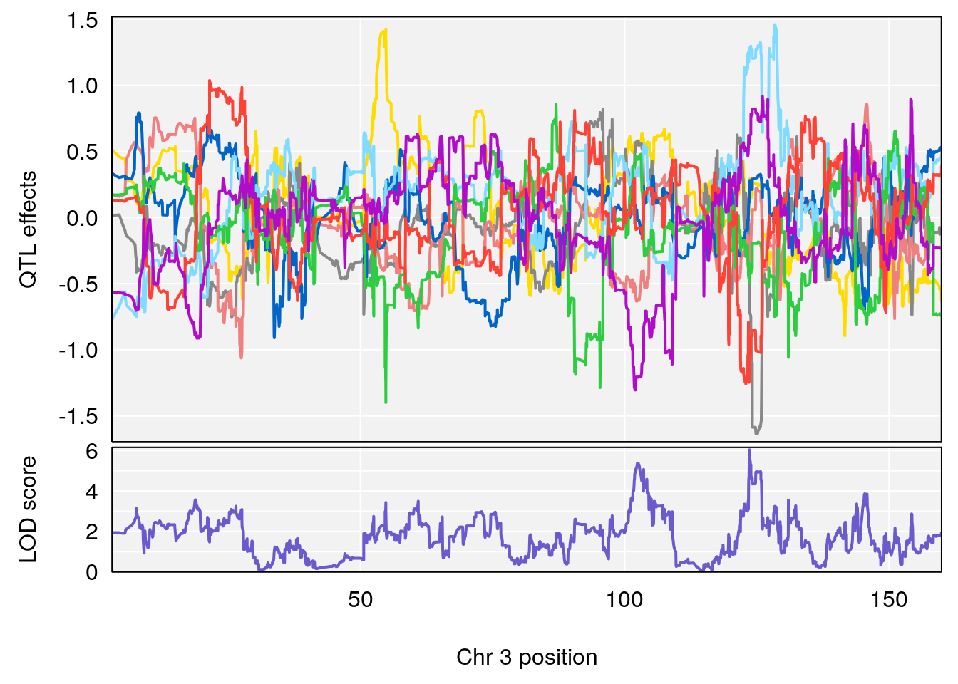
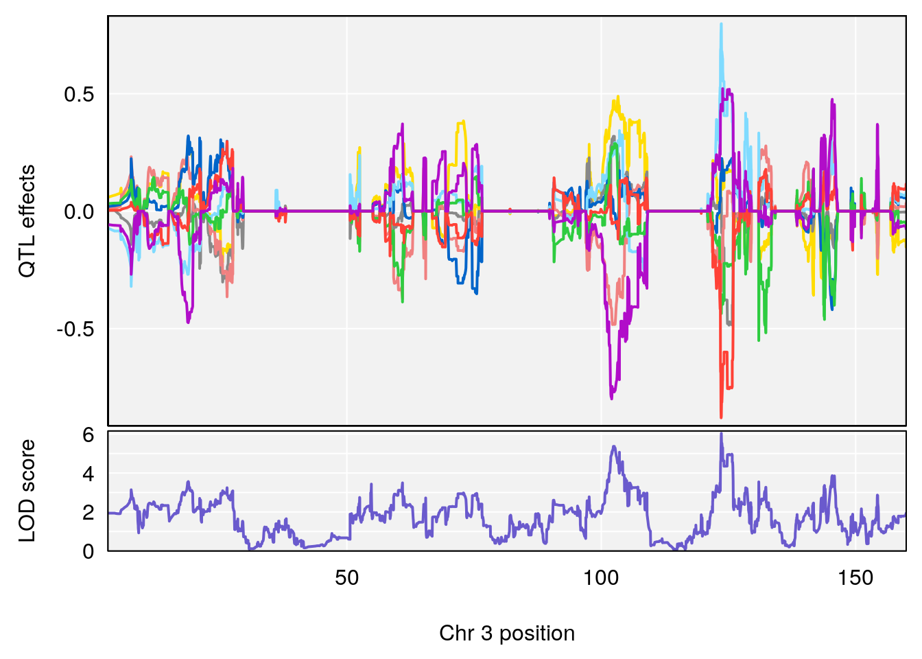
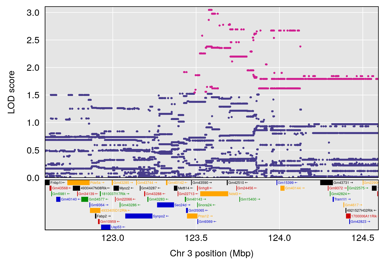
# [1] 2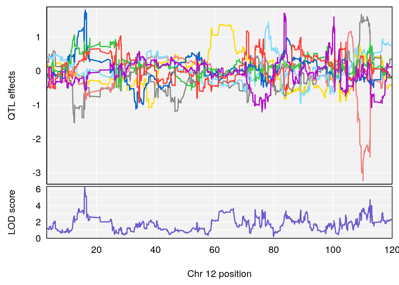
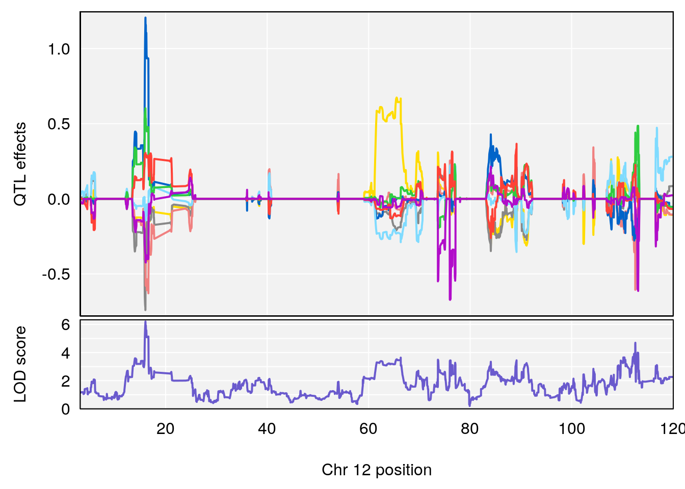
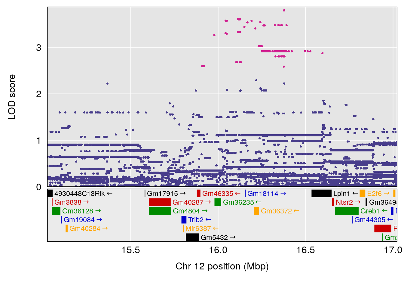
# [1] 3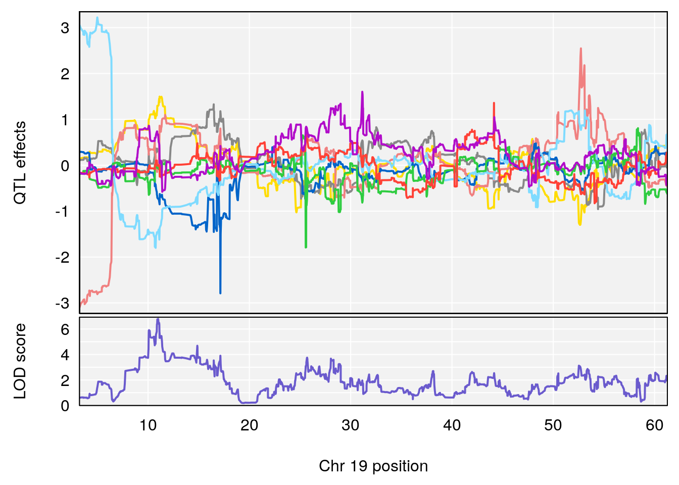
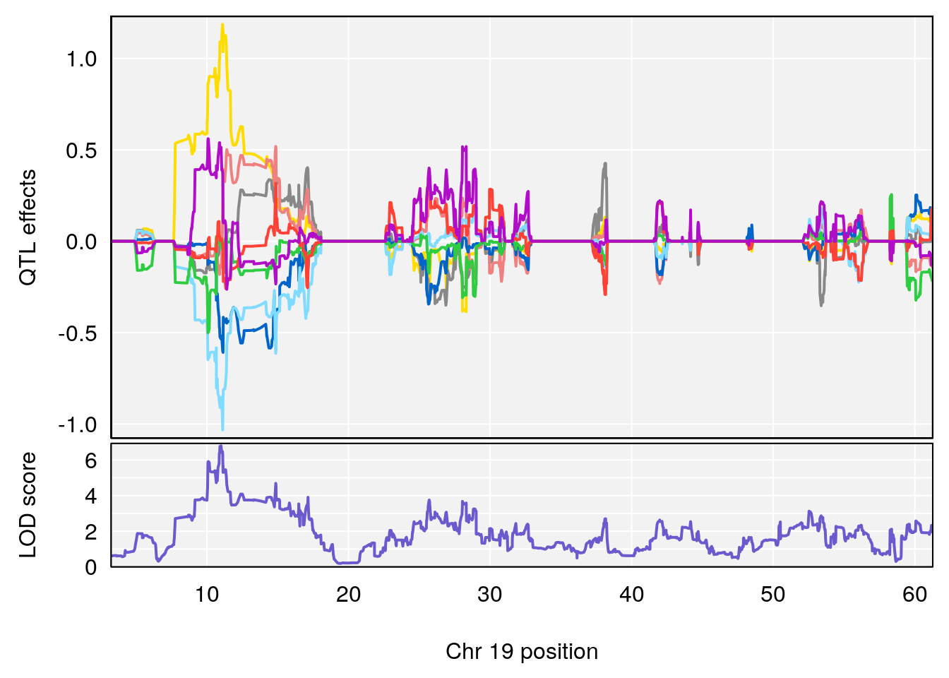
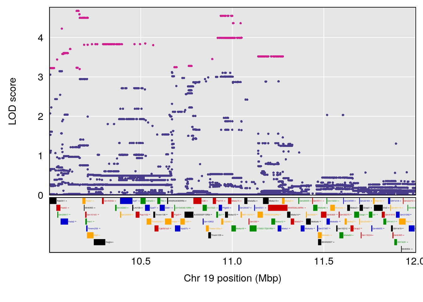
# [1] "duty_cycle"
#   lodindex lodcolumn chr       pos      lod     ci_lo     ci_hi
# 1        1    pheno1   1 31.153698 6.262859 24.098293  62.78409
# 2        1    pheno1   6 80.581747 6.266609 77.729222  85.53938
# 3        1    pheno1   7 61.315114 6.420862 58.532994 131.01270
# 4        1    pheno1  14  9.367214 7.019240  8.041935  10.65151
# [1] 1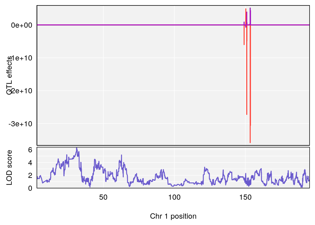
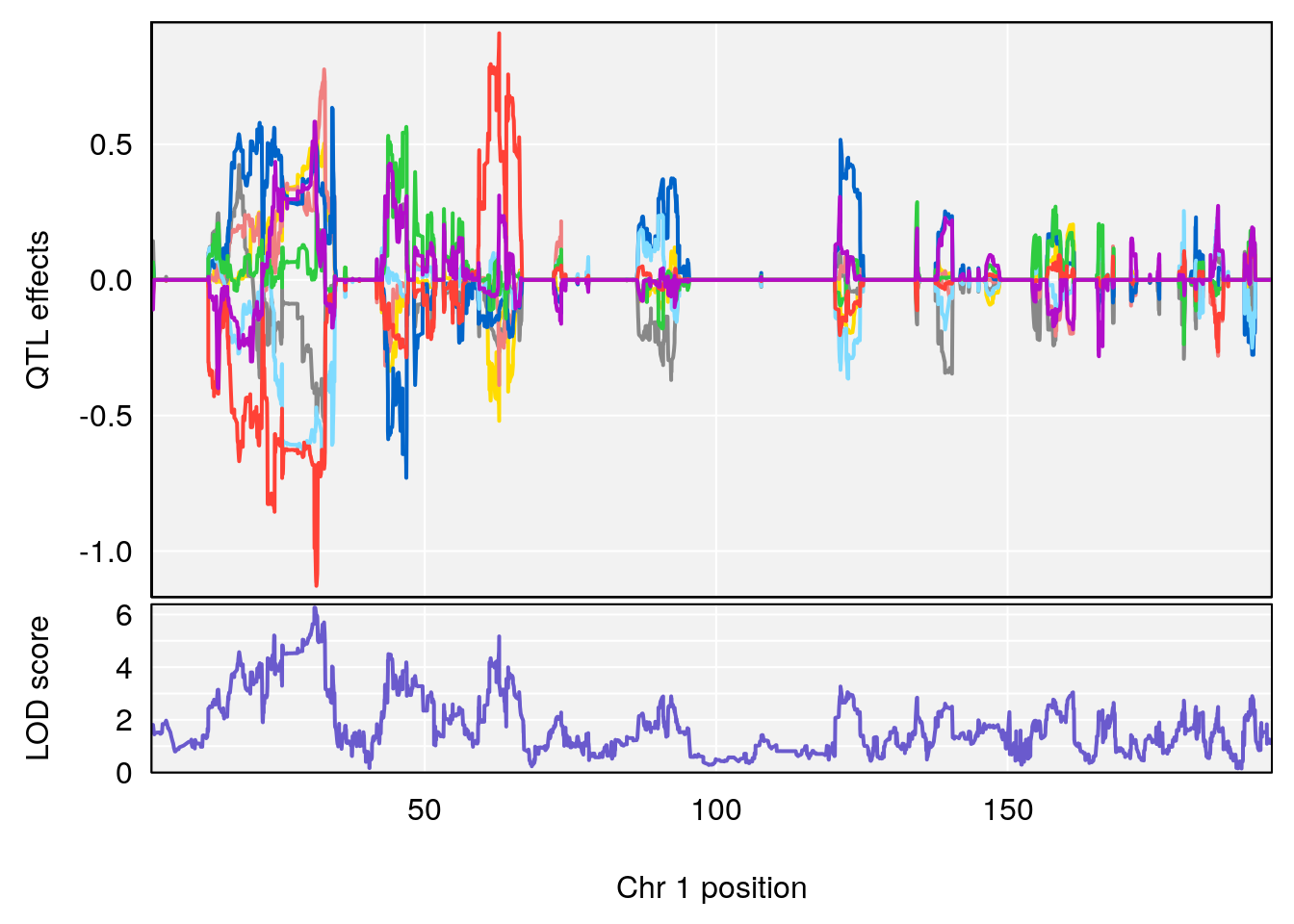
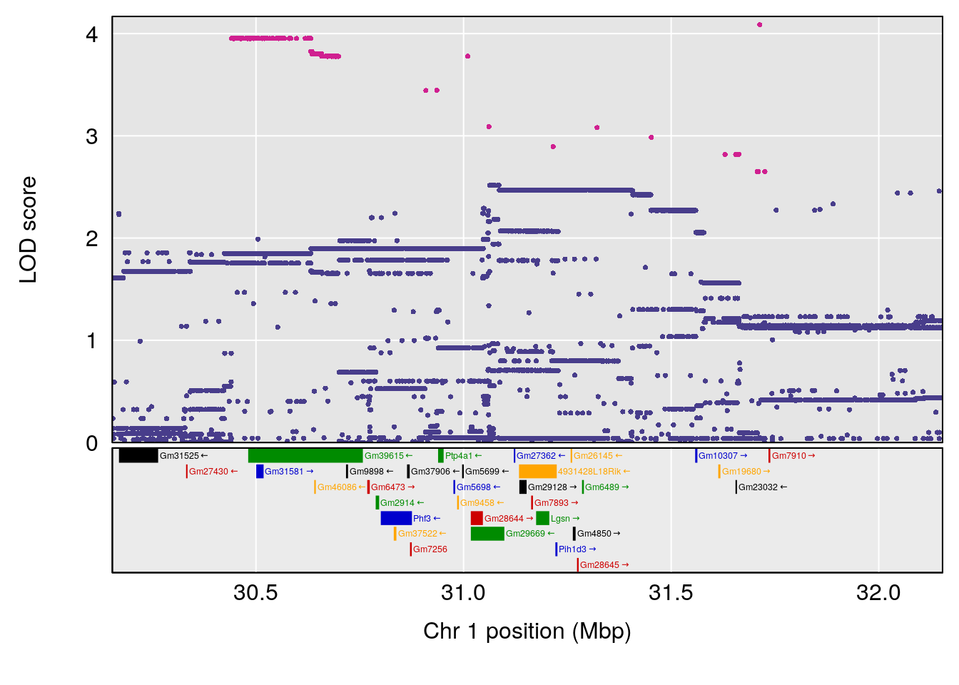
# [1] 2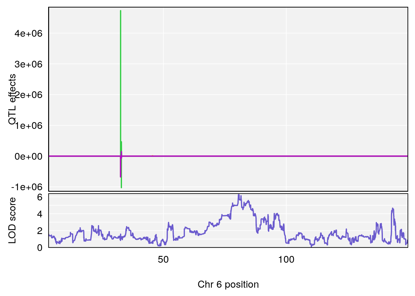
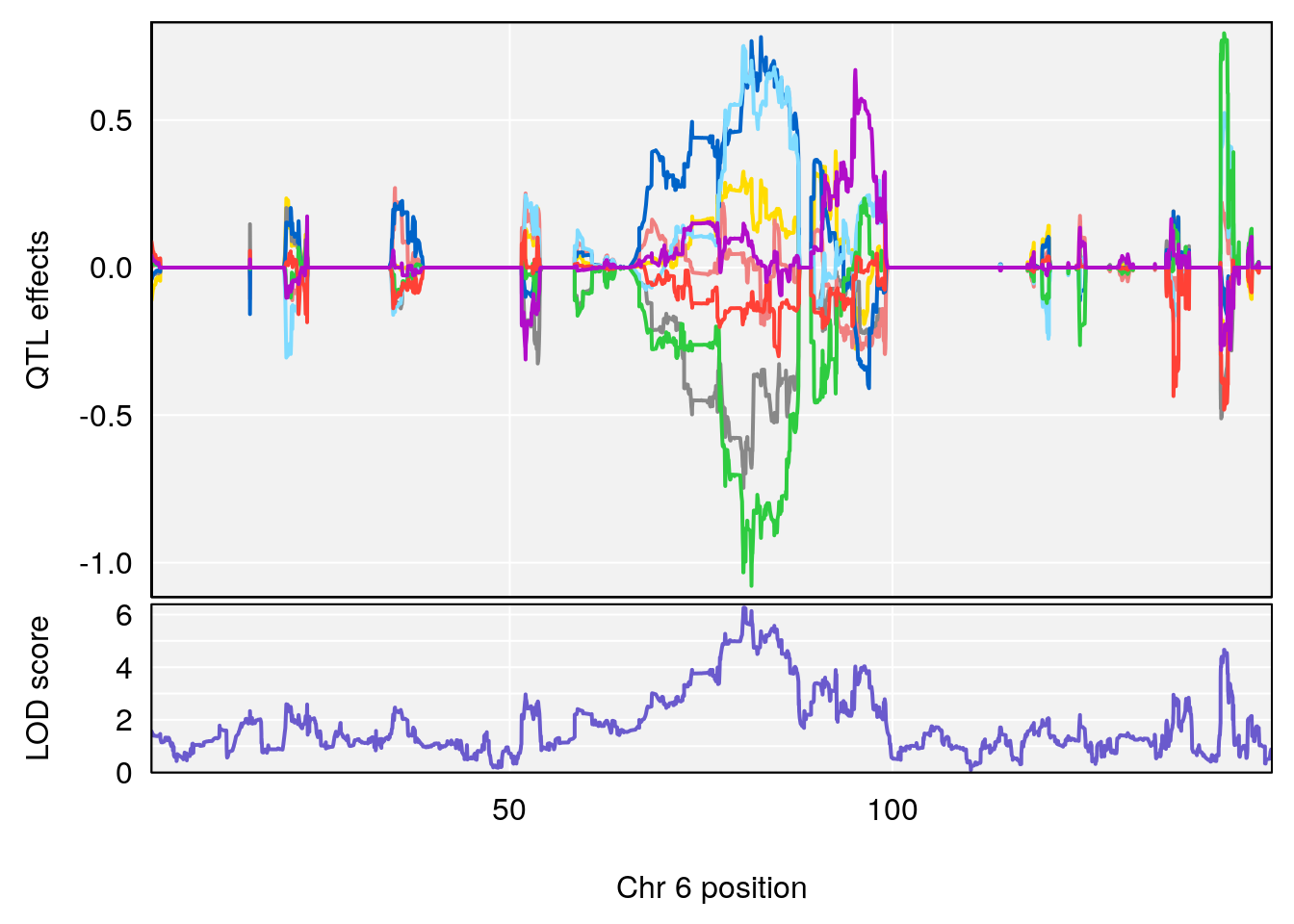
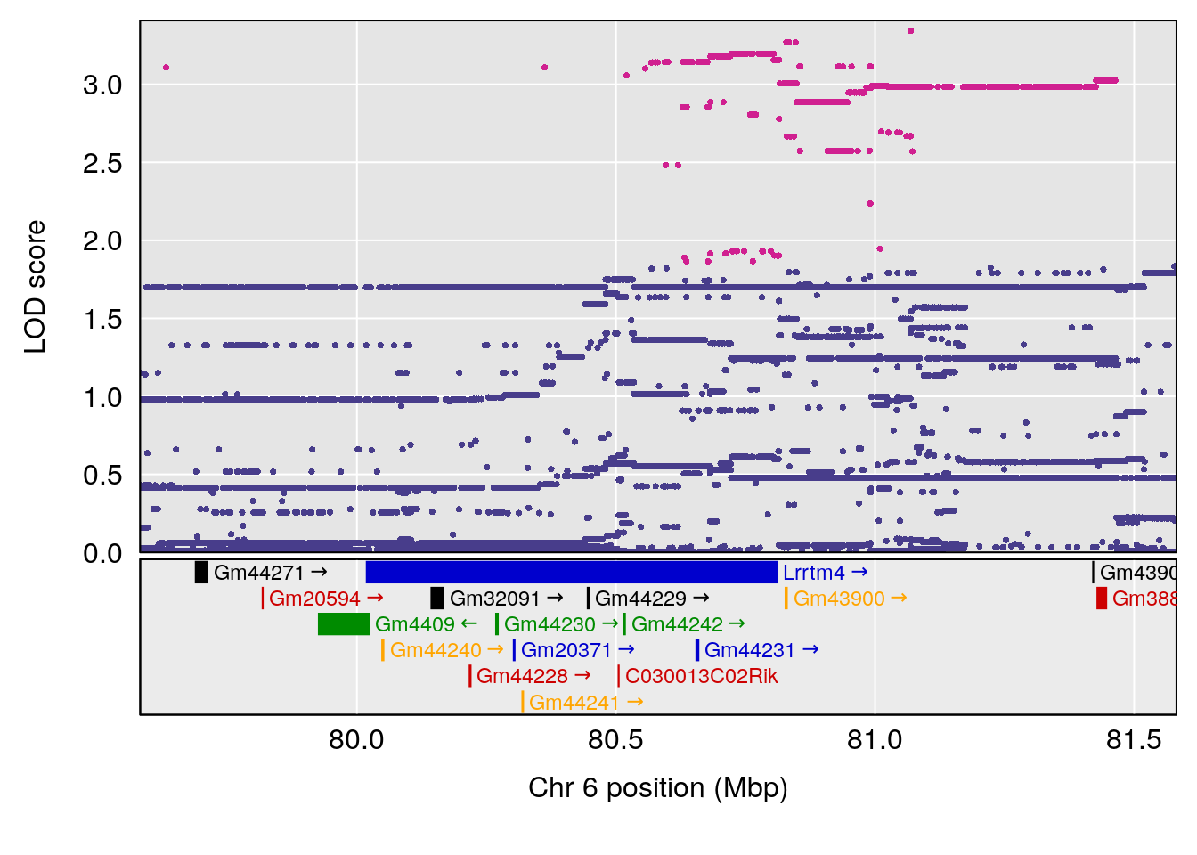
# [1] 3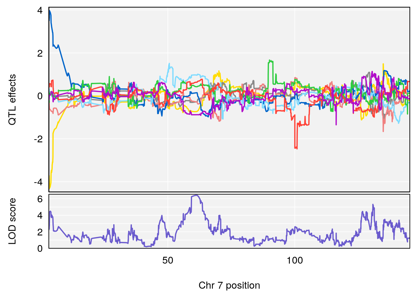
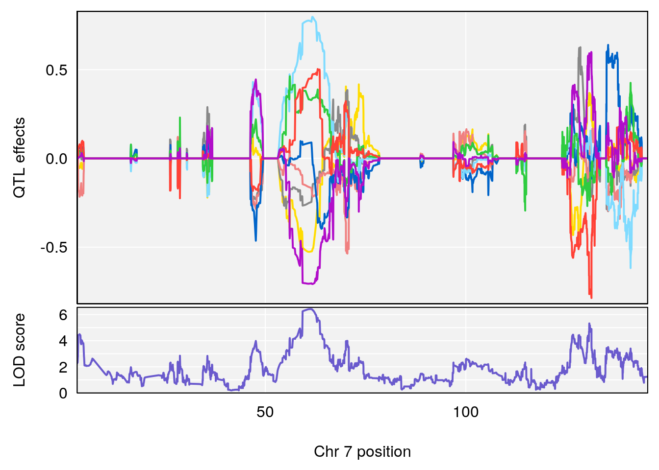
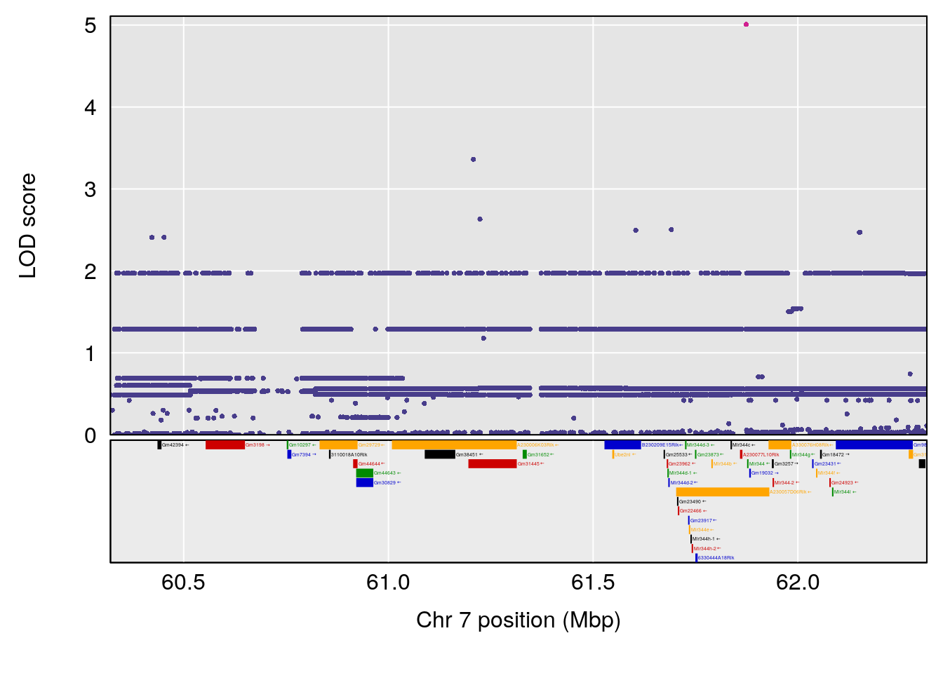
# [1] 4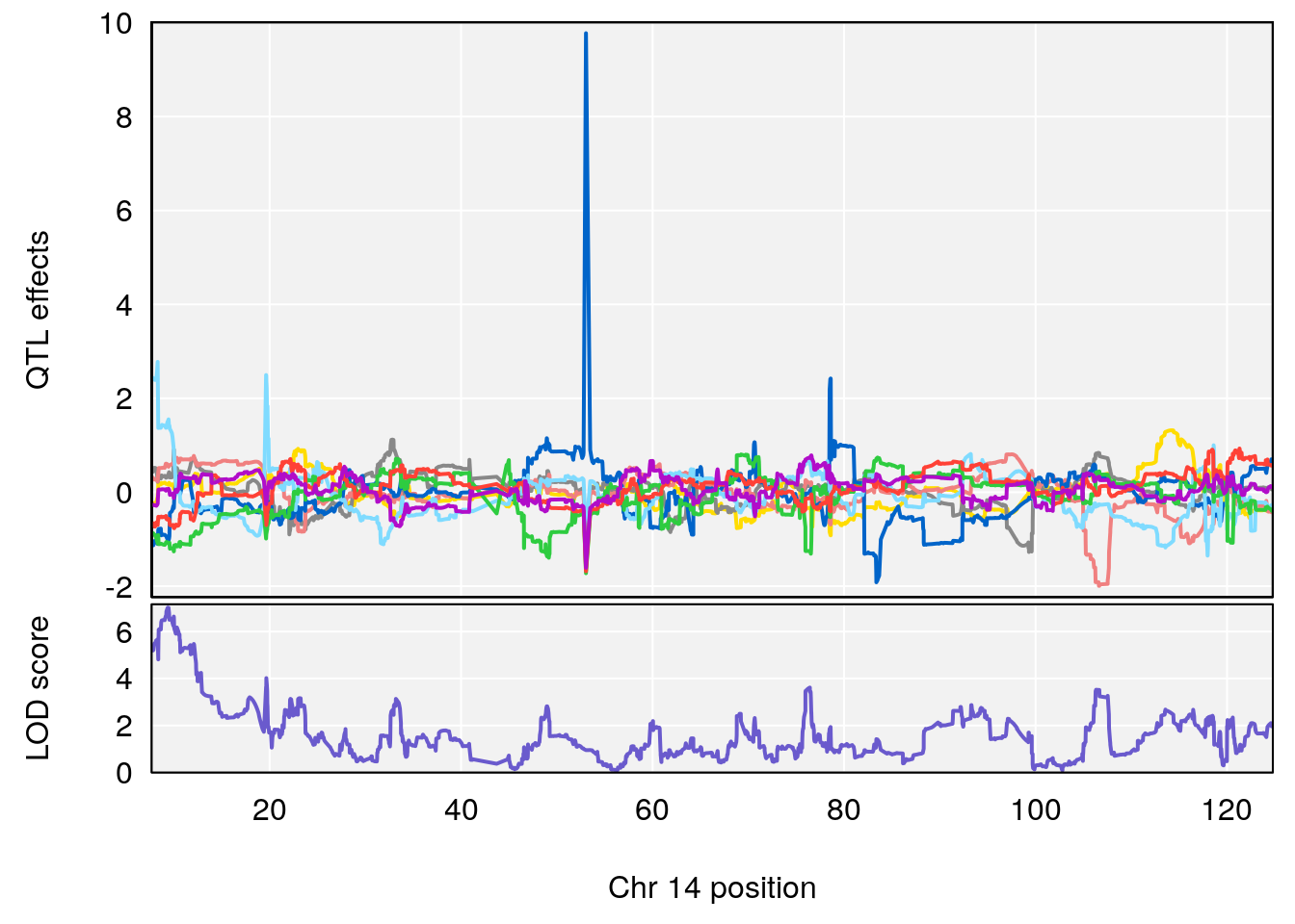
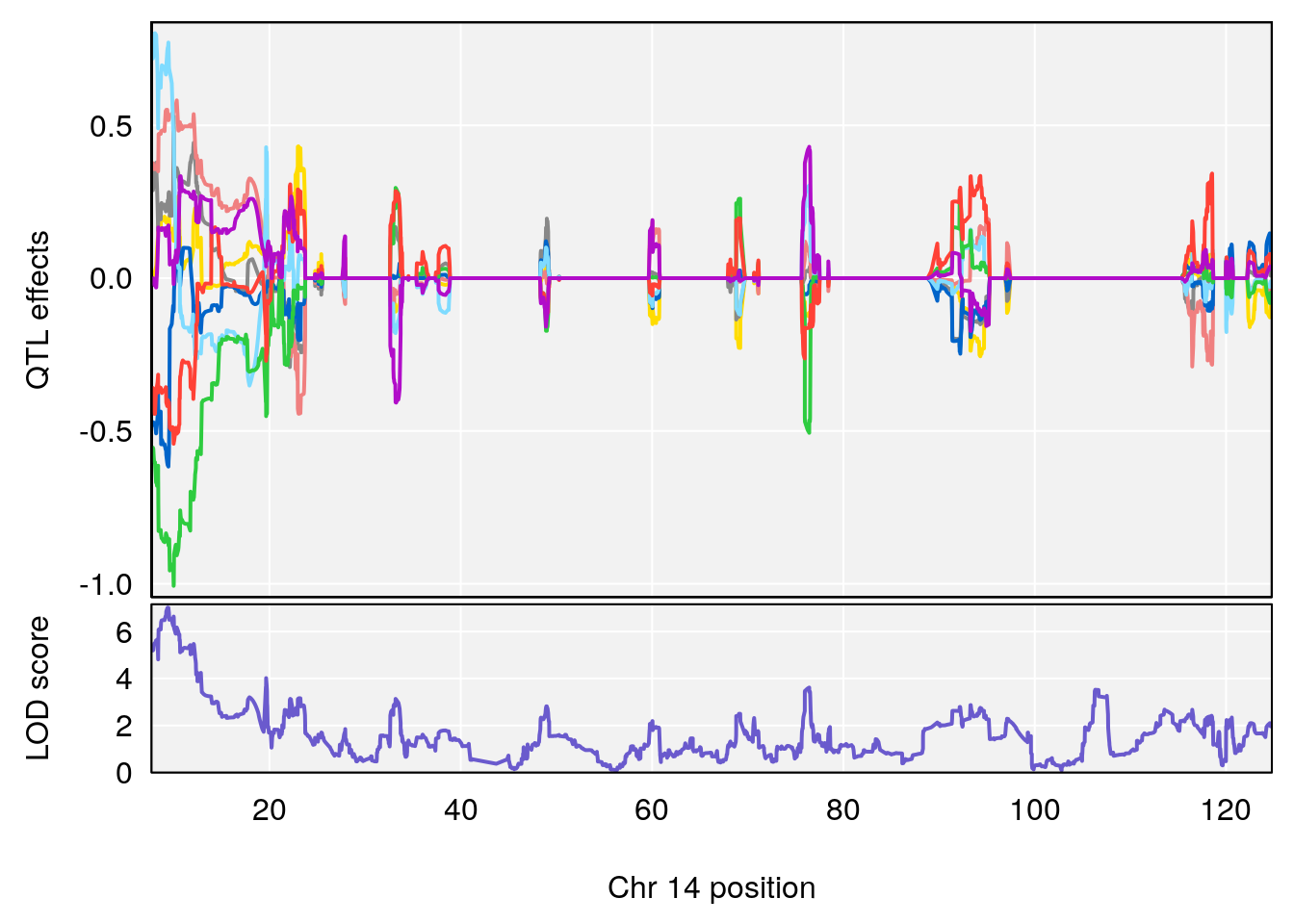
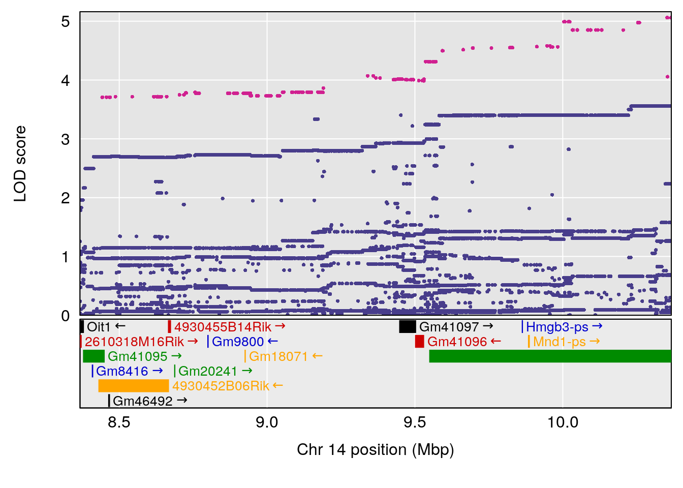
# [1] "resp_flow"
# [1] lodindex  lodcolumn chr       pos       lod       ci_lo     ci_hi
# <0 rows> (or 0-length row.names)
# [1] "insp_flow"
# [1] lodindex  lodcolumn chr       pos       lod       ci_lo     ci_hi
# <0 rows> (or 0-length row.names)
# [1] "exp_flow"
#   lodindex lodcolumn chr     pos      lod    ci_lo    ci_hi
# 1        1    pheno1  14 115.222 6.182287 113.1445 116.3881
# [1] 1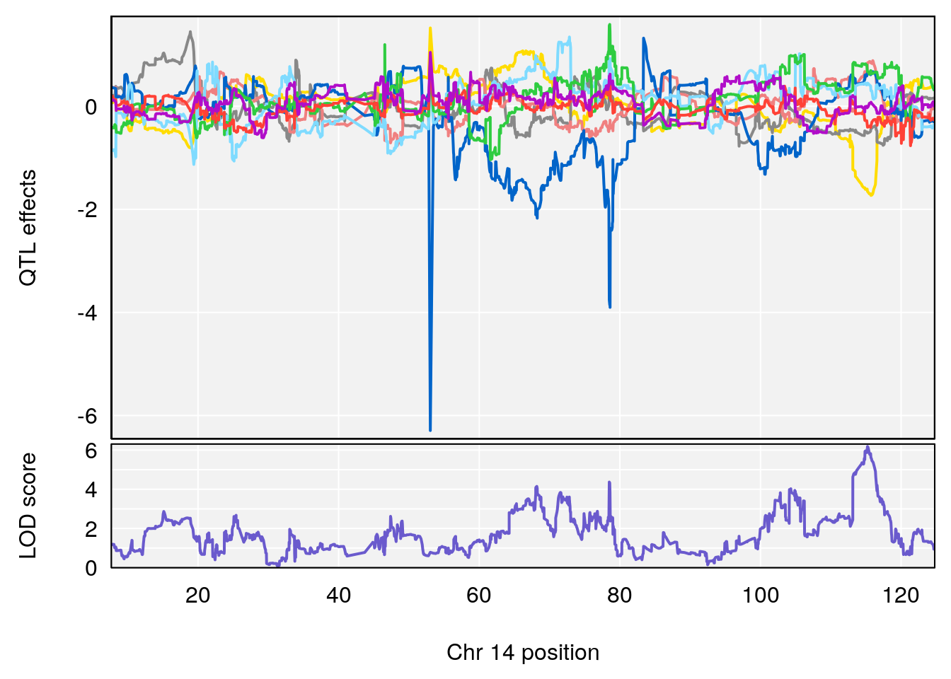
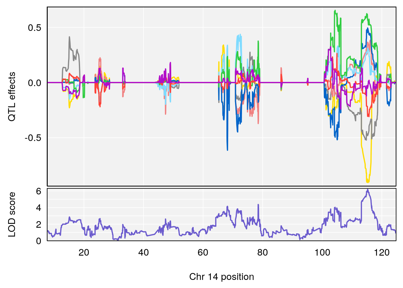
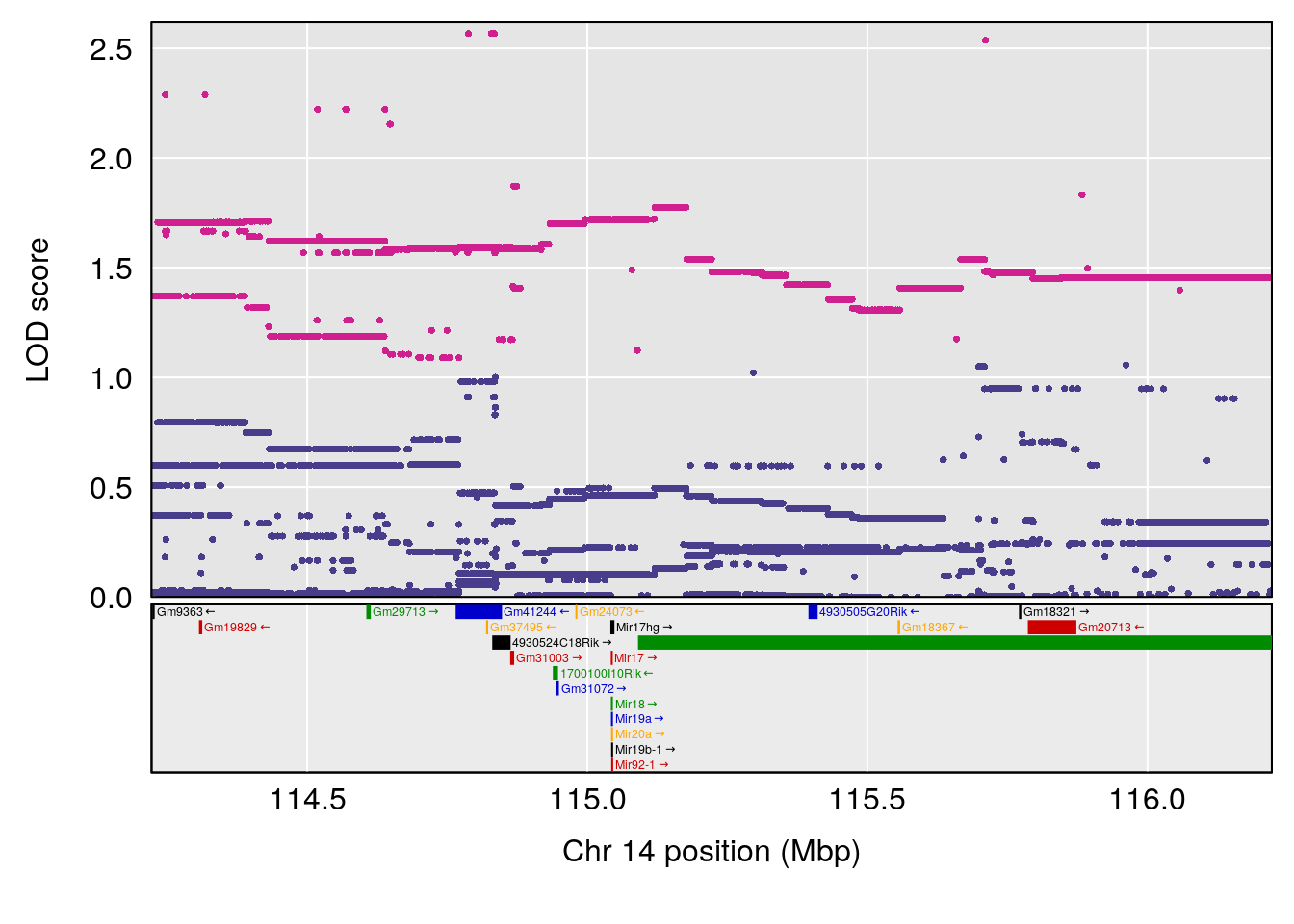
sessionInfo()
# R version 4.0.3 (2020-10-10)
# Platform: x86_64-pc-linux-gnu (64-bit)
# Running under: Ubuntu 20.04.2 LTS
#
# Matrix products: default
# BLAS/LAPACK: /usr/lib/x86_64-linux-gnu/openblas-pthread/libopenblasp-r0.3.8.so
#
# locale:
#  [1] LC_CTYPE=en_US.UTF-8       LC_NUMERIC=C
#  [3] LC_TIME=en_US.UTF-8        LC_COLLATE=en_US.UTF-8
#  [5] LC_MONETARY=en_US.UTF-8    LC_MESSAGES=C
#  [7] LC_PAPER=en_US.UTF-8       LC_NAME=C
#  [9] LC_ADDRESS=C               LC_TELEPHONE=C
# [11] LC_MEASUREMENT=en_US.UTF-8 LC_IDENTIFICATION=C
#
# attached base packages:
# [1] parallel  stats     graphics  grDevices utils     datasets  methods
# [8] base
#
# other attached packages:
#  [1] qtl_1.47-9      patchwork_1.1.1 furrr_0.2.2     future_1.21.0
#  [5] cowplot_1.1.1   forcats_0.5.1   stringr_1.4.0   dplyr_1.0.4
#  [9] purrr_0.3.4     readr_1.4.0     tidyr_1.1.2     tibble_3.0.6
# [13] tidyverse_1.3.0 openxlsx_4.2.3  abind_1.4-5     regress_1.3-21
# [17] survival_3.2-7  qtl2_0.24       GGally_2.1.0    gridExtra_2.3
# [21] ggplot2_3.3.3   workflowr_1.6.2
#
# loaded via a namespace (and not attached):
#  [1] fs_1.5.0           lubridate_1.7.9.2  bit64_4.0.5        RColorBrewer_1.1-2
#  [5] httr_1.4.2         rprojroot_2.0.2    tools_4.0.3        backports_1.2.1
#  [9] R6_2.5.0           DBI_1.1.1          colorspace_2.0-0   withr_2.4.1
# [13] tidyselect_1.1.0   bit_4.0.4          compiler_4.0.3     git2r_0.28.0
# [17] cli_2.3.0          rvest_0.3.6        xml2_1.3.2         labeling_0.4.2
# [21] scales_1.1.1       digest_0.6.27      rmarkdown_2.6      pkgconfig_2.0.3
# [25] htmltools_0.5.1.1  parallelly_1.23.0  highr_0.8          dbplyr_2.1.0
# [29] fastmap_1.1.0      rlang_1.0.2        readxl_1.3.1       rstudioapi_0.13
# [33] RSQLite_2.2.3      farver_2.0.3       generics_0.1.0     jsonlite_1.7.2
# [37] zip_2.1.1          magrittr_2.0.1     Matrix_1.3-2       Rcpp_1.0.6
# [41] munsell_0.5.0      lifecycle_1.0.0    stringi_1.5.3      whisker_0.4
# [45] yaml_2.2.1         plyr_1.8.6         grid_4.0.3         blob_1.2.1
# [49] listenv_0.8.0      promises_1.2.0.1   crayon_1.4.1       lattice_0.20-41
# [53] haven_2.3.1        splines_4.0.3      hms_1.0.0          knitr_1.31
# [57] pillar_1.4.7       codetools_0.2-18   reprex_1.0.0       glue_1.4.2
# [61] evaluate_0.14      data.table_1.13.6  modelr_0.1.8       vctrs_0.3.6
# [65] httpuv_1.5.5       cellranger_1.1.0   gtable_0.3.0       reshape_0.8.8
# [69] assertthat_0.2.1   cachem_1.0.4       xfun_0.21          broom_0.7.4
# [73] later_1.1.0.1      memoise_2.0.0      globals_0.14.0     ellipsis_0.3.1
This R Markdown site was created with workflowr