Spatial omics
Recipes for spatial-omics datasets: cells or spots measured in a tissue section. The panel and charts are described in Spatial omics and Distribution charts.
Open a dataset in the spatial view
- Open the dataset (in the demo: the spatial-omics folder of the gallery).
- If it has a tissue image, the image opens first: pick Spatial omics in the plot-type dropdown. If its cells have z coordinates you can pick Spatial omics 3D instead.
- Click
 Spatial omics controls to open the panel.
A dataset with no image and no volume (such as seqFISH) opens directly in a spatial view. A dataset with a reference volume (such as the Allen Brain Cell Atlas) opens the volume in the Image view first.
Colour observations by cell type or cluster
- In the panel, Observations → Colour by, choose Group.
- Pick the column in the Groups dropdown. Related columns (for example k-means with k = 2 … 10) are listed once, with a second dropdown for the variant.
Hide some groups
Untick their checkboxes in the Groups list. All groups (total) shows or hides them all.
Change a group's colour
Click the group's colour dot, pick a colour, or click Reset to default. Custom colours reset when you open another dataset.
Colour observations by a gene
- Colour by → Gene.
- Type part of the gene name in Search N genes… and pick it.
- Adjust the scale: Colormap (empty means "match the image"), Log scale, and Clip outliers (None, 1%, 2% or 5%).
Colour by a measurement
Colour by → Measurement, then pick a column such as total counts. Options show their unit.
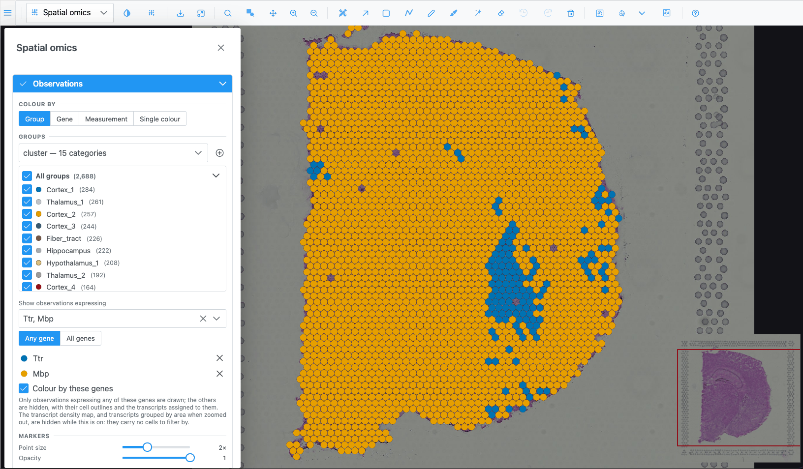
Show only cells that express given genes
- In Show observations expressing, pick one or more genes.
- With several genes, choose Any gene or All genes.
- Leave Colour by these genes on to colour each cell by the picked gene it expresses most; turn it off to keep the Colour by colours.
Cells that do not express the genes (value 0) are hidden, with their outlines and transcripts. Click a gene's swatch to change its colour and the icon used on 2D markers; click × to remove it.
Make markers bigger or more transparent
Under Markers, set Point size (0.25× to 5×) and Opacity (0.1 to 1). These only change how markers are drawn, not what is selected.
Show cell outlines instead of dots
When the dataset has cell segmentations:
- Set Show as to Cell segmentations.
- In 2D, choose View cells as: Fill, Outline or Both, and which Boundaries to draw (for example cell and nucleus).
- Set the fill opacity.
In 3D, choose By cell type (one surface per type) or Individual cells.
Select observations inside a region
- Draw one or more regions on the spatial view with any region tool (F, R, the wand…).
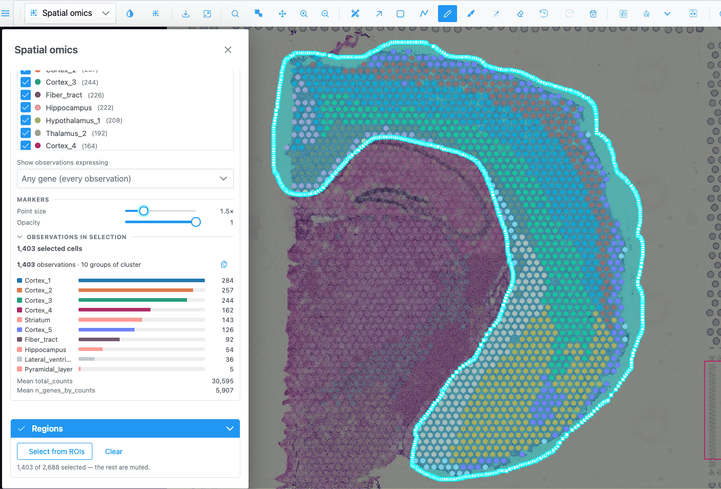
- In the panel, expand Regions and click Select from ROIs.
- Click Clear to drop the selection.
The selected observations stay bright and the rest are muted. The charts, the Observations in selection summary and the embedding follow the selection. Regions can stay hidden while you select (the Regions switch is off by default).
Select cells inside a 3D brain region (atlas)
For a dataset with a reference volume and no tissue image (such as the Allen Brain Cell Atlas):
- Pick Spatial omics 3D.
- Open the Region Editor and pick one or more classes in its class tree (click; Shift-click to add). You can also click a region's surface in the 3D view with Selection mode.
- In the Spatial omics panel, Regions → Select from ROIs. The hint says it selects inside the volume of the picked classes.
Without picked classes, a region drawn over the 3D cloud cuts through its full depth as seen from the camera. Orbit and draw again to cut from another angle.
Select a whole group by clicking
- Click a group's name in the Groups list. Click again to clear.
- Click a marker on the map to select its group. Click again to clear. (Not while colouring by a gene.)
Count what is in the selection
Look at Observations in selection: number of observations, number of groups and a bar per group. copies the counts as tab-separated text, ready to paste into a spreadsheet.
Compare a gene across clusters
- Colour by → Gene and pick the gene.
- Expand Distribution, choose Violin or Box, and set the grouping to the cluster column.
With a selection, only the selected observations are charted.
Build a heatmap of marker genes
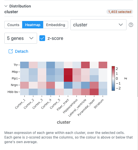
- Expand Distribution and choose Heatmap.
- Pick the grouping column (the heatmap's columns).
- Pick the genes in Pick genes for the rows.
- Keep z-score on to compare genes on their own scale; turn it off to compare raw means.
If the data source supports it, All genes shows every gene against every cell, zoomable: scroll to zoom (Shift: genes only, Alt: cells only), drag to pan, double-click to reset, click a gene to colour the map by it.
Select cells by lassoing an embedding
- Colour by → Group so the embedding is coloured like the map.
- Distribution → Embedding. If there are several (UMAP, PCA, t-SNE), choose one.
- Use the lasso or box tool in the chart's toolbar and draw around points.
Those cells are selected on the map too. An empty lasso clears the selection.
Compute a t-SNE in the browser
Offered when the dataset has a PCA, no t-SNE, and at most 5,000 observations:
- Distribution → Embedding, choose t-SNE (compute) or t-SNE 3D (compute).
- Click Compute. The button shows an estimated duration. The run happens in the background; the panel stays usable and Cancel stops it.
The result is not saved: reloading the page or switching dataset discards it.
Put a chart in its own window
Click Detach. The chart moves to a window you can drag and resize next to the map. Put back, or closing the window, returns it to the panel.
Import your own cell groups
If the data source supports it, a button sits next to the Groups dropdown.
- Prepare a CSV, TSV or TXT file with two columns:
cell_idandgroup. - Click Import cell groups and pick the file.
A new categorical column, named after the file, is added and can be used to colour, group and chart.
Show transcripts
For datasets with transcript positions (for example Xenium):
- Expand Transcripts and pick genes in Search for genes to visualize…, or use ⋮ → Add marker genes of clusters… to add the top genes of each cluster.
- Choose View transcripts as: Points, Icons or Density Map.
- If "Max points reached" appears, zoom in, pick fewer genes or raise Max markers.
Start over
Click Reset at the bottom of the panel. Colours, filters, opacity and visibility go back to their defaults and the selection is cleared.