Explore a spatial-omics dataset
Spatial transcriptomics measures gene expression at known positions in a tissue section. In this tutorial you open a 10x Visium dataset of the adult mouse brain, colour its spots by cluster and by gene, select the spots inside a region you draw, and compare them with the rest of the section in the distribution charts. You finish with a quick look at a 3D whole-brain atlas.
Time: about 20 minutes. You need: the live demo in a browser with WebGPU (recent Chrome or Edge). See Limits and requirements.
1. Open the dataset
- In the gallery, open the spatial-omics folder.
- Click Adult mouse brain Visium H&E · 2,688 spots. The tissue image loads first.
- Open the plot-type dropdown and pick Spatial omics.
- Click
 Spatial omics controls in the toolbar.
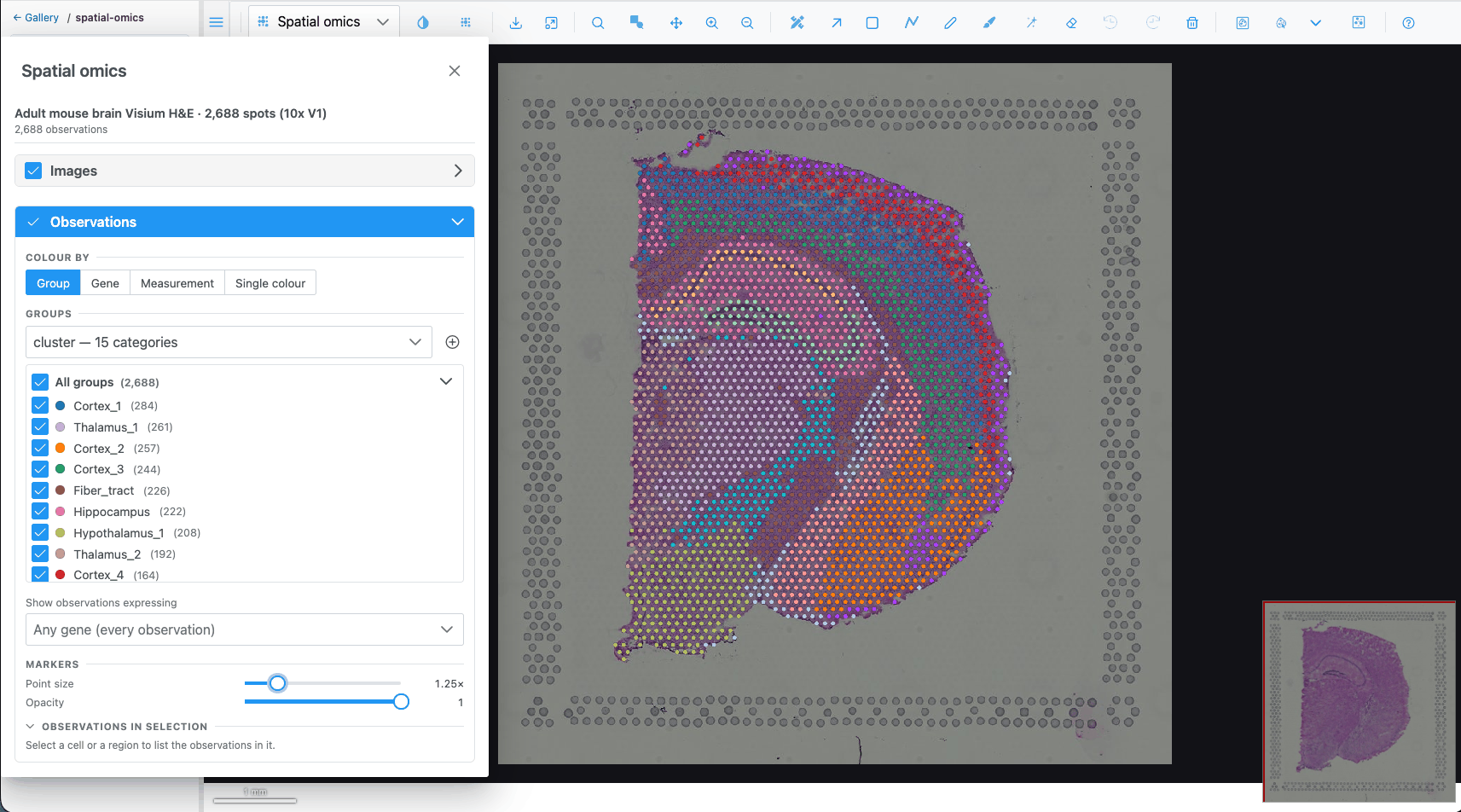
What you should see: one marker per Visium spot over the H&E image, coloured by the first group column (the clusters). The Spatial omics panel opens on the left; its header shows the dataset name and "2688 observations".
2. Colour by cluster
- In the panel, look at Observations → Colour by. Group is active, with the cluster column.
- Below it, the Groups list is the legend: one row per cluster with its colour and number of spots, largest first.
- Untick a cluster's checkbox. Its spots disappear from the map. Tick it again.
- Click a cluster's colour dot and pick another colour. The map updates.
- Click a cluster's name. Its spots are selected and every other spot is muted. Click the name again to clear the selection.
3. Colour by a gene
- Under Colour by, choose Gene.
- In the search box type
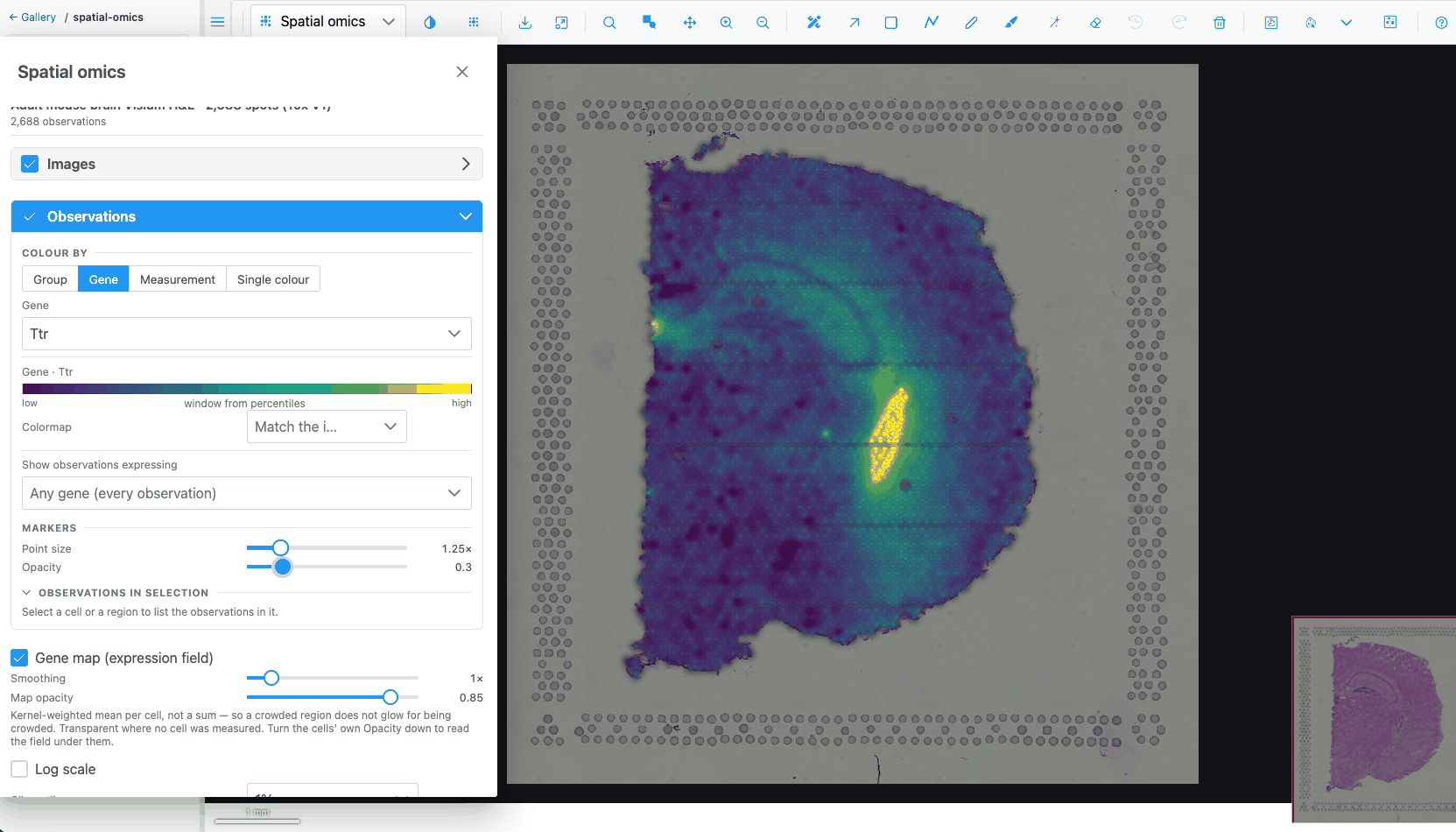
Ttrand pick it. Ttr is strongly expressed in the choroid plexus.
What you should see: spots coloured on a continuous scale, with a key showing the colour bar from low to high. Log scale may switch on by itself, because the dataset says its values are counts.
- Change Clip outliers from 1% to 5%. The colour window narrows, so mid-level spots stand out more.
- Pick a different scale in Colormap, for example Viridis. Clear it to go back to matching the image.
- Tick Gene map (expression field) and lower the markers' Opacity to about 0.3. A smooth estimate of the gene's expression is drawn under the spots.
- Untick Gene map and set Opacity back to 1.
4. Select spots with a region
- Switch Colour by back to Group.
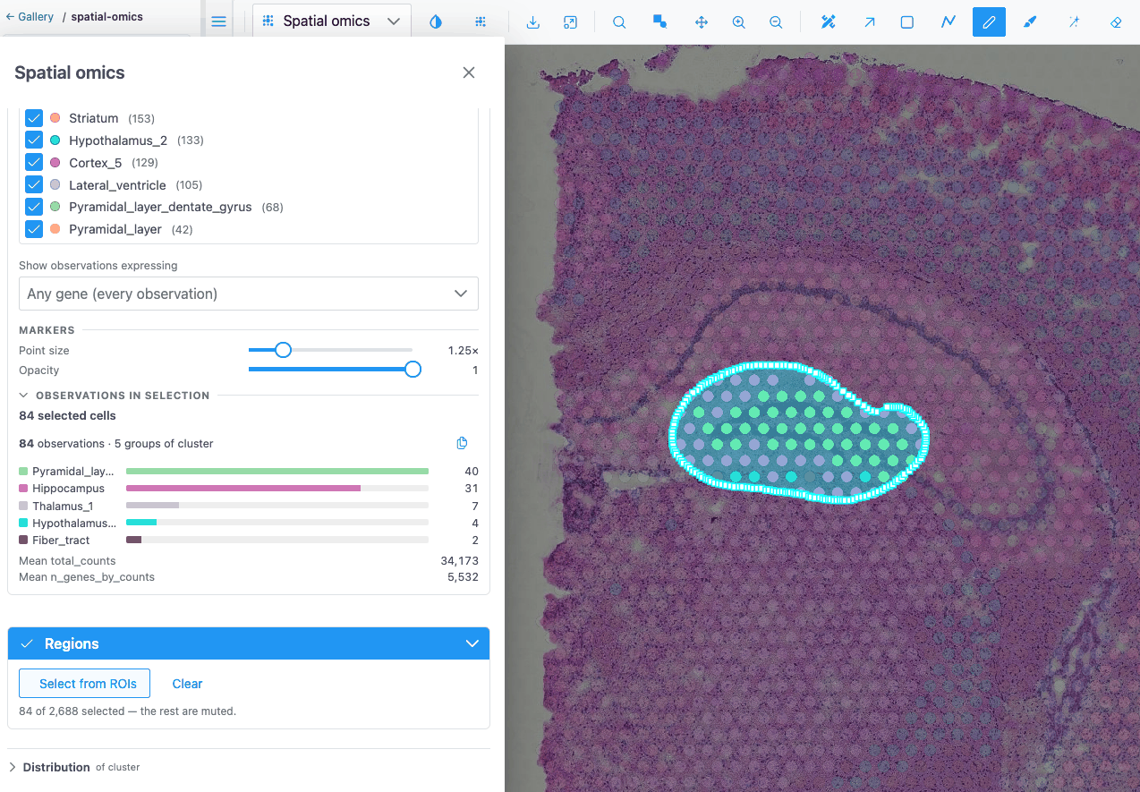
- Press F and draw a freeform region around one anatomical structure, for example the hippocampus.
- In the panel, expand Regions and click Select from ROIs.
What you should see: the spots inside your region stay bright and the others are muted. The hint reads "n of 2688 selected — the rest are muted". The Observations in selection summary lists how many spots of each cluster are inside.
Tip
Select from ROIs uses every region on the image, holes included, whichever tool drew it. The regions do not need to be visible: the Regions switch only shows or hides them.
5. Compare the selection with the whole section
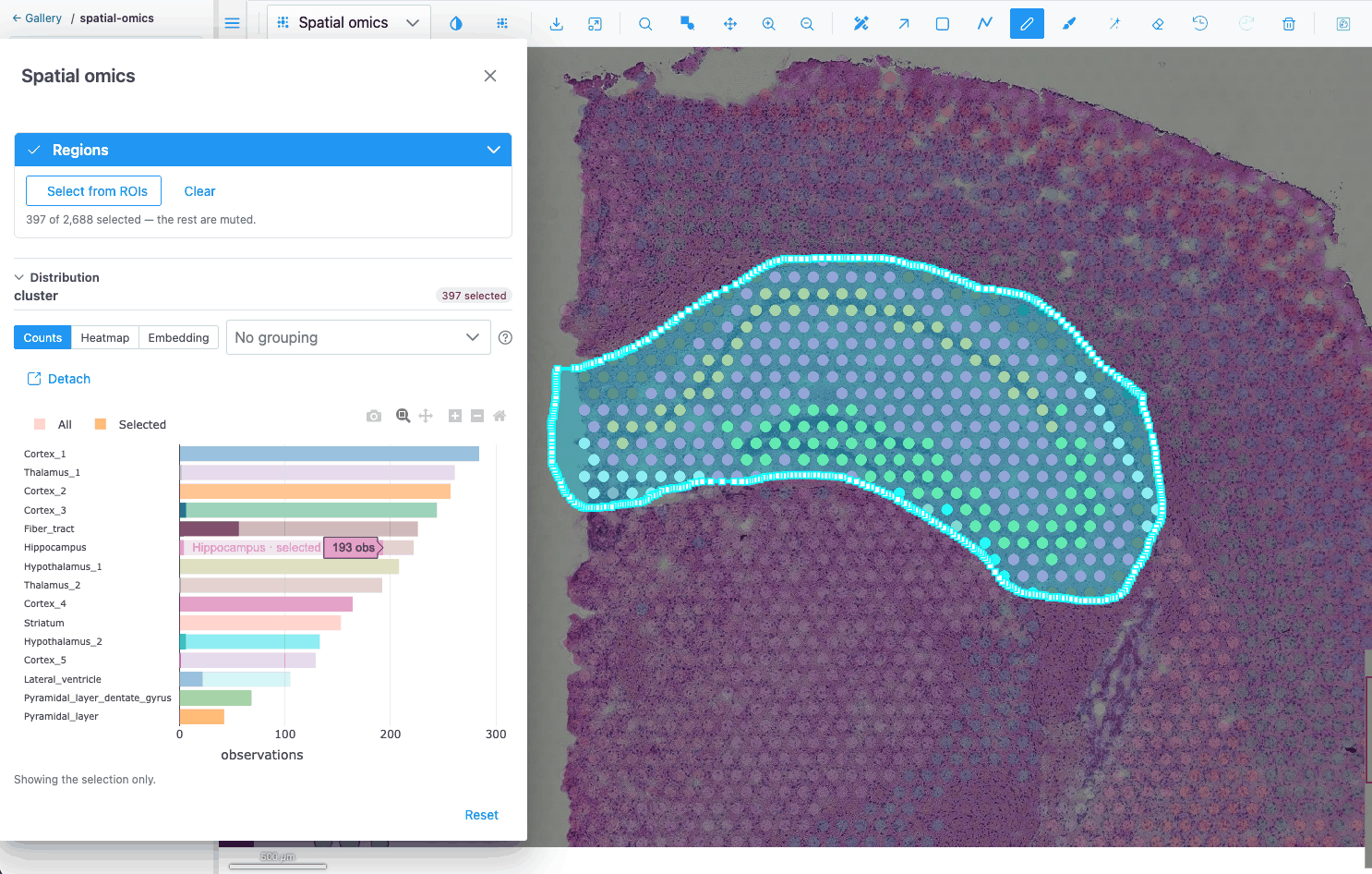
- Expand Distribution at the bottom of the panel. With a group colouring it shows Counts: the number of spots per cluster, with your selection drawn over the totals.
 2. Switch Colour by to Gene and pick
Ttr again. The chart switches to a Histogram of Ttr,
with the selection overlaid on the full distribution.
3. Choose Violin and set the grouping to cluster. You see Ttr's distribution in every cluster.
With a selection, only the selected spots are charted.
4. Choose Heatmap. Pick four or five genes in Pick genes for the rows, for example Ttr, Mbp,
Plp1, Nrgn and Hbb-bs. Each cell is the mean of a gene in a cluster, z-scored per gene by
default.
5. Click next to the chart tabs to read what the current chart shows,
and what it must not be read for.
6. Click Detach to move the chart into its own window next to the
map. Click Put back to return it.
Click Clear in the Regions section to clear the selection.
6. Select in an embedding
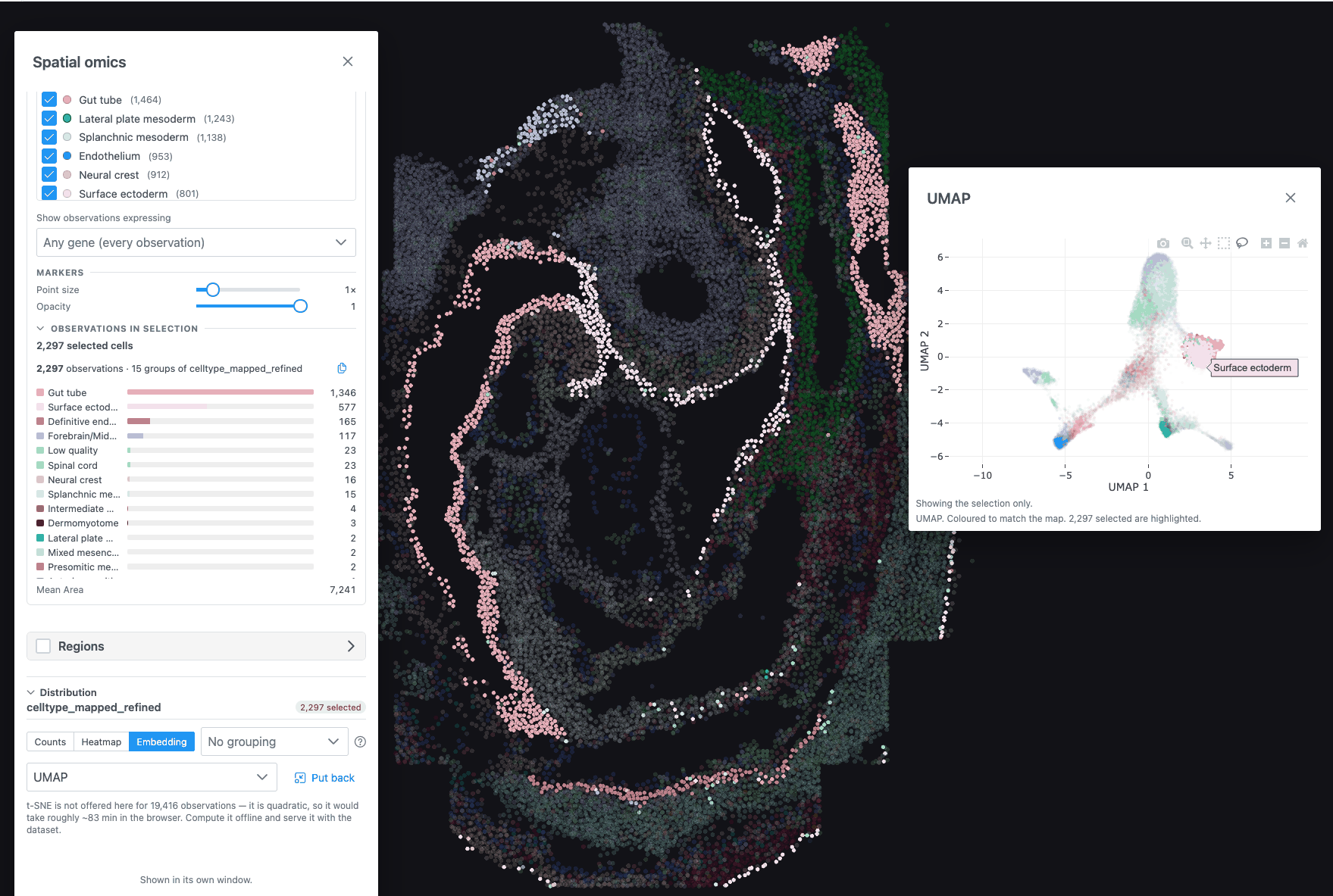
- Go back to the gallery's spatial-omics folder and open Mouse embryo seqFISH · 19,416 cells. It has no tissue image, so it opens directly in a spatial view.
- Open the Spatial omics panel. Under Colour by → Group, pick the cell-type column.
- In Distribution, choose Embedding and, if there is a choice, the UMAP.
- In the chart's toolbar choose the lasso, and draw around one cluster of points.
What you should see: the lassoed cells are highlighted on the map as well. The map and the embedding read the same selection.
7. A 3D atlas
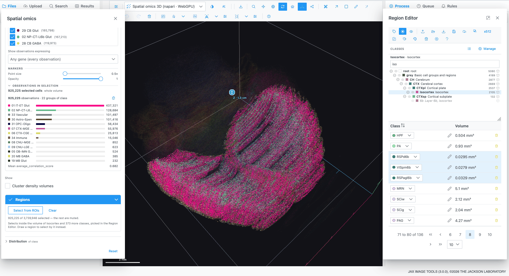
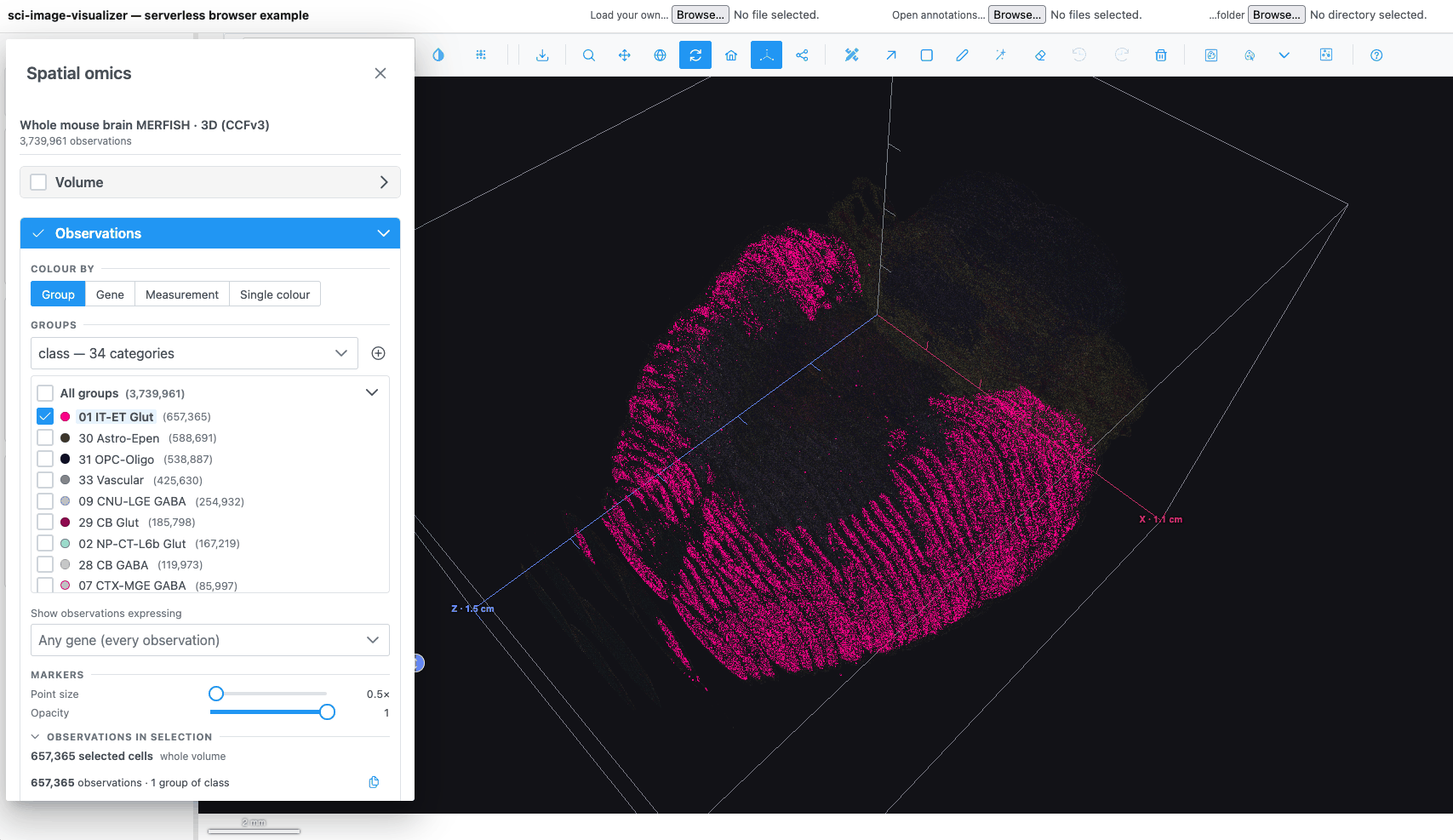
- Open spatial-omics → Allen Brain Cell Atlas → Whole mouse brain MERFISH · 3D · 1-in-10. The reference volume opens first in the Image view.
- Pick Spatial omics 3D in the plot-type dropdown. About 374,000 cells are drawn in 3D.
- Drag to rotate, scroll to zoom, and use Reset camera to start again.
- Load the atlas regions. Open the Region Editor, click Import regions
and choose two files together: the label volume
resampled_annotation.nii.gzand its ontologystructure_graph_1.json, both from the Allen Brain Cell Atlas download. In JAX Image Tools your administrator may have attached them already. - The Classes panel now shows the atlas's brain-region tree. Click a region, for example a cortical area, to pick it.
- In the Spatial omics panel, expand Regions and click Select from ROIs. The cells inside the picked region's volume are selected.
What you learned
- Opening a dataset and switching to the Spatial omics plot types.
- Colouring by group or gene, tuning the colour scale, and hiding or recolouring groups.
- Selecting observations from a drawn region, a group name, an embedding lasso or an atlas region.
- Reading the selection in Counts, Histogram, Violin, Heatmap and Embedding.
Next
- Spatial omics how-tos cover gene filters, importing cell groups and computing a t-SNE in the browser.
- The Spatial omics and Distribution charts reference pages describe every control.