DEG_analysis_BOT_vs_NTS
Last updated: 2024-01-06
Checks: 6 1
Knit directory: DO_Opioid/
This reproducible R Markdown analysis was created with workflowr (version 1.6.2). The Checks tab describes the reproducibility checks that were applied when the results were created. The Past versions tab lists the development history.
Great! Since the R Markdown file has been committed to the Git repository, you know the exact version of the code that produced these results.
Great job! The global environment was empty. Objects defined in the global environment can affect the analysis in your R Markdown file in unknown ways. For reproduciblity it’s best to always run the code in an empty environment.
The command set.seed(20200504) was run prior to running the code in the R Markdown file. Setting a seed ensures that any results that rely on randomness, e.g. subsampling or permutations, are reproducible.
Great job! Recording the operating system, R version, and package versions is critical for reproducibility.
Nice! There were no cached chunks for this analysis, so you can be confident that you successfully produced the results during this run.
Using absolute paths to the files within your workflowr project makes it difficult for you and others to run your code on a different machine. Change the absolute path(s) below to the suggested relative path(s) to make your code more reproducible.
| absolute | relative |
|---|---|
| /projects/compsci/vmp/USERS/heh/DO_Opioid/data/BOT_NTS_rnaseq_results/ | data/BOT_NTS_rnaseq_results |
Great! You are using Git for version control. Tracking code development and connecting the code version to the results is critical for reproducibility.
The results in this page were generated with repository version 6322cc6. See the Past versions tab to see a history of the changes made to the R Markdown and HTML files.
Note that you need to be careful to ensure that all relevant files for the analysis have been committed to Git prior to generating the results (you can use wflow_publish or wflow_git_commit). workflowr only checks the R Markdown file, but you know if there are other scripts or data files that it depends on. Below is the status of the Git repository when the results were generated:
Ignored files:
Ignored: .RData
Ignored: .Rhistory
Ignored: .Rproj.user/
Ignored: analysis/Picture1.png
Untracked files:
Untracked: Rplot_rz.png
Untracked: TIMBR.test.prop.bm.MN.RET.RData
Untracked: TIMBR.test.random.RData
Untracked: TIMBR.test.rz.transformed_TVb_ml.RData
Untracked: analysis/DDO_morphine1_second_set_69k.stdout
Untracked: analysis/DO_Fentanyl.R
Untracked: analysis/DO_Fentanyl.err
Untracked: analysis/DO_Fentanyl.out
Untracked: analysis/DO_Fentanyl.sh
Untracked: analysis/DO_Fentanyl_69k.R
Untracked: analysis/DO_Fentanyl_69k.err
Untracked: analysis/DO_Fentanyl_69k.out
Untracked: analysis/DO_Fentanyl_69k.sh
Untracked: analysis/DO_Fentanyl_Cohort2_GCTA_herit.R
Untracked: analysis/DO_Fentanyl_Cohort2_gemma.R
Untracked: analysis/DO_Fentanyl_Cohort2_mapping.R
Untracked: analysis/DO_Fentanyl_Cohort2_mapping.err
Untracked: analysis/DO_Fentanyl_Cohort2_mapping.out
Untracked: analysis/DO_Fentanyl_Cohort2_mapping.sh
Untracked: analysis/DO_Fentanyl_GCTA_herit.R
Untracked: analysis/DO_Fentanyl_alternate_metrics_69k.R
Untracked: analysis/DO_Fentanyl_alternate_metrics_69k.err
Untracked: analysis/DO_Fentanyl_alternate_metrics_69k.out
Untracked: analysis/DO_Fentanyl_alternate_metrics_69k.sh
Untracked: analysis/DO_Fentanyl_alternate_metrics_array.R
Untracked: analysis/DO_Fentanyl_alternate_metrics_array.err
Untracked: analysis/DO_Fentanyl_alternate_metrics_array.out
Untracked: analysis/DO_Fentanyl_alternate_metrics_array.sh
Untracked: analysis/DO_Fentanyl_array.R
Untracked: analysis/DO_Fentanyl_array.err
Untracked: analysis/DO_Fentanyl_array.out
Untracked: analysis/DO_Fentanyl_array.sh
Untracked: analysis/DO_Fentanyl_combining2Cohort_GCTA_herit.R
Untracked: analysis/DO_Fentanyl_combining2Cohort_gemma.R
Untracked: analysis/DO_Fentanyl_combining2Cohort_mapping.R
Untracked: analysis/DO_Fentanyl_combining2Cohort_mapping.err
Untracked: analysis/DO_Fentanyl_combining2Cohort_mapping.out
Untracked: analysis/DO_Fentanyl_combining2Cohort_mapping.sh
Untracked: analysis/DO_Fentanyl_combining2Cohort_mapping_CoxPH.R
Untracked: analysis/DO_Fentanyl_finalreport_to_plink.sh
Untracked: analysis/DO_Fentanyl_gemma.R
Untracked: analysis/DO_Fentanyl_gemma.err
Untracked: analysis/DO_Fentanyl_gemma.out
Untracked: analysis/DO_Fentanyl_gemma.sh
Untracked: analysis/DO_morphine1.R
Untracked: analysis/DO_morphine1.Rout
Untracked: analysis/DO_morphine1.sh
Untracked: analysis/DO_morphine1.stderr
Untracked: analysis/DO_morphine1.stdout
Untracked: analysis/DO_morphine1_SNP.R
Untracked: analysis/DO_morphine1_SNP.Rout
Untracked: analysis/DO_morphine1_SNP.sh
Untracked: analysis/DO_morphine1_SNP.stderr
Untracked: analysis/DO_morphine1_SNP.stdout
Untracked: analysis/DO_morphine1_combined.R
Untracked: analysis/DO_morphine1_combined.Rout
Untracked: analysis/DO_morphine1_combined.sh
Untracked: analysis/DO_morphine1_combined.stderr
Untracked: analysis/DO_morphine1_combined.stdout
Untracked: analysis/DO_morphine1_combined_69k.R
Untracked: analysis/DO_morphine1_combined_69k.Rout
Untracked: analysis/DO_morphine1_combined_69k.sh
Untracked: analysis/DO_morphine1_combined_69k.stderr
Untracked: analysis/DO_morphine1_combined_69k.stdout
Untracked: analysis/DO_morphine1_combined_69k_m2.R
Untracked: analysis/DO_morphine1_combined_69k_m2.Rout
Untracked: analysis/DO_morphine1_combined_69k_m2.sh
Untracked: analysis/DO_morphine1_combined_69k_m2.stderr
Untracked: analysis/DO_morphine1_combined_69k_m2.stdout
Untracked: analysis/DO_morphine1_combined_weight_DOB.R
Untracked: analysis/DO_morphine1_combined_weight_DOB.Rout
Untracked: analysis/DO_morphine1_combined_weight_DOB.err
Untracked: analysis/DO_morphine1_combined_weight_DOB.out
Untracked: analysis/DO_morphine1_combined_weight_DOB.sh
Untracked: analysis/DO_morphine1_combined_weight_DOB.stderr
Untracked: analysis/DO_morphine1_combined_weight_DOB.stdout
Untracked: analysis/DO_morphine1_combined_weight_age.R
Untracked: analysis/DO_morphine1_combined_weight_age.err
Untracked: analysis/DO_morphine1_combined_weight_age.out
Untracked: analysis/DO_morphine1_combined_weight_age.sh
Untracked: analysis/DO_morphine1_combined_weight_age_GAMMT.R
Untracked: analysis/DO_morphine1_combined_weight_age_GAMMT.err
Untracked: analysis/DO_morphine1_combined_weight_age_GAMMT.out
Untracked: analysis/DO_morphine1_combined_weight_age_GAMMT.sh
Untracked: analysis/DO_morphine1_combined_weight_age_GAMMT_chr19.R
Untracked: analysis/DO_morphine1_combined_weight_age_GAMMT_chr19.err
Untracked: analysis/DO_morphine1_combined_weight_age_GAMMT_chr19.out
Untracked: analysis/DO_morphine1_combined_weight_age_GAMMT_chr19.sh
Untracked: analysis/DO_morphine1_cph.R
Untracked: analysis/DO_morphine1_cph.Rout
Untracked: analysis/DO_morphine1_cph.sh
Untracked: analysis/DO_morphine1_second_set.R
Untracked: analysis/DO_morphine1_second_set.Rout
Untracked: analysis/DO_morphine1_second_set.sh
Untracked: analysis/DO_morphine1_second_set.stderr
Untracked: analysis/DO_morphine1_second_set.stdout
Untracked: analysis/DO_morphine1_second_set_69k.R
Untracked: analysis/DO_morphine1_second_set_69k.Rout
Untracked: analysis/DO_morphine1_second_set_69k.sh
Untracked: analysis/DO_morphine1_second_set_69k.stderr
Untracked: analysis/DO_morphine1_second_set_SNP.R
Untracked: analysis/DO_morphine1_second_set_SNP.Rout
Untracked: analysis/DO_morphine1_second_set_SNP.sh
Untracked: analysis/DO_morphine1_second_set_SNP.stderr
Untracked: analysis/DO_morphine1_second_set_SNP.stdout
Untracked: analysis/DO_morphine1_second_set_weight_DOB.R
Untracked: analysis/DO_morphine1_second_set_weight_DOB.Rout
Untracked: analysis/DO_morphine1_second_set_weight_DOB.err
Untracked: analysis/DO_morphine1_second_set_weight_DOB.out
Untracked: analysis/DO_morphine1_second_set_weight_DOB.sh
Untracked: analysis/DO_morphine1_second_set_weight_DOB.stderr
Untracked: analysis/DO_morphine1_second_set_weight_DOB.stdout
Untracked: analysis/DO_morphine1_second_set_weight_age.R
Untracked: analysis/DO_morphine1_second_set_weight_age.Rout
Untracked: analysis/DO_morphine1_second_set_weight_age.err
Untracked: analysis/DO_morphine1_second_set_weight_age.out
Untracked: analysis/DO_morphine1_second_set_weight_age.sh
Untracked: analysis/DO_morphine1_second_set_weight_age.stderr
Untracked: analysis/DO_morphine1_second_set_weight_age.stdout
Untracked: analysis/DO_morphine1_weight_DOB.R
Untracked: analysis/DO_morphine1_weight_DOB.sh
Untracked: analysis/DO_morphine1_weight_age.R
Untracked: analysis/DO_morphine1_weight_age.sh
Untracked: analysis/DO_morphine_gemma.R
Untracked: analysis/DO_morphine_gemma.err
Untracked: analysis/DO_morphine_gemma.out
Untracked: analysis/DO_morphine_gemma.sh
Untracked: analysis/DO_morphine_gemma_firstmin.R
Untracked: analysis/DO_morphine_gemma_firstmin.err
Untracked: analysis/DO_morphine_gemma_firstmin.out
Untracked: analysis/DO_morphine_gemma_firstmin.sh
Untracked: analysis/DO_morphine_gemma_withpermu.R
Untracked: analysis/DO_morphine_gemma_withpermu.err
Untracked: analysis/DO_morphine_gemma_withpermu.out
Untracked: analysis/DO_morphine_gemma_withpermu.sh
Untracked: analysis/DO_morphine_gemma_withpermu_firstbatch_min.depression.R
Untracked: analysis/DO_morphine_gemma_withpermu_firstbatch_min.depression.err
Untracked: analysis/DO_morphine_gemma_withpermu_firstbatch_min.depression.out
Untracked: analysis/DO_morphine_gemma_withpermu_firstbatch_min.depression.sh
Untracked: analysis/Lisa_Tarantino_Interval_needs_mvar_annotation.R
Untracked: analysis/Plot_DO_morphine1_SNP.R
Untracked: analysis/Plot_DO_morphine1_SNP.Rout
Untracked: analysis/Plot_DO_morphine1_SNP.sh
Untracked: analysis/Plot_DO_morphine1_SNP.stderr
Untracked: analysis/Plot_DO_morphine1_SNP.stdout
Untracked: analysis/Plot_DO_morphine1_second_set_SNP.R
Untracked: analysis/Plot_DO_morphine1_second_set_SNP.Rout
Untracked: analysis/Plot_DO_morphine1_second_set_SNP.sh
Untracked: analysis/Plot_DO_morphine1_second_set_SNP.stderr
Untracked: analysis/Plot_DO_morphine1_second_set_SNP.stdout
Untracked: analysis/download_GSE100356_sra.sh
Untracked: analysis/fentanyl_2cohorts_coxph.R
Untracked: analysis/fentanyl_2cohorts_coxph.err
Untracked: analysis/fentanyl_2cohorts_coxph.out
Untracked: analysis/fentanyl_2cohorts_coxph.sh
Untracked: analysis/fentanyl_scanone.cph.R
Untracked: analysis/fentanyl_scanone.cph.err
Untracked: analysis/fentanyl_scanone.cph.out
Untracked: analysis/fentanyl_scanone.cph.sh
Untracked: analysis/geo_rnaseq.R
Untracked: analysis/heritability_first_second_batch.R
Untracked: analysis/morphine_fentanyl_survival_time.R
Untracked: analysis/nf-rnaseq-b6.R
Untracked: analysis/plot_fentanyl_2cohorts_coxph.R
Untracked: analysis/scripts/
Untracked: analysis/tibmr.R
Untracked: analysis/timbr_demo.R
Untracked: analysis/workflow_proc.R
Untracked: analysis/workflow_proc.sh
Untracked: analysis/workflow_proc.stderr
Untracked: analysis/workflow_proc.stdout
Untracked: analysis/x.R
Untracked: analysis/~.sh
Untracked: code/PLINKtoCSVR.R
Untracked: code/cfw/
Untracked: code/gemma_plot.R
Untracked: code/process.sanger.snp.R
Untracked: code/reconst_utils.R
Untracked: data/69k_grid_pgmap.RData
Untracked: data/BOT_NTS_rnaseq_results/
Untracked: data/CC_SARS-1/
Untracked: data/CC_SARS-2/
Untracked: data/Composite Post Kevins Program Group 2 Fentanyl Prepped for Hao.xlsx
Untracked: data/DO_WBP_Data_JAB_to_map.xlsx
Untracked: data/Fentanyl_alternate_metrics.xlsx
Untracked: data/FinalReport/
Untracked: data/GM/
Untracked: data/GM_covar.csv
Untracked: data/GM_covar_07092018_morphine.csv
Untracked: data/Jackson_Lab_Bubier_MURGIGV01/
Untracked: data/Lisa Tarantino Interval needs mvar.xlsx
Untracked: data/Lisa_Tarantino_Interval_needs_mvar_annotation.csv
Untracked: data/MPD_Upload_October.csv
Untracked: data/MPD_Upload_October_updated_sex.csv
Untracked: data/Master Fentanyl DO Study Sheet.xlsx
Untracked: data/MasterMorphine Second Set DO w DOB2.xlsx
Untracked: data/MasterMorphine Second Set DO.xlsx
Untracked: data/Morphine CC DO mice Updated with Published inbred strains.csv
Untracked: data/Morphine_CC_DO_mice_Updated_with_Published_inbred_strains.csv
Untracked: data/cc_variants.sqlite
Untracked: data/combined/
Untracked: data/fentanyl/
Untracked: data/fentanyl2/
Untracked: data/fentanyl_1_2/
Untracked: data/fentanyl_2cohorts_coxph_data.Rdata
Untracked: data/first/
Untracked: data/founder_geno.csv
Untracked: data/genetic_map.csv
Untracked: data/gm.json
Untracked: data/gwas.sh
Untracked: data/marker_grid_0.02cM_plus.txt
Untracked: data/metabolomics_mouse_fecal/
Untracked: data/mouse_genes_mgi.sqlite
Untracked: data/pheno.csv
Untracked: data/pheno_qtl2.csv
Untracked: data/pheno_qtl2_07092018_morphine.csv
Untracked: data/pheno_qtl2_w_dob.csv
Untracked: data/physical_map.csv
Untracked: data/rnaseq/
Untracked: data/sample_geno.csv
Untracked: data/second/
Untracked: figure/
Untracked: glimma-plots/
Untracked: head.pdf
Untracked: output/DO_Fentanyl_Cohort2_MinDepressionRR_coefplot.pdf
Untracked: output/DO_Fentanyl_Cohort2_MinDepressionRR_coefplot_blup.pdf
Untracked: output/DO_Fentanyl_Cohort2_RRDepressionRateHrSLOPE_coefplot.pdf
Untracked: output/DO_Fentanyl_Cohort2_RRRecoveryRateHrSLOPE_coefplot.pdf
Untracked: output/DO_Fentanyl_Cohort2_RRRecoveryRateHrSLOPE_coefplot_blup.pdf
Untracked: output/DO_Fentanyl_Cohort2_StartofRecoveryHr_coefplot.pdf
Untracked: output/DO_Fentanyl_Cohort2_StartofRecoveryHr_coefplot_blup.pdf
Untracked: output/DO_Fentanyl_Cohort2_Statusbin_coefplot.pdf
Untracked: output/DO_Fentanyl_Cohort2_Statusbin_coefplot_blup.pdf
Untracked: output/DO_Fentanyl_Cohort2_SteadyStateDepressionDurationHrINTERVAL_coefplot.pdf
Untracked: output/DO_Fentanyl_Cohort2_TimetoDead(Hr)_coefplot.pdf
Untracked: output/DO_Fentanyl_Cohort2_TimetoDeadHr_coefplot.pdf
Untracked: output/DO_Fentanyl_Cohort2_TimetoDeadHr_coefplot_blup.pdf
Untracked: output/DO_Fentanyl_Cohort2_TimetoProjectedRecoveryHr_coefplot.pdf
Untracked: output/DO_Fentanyl_Cohort2_TimetoProjectedRecoveryHr_coefplot_blup.pdf
Untracked: output/DO_Fentanyl_Cohort2_TimetoSteadyRRDepression(Hr)_coefplot.pdf
Untracked: output/DO_Fentanyl_Cohort2_TimetoSteadyRRDepressionHr_coefplot.pdf
Untracked: output/DO_Fentanyl_Cohort2_TimetoSteadyRRDepressionHr_coefplot_blup.pdf
Untracked: output/DO_Fentanyl_Cohort2_TimetoThresholdRecoveryHr_coefplot.pdf
Untracked: output/DO_Fentanyl_Cohort2_TimetoThresholdRecoveryHr_coefplot_blup.pdf
Untracked: output/DO_morphine_Min.depression.png
Untracked: output/DO_morphine_Min.depression22222_violin_chr5.pdf
Untracked: output/DO_morphine_Min.depression_coefplot.pdf
Untracked: output/DO_morphine_Min.depression_coefplot_blup.pdf
Untracked: output/DO_morphine_Min.depression_coefplot_blup_chr5.png
Untracked: output/DO_morphine_Min.depression_coefplot_blup_chrX.png
Untracked: output/DO_morphine_Min.depression_coefplot_chr5.png
Untracked: output/DO_morphine_Min.depression_coefplot_chrX.png
Untracked: output/DO_morphine_Min.depression_peak_genes_chr5.png
Untracked: output/DO_morphine_Min.depression_violin_chr5.png
Untracked: output/DO_morphine_Recovery.Time.png
Untracked: output/DO_morphine_Recovery.Time_coefplot.pdf
Untracked: output/DO_morphine_Recovery.Time_coefplot_blup.pdf
Untracked: output/DO_morphine_Recovery.Time_coefplot_blup_chr11.png
Untracked: output/DO_morphine_Recovery.Time_coefplot_blup_chr4.png
Untracked: output/DO_morphine_Recovery.Time_coefplot_blup_chr7.png
Untracked: output/DO_morphine_Recovery.Time_coefplot_blup_chr9.png
Untracked: output/DO_morphine_Recovery.Time_coefplot_chr11.png
Untracked: output/DO_morphine_Recovery.Time_coefplot_chr4.png
Untracked: output/DO_morphine_Recovery.Time_coefplot_chr7.png
Untracked: output/DO_morphine_Recovery.Time_coefplot_chr9.png
Untracked: output/DO_morphine_Status_bin.png
Untracked: output/DO_morphine_Status_bin_coefplot.pdf
Untracked: output/DO_morphine_Status_bin_coefplot_blup.pdf
Untracked: output/DO_morphine_Survival.Time.png
Untracked: output/DO_morphine_Survival.Time_coefplot.pdf
Untracked: output/DO_morphine_Survival.Time_coefplot_blup.pdf
Untracked: output/DO_morphine_Survival.Time_coefplot_blup_chr17.png
Untracked: output/DO_morphine_Survival.Time_coefplot_blup_chr8.png
Untracked: output/DO_morphine_Survival.Time_coefplot_chr17.png
Untracked: output/DO_morphine_Survival.Time_coefplot_chr8.png
Untracked: output/DO_morphine_combine_batch_peak_violin.pdf
Untracked: output/DO_morphine_combined_69k_m2_Min.depression.png
Untracked: output/DO_morphine_combined_69k_m2_Min.depression_coefplot.pdf
Untracked: output/DO_morphine_combined_69k_m2_Min.depression_coefplot_blup.pdf
Untracked: output/DO_morphine_combined_69k_m2_Recovery.Time.png
Untracked: output/DO_morphine_combined_69k_m2_Recovery.Time_coefplot.pdf
Untracked: output/DO_morphine_combined_69k_m2_Recovery.Time_coefplot_blup.pdf
Untracked: output/DO_morphine_combined_69k_m2_Status_bin.png
Untracked: output/DO_morphine_combined_69k_m2_Status_bin_coefplot.pdf
Untracked: output/DO_morphine_combined_69k_m2_Status_bin_coefplot_blup.pdf
Untracked: output/DO_morphine_combined_69k_m2_Survival.Time.png
Untracked: output/DO_morphine_combined_69k_m2_Survival.Time_coefplot.pdf
Untracked: output/DO_morphine_combined_69k_m2_Survival.Time_coefplot_blup.pdf
Untracked: output/DO_morphine_coxph_24hrs_kinship_QTL.png
Untracked: output/DO_morphine_cphout.RData
Untracked: output/DO_morphine_first_batch_peak_in_second_batch_violin.pdf
Untracked: output/DO_morphine_first_batch_peak_in_second_batch_violin_sidebyside.pdf
Untracked: output/DO_morphine_first_batch_peak_violin.pdf
Untracked: output/DO_morphine_operm.cph.RData
Untracked: output/DO_morphine_second_batch_on_first_batch_peak_violin.pdf
Untracked: output/DO_morphine_second_batch_peak_ch6surv_on_first_batchviolin.pdf
Untracked: output/DO_morphine_second_batch_peak_ch6surv_on_first_batchviolin2.pdf
Untracked: output/DO_morphine_second_batch_peak_in_first_batch_violin.pdf
Untracked: output/DO_morphine_second_batch_peak_in_first_batch_violin_sidebyside.pdf
Untracked: output/DO_morphine_second_batch_peak_violin.pdf
Untracked: output/DO_morphine_secondbatch_69k_Min.depression.png
Untracked: output/DO_morphine_secondbatch_69k_Min.depression_coefplot.pdf
Untracked: output/DO_morphine_secondbatch_69k_Min.depression_coefplot_blup.pdf
Untracked: output/DO_morphine_secondbatch_69k_Recovery.Time.png
Untracked: output/DO_morphine_secondbatch_69k_Recovery.Time_coefplot.pdf
Untracked: output/DO_morphine_secondbatch_69k_Recovery.Time_coefplot_blup.pdf
Untracked: output/DO_morphine_secondbatch_69k_Status_bin.png
Untracked: output/DO_morphine_secondbatch_69k_Status_bin_coefplot.pdf
Untracked: output/DO_morphine_secondbatch_69k_Status_bin_coefplot_blup.pdf
Untracked: output/DO_morphine_secondbatch_69k_Survival.Time.png
Untracked: output/DO_morphine_secondbatch_69k_Survival.Time_coefplot.pdf
Untracked: output/DO_morphine_secondbatch_69k_Survival.Time_coefplot_blup.pdf
Untracked: output/DO_morphine_secondbatch_Min.depression.png
Untracked: output/DO_morphine_secondbatch_Min.depression_coefplot.pdf
Untracked: output/DO_morphine_secondbatch_Min.depression_coefplot_blup.pdf
Untracked: output/DO_morphine_secondbatch_Recovery.Time.png
Untracked: output/DO_morphine_secondbatch_Recovery.Time_coefplot.pdf
Untracked: output/DO_morphine_secondbatch_Recovery.Time_coefplot_blup.pdf
Untracked: output/DO_morphine_secondbatch_Status_bin.png
Untracked: output/DO_morphine_secondbatch_Status_bin_coefplot.pdf
Untracked: output/DO_morphine_secondbatch_Status_bin_coefplot_blup.pdf
Untracked: output/DO_morphine_secondbatch_Survival.Time.png
Untracked: output/DO_morphine_secondbatch_Survival.Time_coefplot.pdf
Untracked: output/DO_morphine_secondbatch_Survival.Time_coefplot_blup.pdf
Untracked: output/Fentanyl/
Untracked: output/KPNA3.pdf
Untracked: output/SSC4D.pdf
Untracked: output/TIMBR.test.RData
Untracked: output/apr_69kchr_combined.RData
Untracked: output/apr_69kchr_k_loco_combined.rds
Untracked: output/apr_69kchr_second_set.RData
Untracked: output/combine_batch_variation.RData
Untracked: output/combined_gm.RData
Untracked: output/combined_gm.k_loco.rds
Untracked: output/combined_gm.k_overall.rds
Untracked: output/combined_gm.probs_8state.rds
Untracked: output/coxph/
Untracked: output/do.morphine.RData
Untracked: output/do.morphine.k_loco.rds
Untracked: output/do.morphine.probs_36state.rds
Untracked: output/do.morphine.probs_8state.rds
Untracked: output/do_Fentanyl_combine2cohort_MeanDepressionBR_coefplot.pdf
Untracked: output/do_Fentanyl_combine2cohort_MeanDepressionBR_coefplot_blup.pdf
Untracked: output/do_Fentanyl_combine2cohort_MinDepressionBR_coefplot.pdf
Untracked: output/do_Fentanyl_combine2cohort_MinDepressionBR_coefplot_blup.pdf
Untracked: output/do_Fentanyl_combine2cohort_MinDepressionRR_coefplot.pdf
Untracked: output/do_Fentanyl_combine2cohort_MinDepressionRR_coefplot_blup.pdf
Untracked: output/do_Fentanyl_combine2cohort_RRRecoveryRateHr_coefplot.pdf
Untracked: output/do_Fentanyl_combine2cohort_RRRecoveryRateHr_coefplot_blup.pdf
Untracked: output/do_Fentanyl_combine2cohort_StartofRecoveryHr_coefplot.pdf
Untracked: output/do_Fentanyl_combine2cohort_StartofRecoveryHr_coefplot_blup.pdf
Untracked: output/do_Fentanyl_combine2cohort_Statusbin_coefplot.pdf
Untracked: output/do_Fentanyl_combine2cohort_Statusbin_coefplot_blup.pdf
Untracked: output/do_Fentanyl_combine2cohort_SteadyStateDepressionDurationHr_coefplot.pdf
Untracked: output/do_Fentanyl_combine2cohort_SteadyStateDepressionDurationHr_coefplot_blup.pdf
Untracked: output/do_Fentanyl_combine2cohort_SurvivalTime_coefplot.pdf
Untracked: output/do_Fentanyl_combine2cohort_SurvivalTime_coefplot_blup.pdf
Untracked: output/do_Fentanyl_combine2cohort_TimetoDeadHr_coefplot.pdf
Untracked: output/do_Fentanyl_combine2cohort_TimetoDeadHr_coefplot_blup.pdf
Untracked: output/do_Fentanyl_combine2cohort_TimetoMostlyDeadHr_coefplot.pdf
Untracked: output/do_Fentanyl_combine2cohort_TimetoMostlyDeadHr_coefplot_blup.pdf
Untracked: output/do_Fentanyl_combine2cohort_TimetoProjectedRecoveryHr_coefplot.pdf
Untracked: output/do_Fentanyl_combine2cohort_TimetoProjectedRecoveryHr_coefplot_blup.pdf
Untracked: output/do_Fentanyl_combine2cohort_TimetoRecoveryHr_coefplot.pdf
Untracked: output/do_Fentanyl_combine2cohort_TimetoRecoveryHr_coefplot_blup.pdf
Untracked: output/first_batch_variation.RData
Untracked: output/first_second_survival_peak_chr.xlsx
Untracked: output/hsq_1_first_batch_herit_qtl2.RData
Untracked: output/hsq_2_second_batch_herit_qtl2.RData
Untracked: output/morphine_fentanyl_survival_time.pdf
Untracked: output/old_temp/
Untracked: output/out_1_operm.RData
Untracked: output/pr_69kchr_combined.RData
Untracked: output/pr_69kchr_second_set.RData
Untracked: output/qtl.morphine.69k.out.combined.RData
Untracked: output/qtl.morphine.69k.out.combined_m2.RData
Untracked: output/qtl.morphine.69k.out.second_set.RData
Untracked: output/qtl.morphine.operm.RData
Untracked: output/qtl.morphine.out.RData
Untracked: output/qtl.morphine.out.combined_gm.RData
Untracked: output/qtl.morphine.out.combined_gm.female.RData
Untracked: output/qtl.morphine.out.combined_gm.male.RData
Untracked: output/qtl.morphine.out.combined_weight_DOB.RData
Untracked: output/qtl.morphine.out.combined_weight_age.RData
Untracked: output/qtl.morphine.out.female.RData
Untracked: output/qtl.morphine.out.male.RData
Untracked: output/qtl.morphine.out.second_set.RData
Untracked: output/qtl.morphine.out.second_set.female.RData
Untracked: output/qtl.morphine.out.second_set.male.RData
Untracked: output/qtl.morphine.out.second_set.weight_DOB.RData
Untracked: output/qtl.morphine.out.second_set.weight_age.RData
Untracked: output/qtl.morphine.out.weight_DOB.RData
Untracked: output/qtl.morphine.out.weight_age.RData
Untracked: output/qtl.morphine1.snpout.RData
Untracked: output/qtl.morphine2.snpout.RData
Untracked: output/sample_all_infor.csv
Untracked: output/sample_all_infor.txt
Untracked: output/second_batch_pheno.csv
Untracked: output/second_batch_variation.RData
Untracked: output/second_set_apr_69kchr_k_loco.rds
Untracked: output/second_set_gm.RData
Untracked: output/second_set_gm.k_loco.rds
Untracked: output/second_set_gm.probs_36state.rds
Untracked: output/second_set_gm.probs_8state.rds
Untracked: output/topSNP_chr5_mindepression.csv
Untracked: output/zoompeak_Min.depression_9.pdf
Untracked: output/zoompeak_Recovery.Time_16.pdf
Untracked: output/zoompeak_Status_bin_11.pdf
Untracked: output/zoompeak_Survival.Time_1.pdf
Untracked: output/zoompeak_fentanyl_Survival.Time_2.pdf
Untracked: sra-tools_v2.10.7.sif
Unstaged changes:
Modified: .gitignore
Modified: _workflowr.yml
Deleted: analysis/CC_SARS-2.Rmd
Modified: analysis/CC_SARS.Rmd
Modified: analysis/marker_violin.Rmd
Modified: output/CC_SARS_Chr16_QTL_interval.pdf
Modified: output/CC_SARS_Chr16_plotGeno.pdf
Modified: output/CC_SARS_Chr16_plotGeno.png
Note that any generated files, e.g. HTML, png, CSS, etc., are not included in this status report because it is ok for generated content to have uncommitted changes.
These are the previous versions of the repository in which changes were made to the R Markdown (analysis/DEG_analysis_BOT_vs_NTS.Rmd) and HTML (docs/DEG_analysis_BOT_vs_NTS.html) files. If you’ve configured a remote Git repository (see ?wflow_git_remote), click on the hyperlinks in the table below to view the files as they were in that past version.
| File | Version | Author | Date | Message |
|---|---|---|---|---|
| Rmd | 6322cc6 | xhyuo | 2024-01-06 | pc2 |
| html | acb1314 | xhyuo | 2023-12-23 | Build site. |
| Rmd | 883216f | xhyuo | 2023-12-23 | Sex DEG in tissue |
| html | 2cc8a55 | xhyuo | 2023-12-11 | Build site. |
| Rmd | 16d2e1c | xhyuo | 2023-12-11 | wgcna trait r2 no color |
| html | 85a6803 | xhyuo | 2023-12-04 | Build site. |
| Rmd | 892396d | xhyuo | 2023-12-03 | wgcna trait r2 |
| html | 52c098c | xhyuo | 2023-11-28 | Build site. |
| Rmd | 3d209a0 | xhyuo | 2023-11-28 | wgcna hub gene |
| html | b48269e | xhyuo | 2023-11-09 | Build site. |
| Rmd | bfbbb27 | xhyuo | 2023-11-09 | wgcna no head table |
| html | 5424b39 | xhyuo | 2023-11-06 | Build site. |
| Rmd | 034786a | xhyuo | 2023-11-06 | wgcna |
| html | 46f2f59 | xhyuo | 2023-10-20 | Build site. |
| Rmd | 5cc0eb1 | xhyuo | 2023-10-20 | DEG_analysis_BOT_vs_NTS 3 missings |
| html | b24fa56 | xhyuo | 2023-10-17 | Build site. |
| Rmd | c6aa7b3 | xhyuo | 2023-10-17 | DEG_analysis_BOT_vs_NTS |
workflow for rna-seq samples
library
library(stringr)
library(tidyverse)Warning: replacing previous import 'lifecycle::last_warnings' by
'rlang::last_warnings' when loading 'hms'Warning: replacing previous import 'ellipsis::check_dots_unnamed' by
'rlang::check_dots_unnamed' when loading 'hms'Warning: replacing previous import 'ellipsis::check_dots_used' by
'rlang::check_dots_used' when loading 'hms'Warning: replacing previous import 'ellipsis::check_dots_empty' by
'rlang::check_dots_empty' when loading 'hms'Warning: package 'purrr' was built under R version 4.0.5library(edgeR)
library(limma)
library(Glimma)
library(gplots)
library(org.Mm.eg.db)
library(RColorBrewer)
library(DESeq2)
library(pheatmap)
library(ggrepel)
library(DT)
library(enrichR)
library(cowplot)
library(ggplotify)
library(data.table)
library(WGCNA)
library(grid)
set.seed(123)Collect RNA-seq emase out on gene level abundances.
#define the output directory
####merge all the genes.expected_read_counts####
all.dgerc.file <- list.files(path = "/projects/compsci/vmp/USERS/heh/DO_Opioid/data/BOT_NTS_rnaseq_results/",
pattern = "\\.multiway.genes.expected_read_counts$",
full.names = FALSE,
all.files = TRUE,
recursive = TRUE)
all.dgerc.file <- all.dgerc.file[!str_detect(all.dgerc.file, "Undetermined")]
#get the sample id
sampleid <- gsub(".*/", "", all.dgerc.file)
sampleid <- str_extract(sampleid, "^[^_]+_[^_]+")
#BOT
BOT_sample <- map_dfr(
c("/projects/activities/bubier/rnaseq/fastq/20230707_23-chesler-001/23-chesler-001_QCreport.csv","/projects/activities/bubier/rnaseq/fastq/20230710_23-chesler-001-run2/23-chesler-001-run2_QCreport.csv"), function(x){
read_csv(x, skip = 16) %>%
dplyr::mutate(folder = x)
}) %>%
dplyr::mutate(id = str_extract(Sample_Name, "^[^_]+_[^_]+"),
.before = 1)
#NTS
NTS_sample <- map2_dfr(
c("/projects/activities/bubier/rnaseq/fastq/20230710_23-chesler-002/23-chesler-002_QCreport.csv",
"/projects/activities/bubier/rnaseq/fastq/20230717_23-chesler-002-run2/23-chesler-002-run2_QCreport.csv",
"/projects/activities/bubier/rnaseq/fastq/20230721_23-chesler-002-run3/23-chesler-002-run3_QCreport.csv",
"/projects/activities/bubier/rnaseq/fastq/20230807_23-chesler-002-run4/23-chesler-002-run4_QCreport.csv"),
c(16,16,16,17),
function(x,y){
read_csv(x, skip = y) %>%
dplyr::mutate(folder = x)
}) %>%
dplyr::mutate(id = str_extract(Sample_Name, "^[^_]+_[^_]+"),
.before = 1)
#merge
BOT_NTS_sample <- bind_rows(BOT_sample, NTS_sample, .id = "Tissue") %>%
dplyr::mutate(Tissue = if_else(Tissue==1, "BOT", "NTS")) %>%
dplyr::filter(id %in% sampleid)
sheet <- readxl::read_excel("data/BOT_NTS_rnaseq_results/Bubier Brain Tracking Sheet.xlsx", sheet = 1, col_types = c("text", "text", "text", "numeric", "date", "logical", "text", "text", "text", "text", "text"), range = "A1:K393") %>%
dplyr::select(1,2,3,5) %>%
dplyr::distinct()
#data.frame
all.dgerc <- data.frame(file = all.dgerc.file, sampleid = sampleid) %>%
dplyr::left_join(BOT_NTS_sample, by = c("sampleid" = "id")) %>%
dplyr::mutate(id = gsub("\\_GT23.*","",sampleid)) %>%
dplyr::left_join(sheet, by = c("id" = "JCMS #")) %>%
dplyr::group_by(sampleid, Tissue) %>%
dplyr::slice_max(Reads_Total) %>%
dplyr::ungroup()
#39735
all.dgerc$Sex[all.dgerc$id == 39735] = c("F", "F")
all.dgerc$`Strain Name`[all.dgerc$id == 39735] = c("CC019/TauUncJ", "CC019/TauUncJ")
#40042
all.dgerc$Sex[all.dgerc$id == 40042] = c("M", "M")
all.dgerc$`Strain Name`[all.dgerc$id == 40042] = c("CC013/GeniUncJ", "CC013/GeniUncJ")
#40043
all.dgerc$Sex[all.dgerc$id == 40043] = "M"
all.dgerc$`Strain Name`[all.dgerc$id == 40043] = "CC013/GeniUncJ"
#merge
command.merge.dgerc <- paste0("bash -c 'paste ", paste(paste0("<(cut -f 10 /projects/compsci/vmp/USERS/heh/DO_Opioid/data/BOT_NTS_rnaseq_results/", all.dgerc.file,")"), collapse = " "), " > /projects/compsci/vmp/USERS/heh/DO_Opioid/data/BOT_NTS_rnaseq_results/merged.dgerc2'")
system(command.merge.dgerc)
#read into R
merged.dgerc <- read.table("data/BOT_NTS_rnaseq_results/merged.dgerc2", header = T, sep = "\t")
colnames(merged.dgerc) <- sampleid
expgene <- read.table(file = paste0("data/BOT_NTS_rnaseq_results/",as.character(all.dgerc$file[1])),header=TRUE,sep="\t")
rownames(merged.dgerc) <- expgene[,1]
write.csv(merged.dgerc,file="data/BOT_NTS_rnaseq_results/merged.dgerc2.csv",quote=F,row.names=T)
save(merged.dgerc, file="data/BOT_NTS_rnaseq_results/merged.dgerc2.RData")
save(all.dgerc, file="data/BOT_NTS_rnaseq_results/all.dgerc2.RData")count matrix and design matrix
log1 = readxl::read_excel("data/BOT_NTS_rnaseq_results/23-chesler-001_RNA_Project_Log_v2-2023.xlsx",
sheet = 1, skip = 1) %>%
dplyr::select(-1) %>%
dplyr::slice(-199:-200)New names:
* `Notes/Comments` -> `Notes/Comments...20`
* `Notes/Comments` -> `Notes/Comments...21`log2 = readxl::read_excel("data/BOT_NTS_rnaseq_results/23-chesler-002_RNA_Project_Log_v2_07-24-2023.xlsx",
sheet = 1, skip = 1) %>%
dplyr::select(-1) %>%
dplyr::slice(-199:-200)
log = bind_rows(log1, log2, .id = "Run")New names:
* `Notes/Comments...20` -> `Notes/Comments...19`
* `Notes/Comments...21` -> `Notes/Comments...20`log = log %>%
dplyr::mutate(sampleid = paste0(log$`Customer Sample Name`, "_", log$`GT Sample Name`), .before = 1)
load("data/BOT_NTS_rnaseq_results/all.dgerc2.RData")
#RNA seq count data
countdata <- get(load("data/BOT_NTS_rnaseq_results/merged.dgerc2.RData"))
#floor countdata
countdata <- floor(countdata)
#Removing genes that are lowly expressed as 0
countdata <- countdata[rowSums(countdata) != 0,]
#gene annotation
genes <- AnnotationDbi::select(org.Mm.eg.db, keys=rownames(countdata), columns=c("SYMBOL"),
keytype="ENSEMBL")'select()' returned 1:many mapping between keys and columnsgenes <- genes[!duplicated(genes$ENSEMBL),]
genes <- genes[match(rownames(countdata), genes$ENSEMBL),]
#order
all.equal(rownames(countdata), genes$ENSEMBL)[1] TRUE#"35714_NTS_M" "38604_NTS_M" "38663_NTS_M" "40073_NTS_M"
#design matrix
design.matrix <- all.dgerc %>%
#dplyr::select(-1) %>%
dplyr::rename(Strain = 24) %>%
dplyr::mutate(name = case_when(
id %in% c(35714, 38604, 38663, 40073) ~ paste(all.dgerc$sampleid, all.dgerc$Tissue, all.dgerc$Sex, sep = "_"),
TRUE ~ paste(all.dgerc$id, all.dgerc$Tissue, all.dgerc$Sex, sep = "_")
)) %>%
group_by(name) %>%
dplyr::mutate(name = make.unique(as.character(name))) %>%
dplyr::mutate(across(c(Sex, Strain, Tissue), as.factor))
rownames(design.matrix) = design.matrix$nameWarning: Setting row names on a tibble is deprecated.#strain_means
#strain_means = read_csv("data/BOT_NTS_rnaseq_results/MPD_Project/Project1046_strainmeans.csv")
strain_means = map_dfr(c("data/BOT_NTS_rnaseq_results/MPD_Project/Project1046_strainmeans.csv",
"data/BOT_NTS_rnaseq_results/MPD_Project/Project1047_strainmeans.csv",
"data/BOT_NTS_rnaseq_results/MPD_Project/Project1167_strainmeans.csv"),
~read.csv(.x))
strain_means_wide = strain_means %>%
dplyr::select(2,3,5,6) %>%
#dplyr::filter(str_detect(varname, "Baseline|Time|Depression|Recovery")) %>%
dplyr::filter(!str_detect(varname, "WEIGHT|STATUS|Mouse|AGE")) %>%
tidyr::pivot_wider(names_from = varname, values_from = mean) %>%
dplyr::rename(Strain = strain, Sex = sex) %>%
dplyr::mutate(Sex = toupper(Sex))
#left_join
design.matrix.pheno = design.matrix %>%
left_join(strain_means_wide) %>%
dplyr::select(where(~ !all(is.na(.)))) %>%
as.data.frame()Joining, by = c("Sex", "Strain")rownames(design.matrix.pheno) = design.matrix.pheno$name
#design.matrix$group <- factor(paste0(design.matrix$Strain, design.matrix$Tissue))
#order
all.equal(design.matrix$sampleid, colnames(countdata))[1] TRUE#new colname of countdata
colnames(countdata) = rownames(design.matrix)
#To now construct the DESeqDataSet object from the matrix of counts and the sample information table, we use:
ddsMat <- DESeqDataSetFromMatrix(countData = countdata,
colData = design.matrix,
design = ~Strain + Tissue + Sex)converting counts to integer mode Note: levels of factors in the design contain characters other than
letters, numbers, '_' and '.'. It is recommended (but not required) to use
only letters, numbers, and delimiters '_' or '.', as these are safe characters
for column names in R. [This is a message, not a warning or an error]QC process
#Pre-filtering the dataset
#perform a minimal pre-filtering to keep only rows that have at least 10 reads total.
keep <- rowSums(counts(ddsMat) >= 10) >= 2
ddsMat <- ddsMat[keep,]
ddsMatclass: DESeqDataSet
dim: 21651 380
metadata(1): version
assays(1): counts
rownames(21651): ENSMUSG00000000001 ENSMUSG00000000028 ...
ENSMUSG00001074846 ENSMUSG00002076083
rowData names(0):
colnames(380): 34303_BOT_F 34303_NTS_F ... 41415_BOT_F 41415_NTS_F
colData names(26): file sampleid ... DOB namenrow(ddsMat)[1] 21651## [1] 21651
# DESeq2 creates a matrix when you use the counts() function
## First convert normalized_counts to a data frame and transfer the row names to a new column called "gene"
# this gives log2(n + 1)
ntd <- normTransform(ddsMat) Note: levels of factors in the design contain characters other than
letters, numbers, '_' and '.'. It is recommended (but not required) to use
only letters, numbers, and delimiters '_' or '.', as these are safe characters
for column names in R. [This is a message, not a warning or an error]normalized_counts <- assay(ntd) %>%
data.frame() %>%
rownames_to_column(var="gene") %>%
as_tibble()
#The variance stabilizing transformation and the rlog
#The rlog tends to work well on small datasets (n < 30), potentially outperforming the VST when there is a wide range of sequencing depth across samples (an order of magnitude difference).
#rld <- vst(ddsMat, blind = FALSE)
#save(rld, file = "data/BOT_NTS_rnaseq_results/rld.RData")
load("data/BOT_NTS_rnaseq_results/rld.RData")
#head(assay(rld), 3)
#sample distance
sampleDists <- dist(t(assay(rld)))
sampleDistMatrix <- as.matrix( sampleDists )
colors <- colorRampPalette( rev(brewer.pal(9, "Blues")) )(255)
#annotation
df <- as.data.frame(colData(ddsMat)[, c("Strain","Tissue", "Sex")])
#heatmap on sample distance
pheatmap(sampleDistMatrix,
clustering_distance_rows = sampleDists,
clustering_distance_cols = sampleDists,
col = colors,
annotation_col = df,
show_rownames = F, show_colnames = F,
annotation_colors = list(
#Strain,
Tissue = c(BOT = "#96ca00",
NTS = "#ff9289"),
Sex = c("M" = "#0064C9",
"F" ="#B10DC9")),
border_color = NA)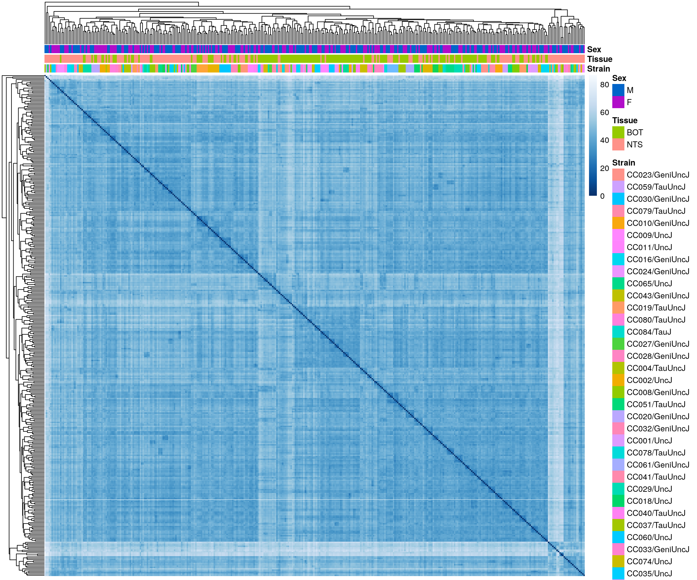
#heatmap on correlation matrix
rld_cor <- cor(assay(rld))
pheatmap(rld_cor,
annotation_col = df,
clustering_distance_rows = "correlation",
clustering_distance_cols = "correlation",
show_rownames = F, show_colnames = F,
annotation_colors = list(Tissue = c(BOT = "#96ca00",
NTS = "#ff9289"),
Sex = c("M" = "#0064C9",
"F" ="#B10DC9")),
border_color = NA)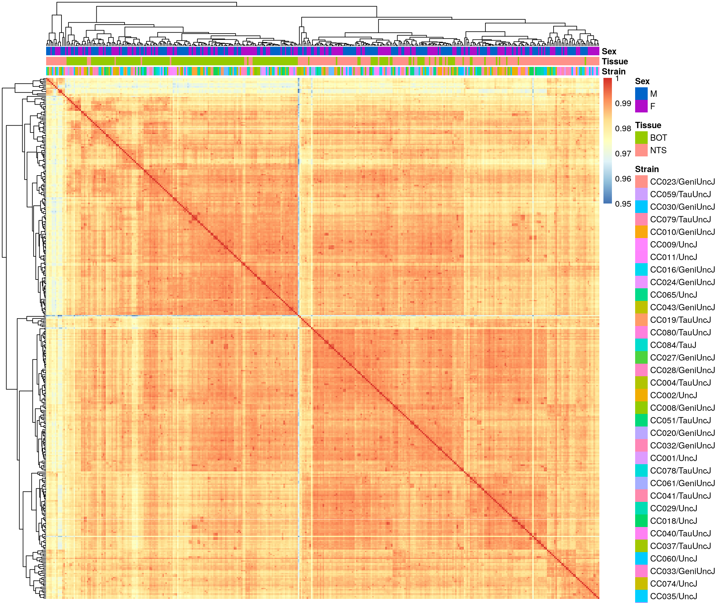
#PCA plot
#Another way to visualize sample-to-sample distances is a principal components analysis (PCA).
Batch <- plotPCA(rld, intgroup = c("Sex", "Tissue"), returnData = TRUE) %>%
dplyr::mutate(PCA_Batch = if_else(PC2 > -5, "Batch1", "Batch2"))
pca.plot <- plotPCA(rld, intgroup = c("Sex", "Tissue"), returnData = FALSE)
pca.plot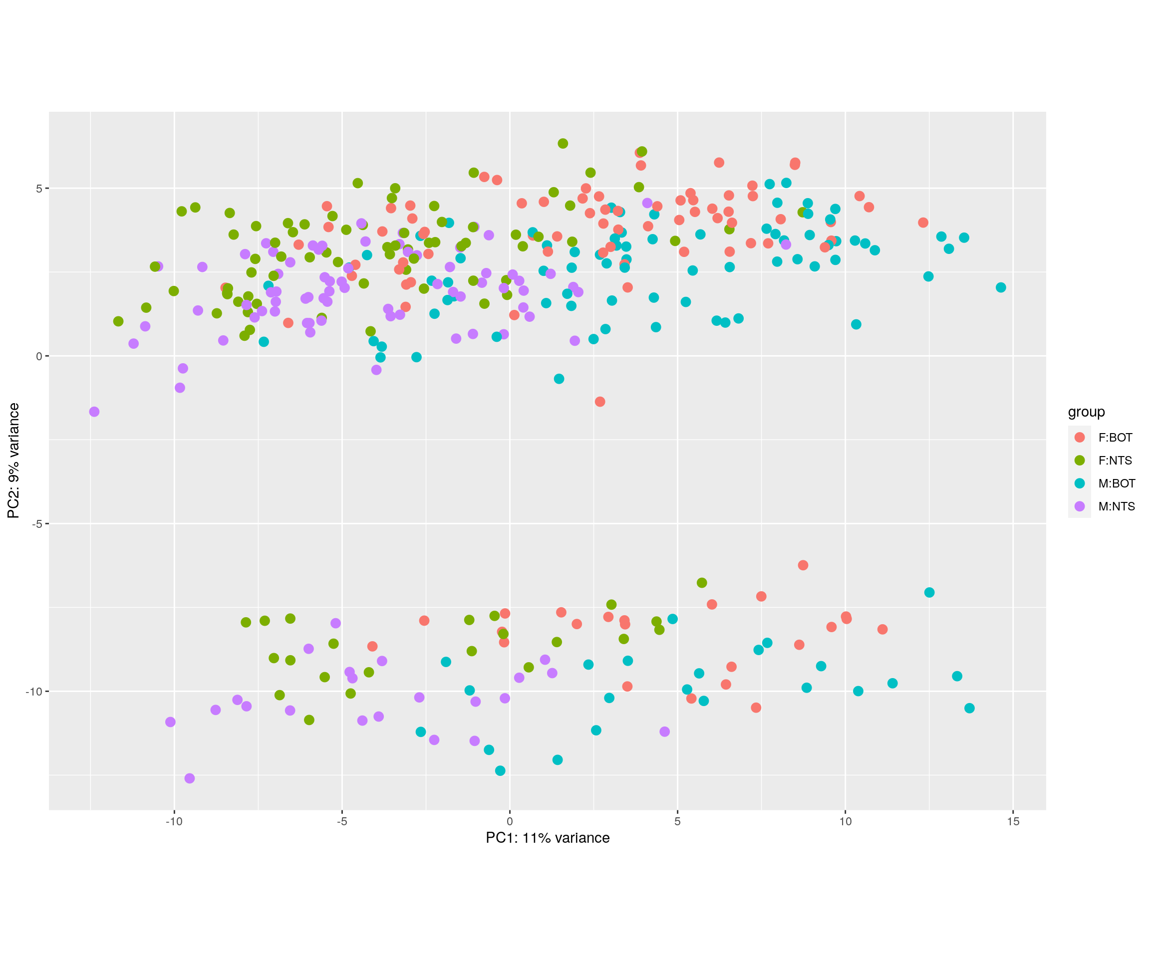
# calculate the variance for each gene
rv <- rowVars(assay(rld))
# Top n genes by variance to keep.
ntop <- 500
# select the ntop genes by variance
select <- order(rv, decreasing=TRUE)[seq_len(min(ntop, length(rv)))]
# perform a PCA on the data in assay(x) for the selected genes
pca <- prcomp(t(assay(rld)[select,]))
# Loadings for the first two PCs.
loadings <- pca$rotation[, seq_len(2)]
loadings <- as.data.frame(loadings) %>%
dplyr::arrange(desc(PC2)) %>%
tibble::rownames_to_column(var = "ENSEMBL") %>%
dplyr::left_join(genes) %>%
dplyr::slice(1:100)Joining, by = "ENSEMBL"#top100 genes driving PC2
DT::datatable(loadings,
filter = list(position = 'top', clear = FALSE),
extensions = 'Buttons',
options = list(dom = 'Blfrtip',
buttons = c('csv', 'excel'),
lengthMenu = list(c(10,25,50,-1),
c(10,25,50,"All")),
pageLength = 40,
scrollY = "300px",
scrollX = "40px"),
caption = htmltools::tags$caption(style = 'caption-side: top; text-align: left; color:black; font-size:200% ;','Top 100 genes driving PC2'))#sample_all_infor
sample_all_infor <- design.matrix %>%
dplyr::left_join(Batch[, c(3,6,7)]) %>%
dplyr::left_join(log)Joining, by = "name"Joining, by = "sampleid"#display sample_all_infor
DT::datatable(sample_all_infor,
filter = list(position = 'top', clear = FALSE),
extensions = 'Buttons',
options = list(dom = 'Blfrtip',
buttons = c('csv', 'excel'),
lengthMenu = list(c(10,25,50,-1),
c(10,25,50,"All")),
pageLength = 40,
scrollY = "300px",
scrollX = "40px"),
caption = htmltools::tags$caption(style = 'caption-side: top; text-align: left; color:black; font-size:200% ;','Sample all infor'))Differential expression analysis without interaction term
design(ddsMat)~Strain + Tissue + Sex#Running the differential expression pipeline
#res <- DESeq(ddsMat)
#save(res, file = "data/BOT_NTS_rnaseq_results/res_no_interaction.RData")
load("data/BOT_NTS_rnaseq_results/res_no_interaction.RData")
resultsNames(res) [1] "Intercept"
[2] "Strain_CC059.TauUncJ_vs_CC023.GeniUncJ"
[3] "Strain_CC030.GeniUncJ_vs_CC023.GeniUncJ"
[4] "Strain_CC079.TauUncJ_vs_CC023.GeniUncJ"
[5] "Strain_CC010.GeniUncJ_vs_CC023.GeniUncJ"
[6] "Strain_CC009.UncJ_vs_CC023.GeniUncJ"
[7] "Strain_CC011.UncJ_vs_CC023.GeniUncJ"
[8] "Strain_CC016.GeniUncJ_vs_CC023.GeniUncJ"
[9] "Strain_CC024.GeniUncJ_vs_CC023.GeniUncJ"
[10] "Strain_CC065.UncJ_vs_CC023.GeniUncJ"
[11] "Strain_CC043.GeniUncJ_vs_CC023.GeniUncJ"
[12] "Strain_CC019.TauUncJ_vs_CC023.GeniUncJ"
[13] "Strain_CC080.TauUncJ_vs_CC023.GeniUncJ"
[14] "Strain_CC084.TauJ_vs_CC023.GeniUncJ"
[15] "Strain_CC027.GeniUncJ_vs_CC023.GeniUncJ"
[16] "Strain_CC028.GeniUncJ_vs_CC023.GeniUncJ"
[17] "Strain_CC004.TauUncJ_vs_CC023.GeniUncJ"
[18] "Strain_CC002.UncJ_vs_CC023.GeniUncJ"
[19] "Strain_CC008.GeniUncJ_vs_CC023.GeniUncJ"
[20] "Strain_CC051.TauUncJ_vs_CC023.GeniUncJ"
[21] "Strain_CC020.GeniUncJ_vs_CC023.GeniUncJ"
[22] "Strain_CC032.GeniUncJ_vs_CC023.GeniUncJ"
[23] "Strain_CC001.UncJ_vs_CC023.GeniUncJ"
[24] "Strain_CC078.TauUncJ_vs_CC023.GeniUncJ"
[25] "Strain_CC061.GeniUncJ_vs_CC023.GeniUncJ"
[26] "Strain_CC041.TauUncJ_vs_CC023.GeniUncJ"
[27] "Strain_CC029.UncJ_vs_CC023.GeniUncJ"
[28] "Strain_CC018.UncJ_vs_CC023.GeniUncJ"
[29] "Strain_CC040.TauUncJ_vs_CC023.GeniUncJ"
[30] "Strain_CC037.TauUncJ_vs_CC023.GeniUncJ"
[31] "Strain_CC060.UncJ_vs_CC023.GeniUncJ"
[32] "Strain_CC033.GeniUncJ_vs_CC023.GeniUncJ"
[33] "Strain_CC074.UncJ_vs_CC023.GeniUncJ"
[34] "Strain_CC035.UncJ_vs_CC023.GeniUncJ"
[35] "Strain_CC058.UncJ_vs_CC023.GeniUncJ"
[36] "Strain_CC044.UncJ_vs_CC023.GeniUncJ"
[37] "Strain_CC015.UncJ_vs_CC023.GeniUncJ"
[38] "Strain_CC036.UncJ_vs_CC023.GeniUncJ"
[39] "Strain_CC012.GeniUncJ_vs_CC023.GeniUncJ"
[40] "Strain_CC013.GeniUncJ_vs_CC023.GeniUncJ"
[41] "Strain_CC026.GeniUncJ_vs_CC023.GeniUncJ"
[42] "Strain_CC083.UncJ_vs_CC023.GeniUncJ"
[43] "Strain_CC003.UncJ_vs_CC023.GeniUncJ"
[44] "Strain_CC017.UncJ_vs_CC023.GeniUncJ"
[45] "Strain_CC025.GeniUncJ_vs_CC023.GeniUncJ"
[46] "Strain_CC057.UncJ_vs_CC023.GeniUncJ"
[47] "Strain_CC005.TauUncJ_vs_CC023.GeniUncJ"
[48] "Strain_CC007.UncJ_vs_CC023.GeniUncJ"
[49] "Strain_CC068.TauUncJ_vs_CC023.GeniUncJ"
[50] "Strain_CC045.GeniUncJ_vs_CC023.GeniUncJ"
[51] "Strain_CC075.UncJ_vs_CC023.GeniUncJ"
[52] "Tissue_NTS_vs_BOT"
[53] "Sex_M_vs_F" #comparison for tissue------
#Building the results table
res.tab.tissue <- results(res, name = "Tissue_NTS_vs_BOT", alpha = 0.05)
res.tab.tissuelog2 fold change (MLE): Tissue NTS vs BOT
Wald test p-value: Tissue NTS vs BOT
DataFrame with 21651 rows and 6 columns
baseMean log2FoldChange lfcSE stat pvalue
<numeric> <numeric> <numeric> <numeric> <numeric>
ENSMUSG00000000001 1033.16866 -0.0792682 0.0139043 -5.70097 1.19127e-08
ENSMUSG00000000028 39.48781 -0.1474917 0.0347286 -4.24699 2.16665e-05
ENSMUSG00000000031 13.20458 -0.2441495 0.1369326 -1.78299 7.45878e-02
ENSMUSG00000000037 36.37264 0.3779521 0.0445468 8.48438 2.16868e-17
ENSMUSG00000000049 7.10111 -0.3899195 0.0918710 -4.24421 2.19369e-05
... ... ... ... ... ...
ENSMUSG00000118669 793.19118 0.0649345 0.0203550 3.190094 1.42226e-03
ENSMUSG00000118670 5.40400 1.0400916 0.1884189 5.520102 3.38803e-08
ENSMUSG00000118671 35.11590 0.5500835 0.0929598 5.917431 3.27008e-09
ENSMUSG00001074846 1.09017 0.1798469 0.2482523 0.724452 4.68788e-01
ENSMUSG00002076083 893.97259 -0.0235649 0.0144979 -1.625407 1.04076e-01
padj
<numeric>
ENSMUSG00000000001 4.17534e-08
ENSMUSG00000000028 5.36840e-05
ENSMUSG00000000031 1.06941e-01
ENSMUSG00000000037 1.65591e-16
ENSMUSG00000000049 5.43353e-05
... ...
ENSMUSG00000118669 2.77227e-03
ENSMUSG00000118670 1.13377e-07
ENSMUSG00000118671 1.21265e-08
ENSMUSG00001074846 5.37803e-01
ENSMUSG00002076083 1.43817e-01summary(res.tab.tissue)
out of 21651 with nonzero total read count
adjusted p-value < 0.05
LFC > 0 (up) : 7580, 35%
LFC < 0 (down) : 6425, 30%
outliers [1] : 50, 0.23%
low counts [2] : 0, 0%
(mean count < 0)
[1] see 'cooksCutoff' argument of ?results
[2] see 'independentFiltering' argument of ?resultstable(res.tab.tissue$padj < 0.05)
FALSE TRUE
7596 14005 #We subset the results table to these genes and then sort it by the log2 fold change estimate to get the significant genes with the strongest down-regulation:
resSig.tissue <- subset(res.tab.tissue, padj < 0.05)
head(resSig.tissue[order(resSig.tissue$log2FoldChange), ])log2 fold change (MLE): Tissue NTS vs BOT
Wald test p-value: Tissue NTS vs BOT
DataFrame with 6 rows and 6 columns
baseMean log2FoldChange lfcSE stat pvalue
<numeric> <numeric> <numeric> <numeric> <numeric>
ENSMUSG00000017311 25.40136 -5.96582 0.309039 -19.30443 4.92997e-83
ENSMUSG00000005892 226.18937 -3.52104 0.216531 -16.26111 1.86326e-59
ENSMUSG00000053706 8.81689 -3.45802 0.488044 -7.08545 1.38591e-12
ENSMUSG00000067220 4.48264 -3.07749 0.560055 -5.49497 3.90778e-08
ENSMUSG00000020838 387.60082 -3.01105 0.232740 -12.93739 2.76878e-38
ENSMUSG00000020713 7.07753 -2.88929 0.502730 -5.74719 9.07390e-09
padj
<numeric>
ENSMUSG00000017311 5.91624e-80
ENSMUSG00000005892 3.79701e-57
ENSMUSG00000053706 7.02581e-12
ENSMUSG00000067220 1.29785e-07
ENSMUSG00000020838 1.11375e-36
ENSMUSG00000020713 3.21267e-08# with the strongest up-regulation:
head(resSig.tissue[order(resSig.tissue$log2FoldChange, decreasing = TRUE), ])log2 fold change (MLE): Tissue NTS vs BOT
Wald test p-value: Tissue NTS vs BOT
DataFrame with 6 rows and 6 columns
baseMean log2FoldChange lfcSE stat pvalue
<numeric> <numeric> <numeric> <numeric> <numeric>
ENSMUSG00000000394 12.93068 5.97558 0.675039 8.85221 8.58052e-19
ENSMUSG00000016458 2.24815 4.75478 0.937585 5.07130 3.95101e-07
ENSMUSG00000000690 52.60788 4.45144 0.417147 10.67115 1.38899e-26
ENSMUSG00000045232 98.46575 4.01304 0.408825 9.81603 9.60542e-23
ENSMUSG00000038721 9.41743 3.90721 0.484252 8.06856 7.11313e-16
ENSMUSG00000072845 4.04600 3.82237 0.617873 6.18634 6.15789e-10
padj
<numeric>
ENSMUSG00000000394 7.26854e-18
ENSMUSG00000016458 1.18191e-06
ENSMUSG00000000690 2.18208e-25
ENSMUSG00000045232 1.11612e-21
ENSMUSG00000038721 4.79111e-15
ENSMUSG00000072845 2.43620e-09#comparison for Sex------
#Building the results table
res.tab.sex <- results(res, name = "Sex_M_vs_F", alpha = 0.05)
res.tab.sexlog2 fold change (MLE): Sex M vs F
Wald test p-value: Sex M vs F
DataFrame with 21651 rows and 6 columns
baseMean log2FoldChange lfcSE stat pvalue
<numeric> <numeric> <numeric> <numeric> <numeric>
ENSMUSG00000000001 1033.16866 0.01392084 0.0141801 0.9817190 0.326238
ENSMUSG00000000028 39.48781 0.04466003 0.0354254 1.2606779 0.207425
ENSMUSG00000000031 13.20458 -0.02195904 0.1397346 -0.1571482 0.875128
ENSMUSG00000000037 36.37264 -0.10667388 0.0455009 -2.3444346 0.019056
ENSMUSG00000000049 7.10111 -0.00513409 0.0933996 -0.0549691 0.956163
... ... ... ... ... ...
ENSMUSG00000118669 793.19118 -0.0209681 0.0207593 -1.0100558 0.3124686
ENSMUSG00000118670 5.40400 -0.2065203 0.1921793 -1.0746232 0.2825435
ENSMUSG00000118671 35.11590 0.1755270 0.0948575 1.8504291 0.0642517
ENSMUSG00001074846 1.09017 0.0200659 0.2531294 0.0792713 0.9368168
ENSMUSG00002076083 893.97259 0.0031614 0.0147863 0.2138064 0.8306980
padj
<numeric>
ENSMUSG00000000001 0.828149
ENSMUSG00000000028 0.742921
ENSMUSG00000000031 0.980655
ENSMUSG00000000037 0.362627
ENSMUSG00000000049 0.994334
... ...
ENSMUSG00000118669 0.817234
ENSMUSG00000118670 0.802720
ENSMUSG00000118671 0.536900
ENSMUSG00001074846 NA
ENSMUSG00002076083 0.974957summary(res.tab.sex)
out of 21651 with nonzero total read count
adjusted p-value < 0.05
LFC > 0 (up) : 70, 0.32%
LFC < 0 (down) : 74, 0.34%
outliers [1] : 50, 0.23%
low counts [2] : 1677, 7.7%
(mean count < 3)
[1] see 'cooksCutoff' argument of ?results
[2] see 'independentFiltering' argument of ?resultstable(res.tab.sex$padj < 0.05)
FALSE TRUE
19780 144 #We subset the results table to these genes and then sort it by the log2 fold change estimate to get the significant genes with the strongest down-regulation:
resSig.sex <- subset(res.tab.sex, padj < 0.05)
head(resSig.sex[order(resSig.sex$log2FoldChange), ])log2 fold change (MLE): Sex M vs F
Wald test p-value: Sex M vs F
DataFrame with 6 rows and 6 columns
baseMean log2FoldChange lfcSE stat pvalue
<numeric> <numeric> <numeric> <numeric> <numeric>
ENSMUSG00000021342 8.26656 -5.975428 0.5010197 -11.92653 8.60858e-33
ENSMUSG00000085715 60.25368 -4.314587 0.1487615 -29.00339 5.96308e-185
ENSMUSG00000048173 5.48188 -2.618359 0.3421339 -7.65303 1.96305e-14
ENSMUSG00000049123 5.40062 -0.603931 0.1666143 -3.62473 2.89267e-04
ENSMUSG00000035150 6131.08143 -0.544192 0.0144834 -37.57358 0.00000e+00
ENSMUSG00000037369 1158.33575 -0.531282 0.0188680 -28.15783 1.92159e-174
padj
<numeric>
ENSMUSG00000021342 1.14345e-29
ENSMUSG00000085715 1.69726e-181
ENSMUSG00000048173 2.17288e-11
ENSMUSG00000049123 4.27156e-02
ENSMUSG00000035150 0.00000e+00
ENSMUSG00000037369 4.78572e-171# with the strongest up-regulation:
head(resSig.sex[order(resSig.sex$log2FoldChange, decreasing = TRUE), ])log2 fold change (MLE): Sex M vs F
Wald test p-value: Sex M vs F
DataFrame with 6 rows and 6 columns
baseMean log2FoldChange lfcSE stat pvalue
<numeric> <numeric> <numeric> <numeric> <numeric>
ENSMUSG00000069044 5.6855 16.09354 2.959846 5.43729 5.40969e-08
ENSMUSG00000069045 1120.7806 14.69784 0.314964 46.66521 0.00000e+00
ENSMUSG00000069049 423.0885 13.10033 0.300101 43.65312 0.00000e+00
ENSMUSG00000068457 523.1966 11.70615 0.277993 42.10949 0.00000e+00
ENSMUSG00000056673 614.5115 9.99808 0.236786 42.22415 0.00000e+00
ENSMUSG00000099876 17.3208 6.88914 0.219910 31.32708 1.99678e-215
padj
<numeric>
ENSMUSG00000069044 3.71664e-05
ENSMUSG00000069045 0.00000e+00
ENSMUSG00000069049 0.00000e+00
ENSMUSG00000068457 0.00000e+00
ENSMUSG00000056673 0.00000e+00
ENSMUSG00000099876 6.63063e-212Visualization
#Visualization for tissue result------
#Volcano plot
## Obtain logical vector regarding whether padj values are less than 0.05
threshold_OE <- (res.tab.tissue$padj < 0.05 & abs(res.tab.tissue$log2FoldChange) >= 1)
## Determine the number of TRUE values
length(which(threshold_OE))[1] 498## Add logical vector as a column (threshold) to the res.tab.tissue
res.tab.tissue$threshold <- threshold_OE
## Sort by ordered padj
res.tab.tissue_ordered <- res.tab.tissue %>%
data.frame() %>%
rownames_to_column(var="ENSEMBL") %>%
arrange(padj) %>%
mutate(genelabels = "") %>%
as_tibble() %>%
left_join(genes)Joining, by = "ENSEMBL"## Create a column to indicate which genes to label
res.tab.tissue_ordered$genelabels[1:10] <- res.tab.tissue_ordered$SYMBOL[1:10]
#display res.tab.tissue_ordered
DT::datatable(res.tab.tissue_ordered[res.tab.tissue_ordered$padj < 0.05,],
filter = list(position = 'top', clear = FALSE),
extensions = 'Buttons',
options = list(dom = 'Blfrtip',
buttons = c('csv', 'excel'),
lengthMenu = list(c(10,25,50,-1),
c(10,25,50,"All")),
pageLength = 40,
scrollY = "300px",
scrollX = "40px"),
caption = htmltools::tags$caption(style = 'caption-side: top; text-align: left; color:black; font-size:200% ;','DEG analysis tissue results (fdr < 0.05)'))Warning in instance$preRenderHook(instance): It seems your data is too big
for client-side DataTables. You may consider server-side processing: https://
rstudio.github.io/DT/server.html#Volcano plot
volcano.plot.tissue <- ggplot(res.tab.tissue_ordered) +
geom_point(aes(x = log2FoldChange, y = -log10(padj), colour = threshold)) +
scale_color_manual(values=c("blue", "red")) +
geom_text_repel(aes(x = log2FoldChange, y = -log10(padj),
label = genelabels,
size = 3.5)) +
ggtitle("DEG for Tissue NTS vs BOT") +
xlab("log2 fold change") +
ylab("-log10 adjusted p-value") +
theme(legend.position = "none",
plot.title = element_text(size = rel(1.5), hjust = 0.5),
axis.title = element_text(size = rel(1.25)))
print(volcano.plot.tissue)Warning: Removed 50 rows containing missing values (geom_point).Warning: Removed 50 rows containing missing values (geom_text_repel).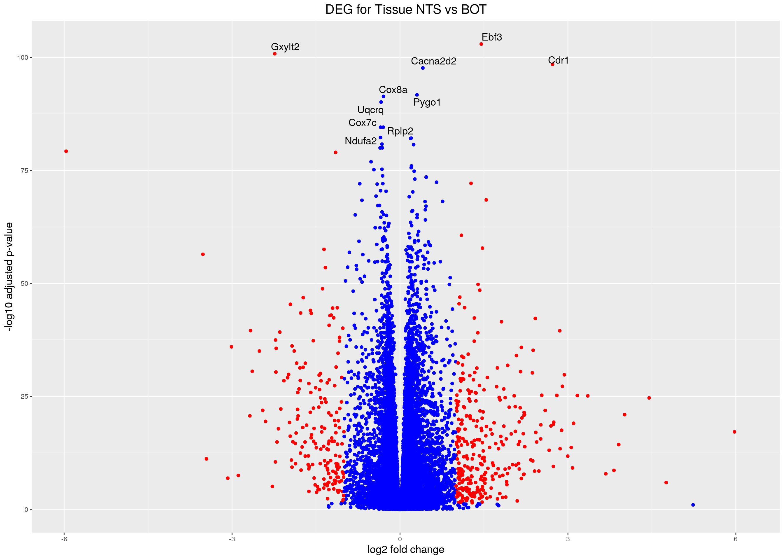
#heatmap
# Extract normalized expression for significant genes fdr < 0.05 & abs(log2FoldChange) >= 1)
normalized_counts_sig.tissue <- normalized_counts %>%
filter(gene %in% rownames(subset(resSig.tissue, padj < 0.05 & abs(log2FoldChange) >= 1)))
### Set a color palette
heat_colors <- brewer.pal(6, "YlOrRd")
#annotation
df <- as.data.frame(colData(ddsMat)[,c("Strain","Tissue", "Sex")])
### Run pheatmap using the metadata data frame for the annotation
dat = as.matrix(normalized_counts_sig.tissue[,-1])
colnames(dat) = rownames(df)
pheatmap(dat,
color = heat_colors,
cluster_rows = T,
show_rownames = F,
annotation_col = df,
annotation_colors = list(Tissue = c(BOT = "#96ca00",
NTS = "#ff9289"),
Sex = c("M" = "#0064C9",
"F" ="#B10DC9")),
border_color = NA,
fontsize = 10,
scale = "row",
fontsize_row = 10,
height = 20,
main = "Heatmap of the top DEGs in Tissue NTS vs Bot (fdr < 0.05 & abs(log2FoldChange) >= 1)")
#Visualization for Sex result------
#Volcano plot
## Obtain logical vector regarding whether padj values are less than 0.05
threshold_OE <- (res.tab.sex$padj < 0.05 & abs(res.tab.sex$log2FoldChange) >= 1)
## Determine the number of TRUE values
length(which(threshold_OE))[1] 10## Add logical vector as a column (threshold) to the res.tab.sex
res.tab.sex$threshold <- threshold_OE
## Sort by ordered padj
res.tab.sex_ordered <- res.tab.sex %>%
data.frame() %>%
rownames_to_column(var="ENSEMBL") %>%
arrange(padj) %>%
mutate(genelabels = "") %>%
as_tibble() %>%
left_join(genes)Joining, by = "ENSEMBL"## Create a column to indicate which genes to label
res.tab.sex_ordered$genelabels[1:10] <- res.tab.sex_ordered$SYMBOL[1:10]
#display res.tab.sex_ordered
DT::datatable(res.tab.sex_ordered[res.tab.sex_ordered$padj < 0.05,],
filter = list(position = 'top', clear = FALSE),
extensions = 'Buttons',
options = list(dom = 'Blfrtip',
buttons = c('csv', 'excel'),
lengthMenu = list(c(10,25,50,-1),
c(10,25,50,"All")),
pageLength = 40,
scrollY = "300px",
scrollX = "40px"),
caption = htmltools::tags$caption(style = 'caption-side: top; text-align: left; color:black; font-size:200% ;','DEG analysis sex results (fdr < 0.05)'))#Volcano plot
volcano.plot.sex <- ggplot(res.tab.sex_ordered) +
geom_point(aes(x = log2FoldChange, y = -log10(padj), colour = threshold)) +
scale_color_manual(values=c("blue", "red")) +
geom_text_repel(aes(x = log2FoldChange, y = -log10(padj),
label = genelabels,
size = 3.5)) +
ggtitle("DEG for sex Male vs Female") +
xlab("log2 fold change") +
ylab("-log10 adjusted p-value") +
theme(legend.position = "none",
plot.title = element_text(size = rel(1.5), hjust = 0.5),
axis.title = element_text(size = rel(1.25)))
#print(volcano.plot.sex)
#heatmap
# Extract normalized expression for significant genes fdr < 0.05 & abs(log2FoldChange) >= 1)
normalized_counts_sig.sex <- normalized_counts %>%
filter(gene %in% rownames(subset(resSig.sex, padj < 0.05 & abs(log2FoldChange) >= 1)))
### Set a color palette
heat_colors <- brewer.pal(6, "YlOrRd")
#annotation
df <- as.data.frame(colData(ddsMat)[,c("Strain","Tissue", "Sex")])
### Run pheatmap using the metadata data frame for the annotation
dat = as.matrix(normalized_counts_sig.sex[,-1])
colnames(dat) = rownames(df)
pheatmap(dat,
color = heat_colors,
cluster_rows = T,
show_rownames = F,
annotation_col = df,
annotation_colors = list(Tissue = c(BOT = "#96ca00",
NTS = "#ff9289"),
Sex = c("M" = "#0064C9",
"F" ="#B10DC9")),
border_color = NA,
fontsize = 10,
scale = "row",
fontsize_row = 10,
height = 20,
main = "Heatmap of the top DEGs in Sex Male vs Femal(fdr < 0.05 & abs(log2FoldChange) >= 1)")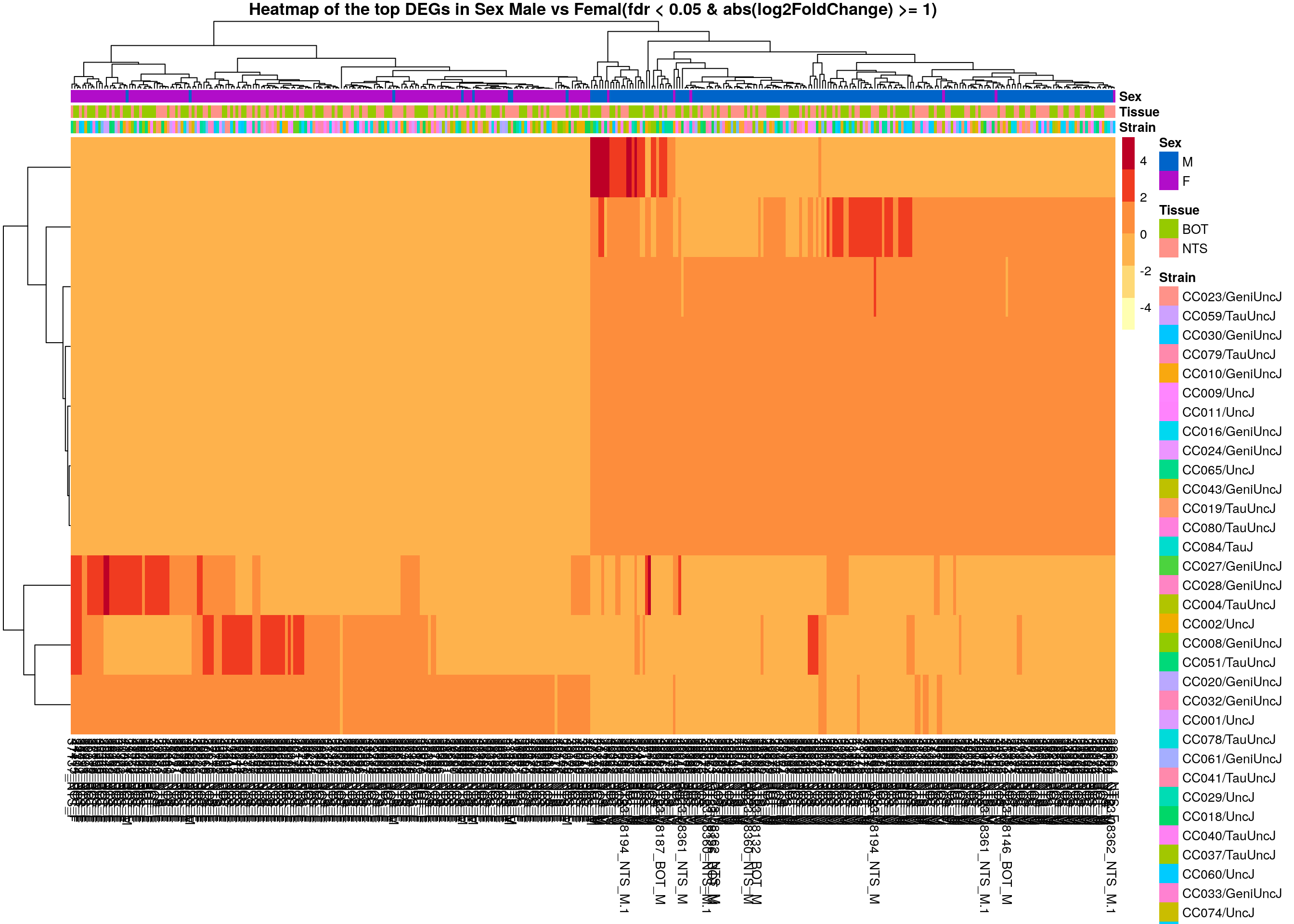
#heatmap on both sex and tissue top DEGs-----
normalized_counts_sig.sex.tissue <- normalized_counts %>%
filter(gene %in% unique(rownames(subset(resSig.tissue, padj < 0.05 & abs(log2FoldChange) >= 1)),
rownames(subset(resSig.sex, padj < 0.05 & abs(log2FoldChange) >= 1))))
### Set a color palette
heat_colors <- brewer.pal(6, "YlOrRd")
#annotation
df <- as.data.frame(colData(ddsMat)[,c("Strain","Tissue", "Sex")])
### Run pheatmap using the metadata data frame for the annotation
dat = as.matrix(normalized_counts_sig.sex.tissue[,-1])
colnames(dat) = rownames(df)
pheatmap(dat,
color = heat_colors,
cluster_rows = T,
show_rownames = F,
annotation_col = df,
annotation_colors = list(Tissue = c(BOT = "#96ca00",
NTS = "#ff9289"),
Sex = c("M" = "#0064C9",
"F" ="#B10DC9")),
border_color = NA,
fontsize = 10,
scale = "row",
fontsize_row = 10,
height = 20,
main = "Heatmap of the top DEGs in Both Sex and Tissue (fdr < 0.05 & abs(log2FoldChange) >= 1)")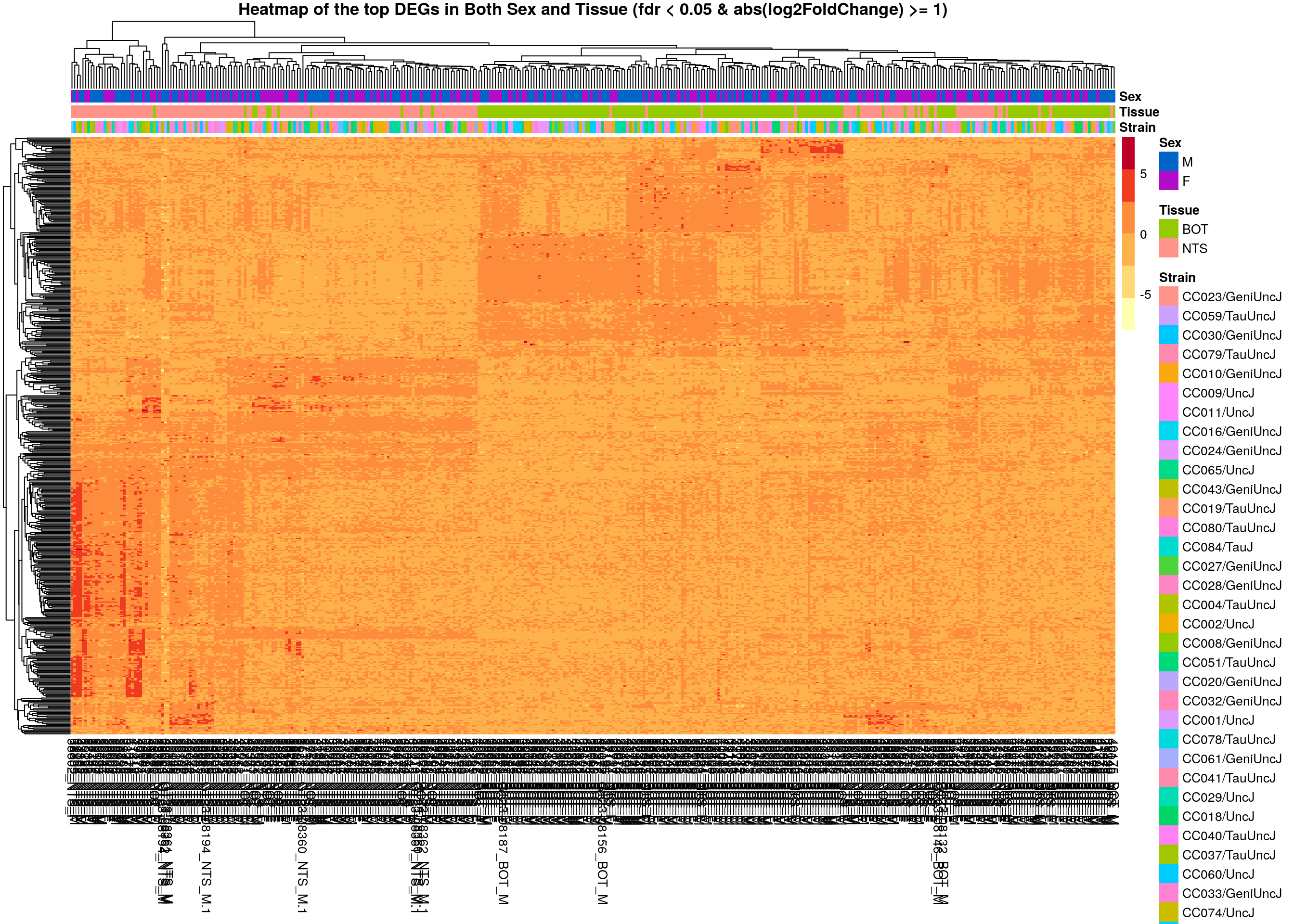
#logFC heatmap on both sex and tissue top DEGs-----
restop.tab.sex.tissue <- full_join(res.tab.sex_ordered,
res.tab.tissue_ordered,
by = c("ENSEMBL", "SYMBOL")) %>%
filter((ENSEMBL %in% res.tab.sex_ordered$ENSEMBL[1:30]) | (ENSEMBL %in% res.tab.tissue_ordered$ENSEMBL[1:30]))
restop.tab.sex.tissue.mat <- as.matrix(restop.tab.sex.tissue[, c("log2FoldChange.x", "log2FoldChange.y")])
rownames(restop.tab.sex.tissue.mat) <-
ifelse(is.na(restop.tab.sex.tissue$SYMBOL),
restop.tab.sex.tissue$ENSEMBL,
paste0(restop.tab.sex.tissue$SYMBOL,":", restop.tab.sex.tissue$ENSEMBL))
colnames(restop.tab.sex.tissue.mat) <- c("sex", "tissue")
#heatmap
### Run pheatmap using the metadata data frame for the annotation
pheatmap(restop.tab.sex.tissue.mat,
color = colorpanel(1000, "blue", "white", "red"),
cluster_rows = T,
show_rownames = T,
border_color = NA,
fontsize = 10,
fontsize_row = 8,
height = 25,
main = "Heatmap of log2FoldChange for the top 30 DEGs in Sex or Tissue")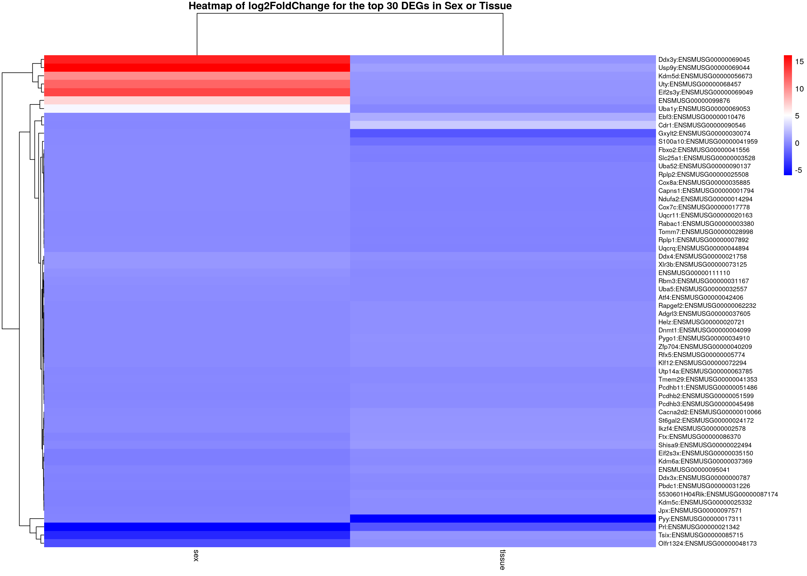
Enrichment
#enrichment analysis
dbs <- c("WikiPathways_2019_Mouse",
"GO_Biological_Process_2021",
"GO_Cellular_Component_2021",
"GO_Molecular_Function_2021",
"KEGG_2019_Mouse",
"Mouse_Gene_Atlas",
"MGI_Mammalian_Phenotype_Level_4_2019")
#tissue results------
resSig.tissue.tab <- resSig.tissue %>%
data.frame() %>%
rownames_to_column(var="ENSEMBL") %>%
as_tibble() %>%
left_join(genes)Joining, by = "ENSEMBL"#up-regulated tissue genes---------------------------
up.genes <- resSig.tissue.tab %>%
filter(log2FoldChange > 0) %>%
pull(SYMBOL)
#up-regulated genes enrichment
up.genes.enriched <- enrichr(as.character(na.omit(up.genes)), dbs)Uploading data to Enrichr... Done.
Querying WikiPathways_2019_Mouse... Done.
Querying GO_Biological_Process_2021... Done.
Querying GO_Cellular_Component_2021... Done.
Querying GO_Molecular_Function_2021... Done.
Querying KEGG_2019_Mouse... Done.
Querying Mouse_Gene_Atlas... Done.
Querying MGI_Mammalian_Phenotype_Level_4_2019... Done.
Parsing results... Done.for (j in 1:length(up.genes.enriched)){
up.genes.enriched[[j]] <- cbind(data.frame(Library = names(up.genes.enriched)[j]),up.genes.enriched[[j]])
}
up.genes.enriched <- do.call(rbind.data.frame, up.genes.enriched) %>%
filter(Adjusted.P.value <= 0.05) %>%
mutate(logpvalue = -log10(P.value)) %>%
arrange(desc(logpvalue))
#display up.genes.enriched
DT::datatable(up.genes.enriched,filter = list(position = 'top', clear = FALSE),
extensions = 'Buttons',
options = list(dom = 'Blfrtip',
buttons = c('csv', 'excel'),
lengthMenu = list(c(10,25,50,-1),
c(10,25,50,"All")),
pageLength = 40,
scrollY = "300px",
scrollX = "40px")
)#barpot
up.genes.enriched.plot <- up.genes.enriched %>%
filter(Adjusted.P.value <= 0.001) %>%
mutate(Term = fct_reorder(Term, -logpvalue)) %>%
ggplot(data = ., aes(x = Term, y = logpvalue, fill = Library, label = Overlap)) +
geom_bar(stat = "identity") +
geom_text(position = position_dodge(width = 0.9),
hjust = 0) +
theme_bw() +
ylab("-log(p.value)") +
xlab("") +
ggtitle("Enrichment of up-regulated tissue genes \n(Adjusted.P.value <= 0.001)") +
theme(plot.background = element_blank() ,
panel.border = element_blank(),
panel.background = element_blank(),
#legend.position = "none",
plot.title = element_text(hjust = 0),
panel.grid.major = element_blank(),
panel.grid.minor = element_blank()) +
theme(axis.line = element_line(color = 'black')) +
theme(axis.title.x = element_text(size = 12, vjust=-0.5)) +
theme(axis.title.y = element_text(size = 12, vjust= 1.0)) +
theme(axis.text = element_text(size = 12)) +
theme(plot.title = element_text(size = 12)) +
coord_flip()
up.genes.enriched.plot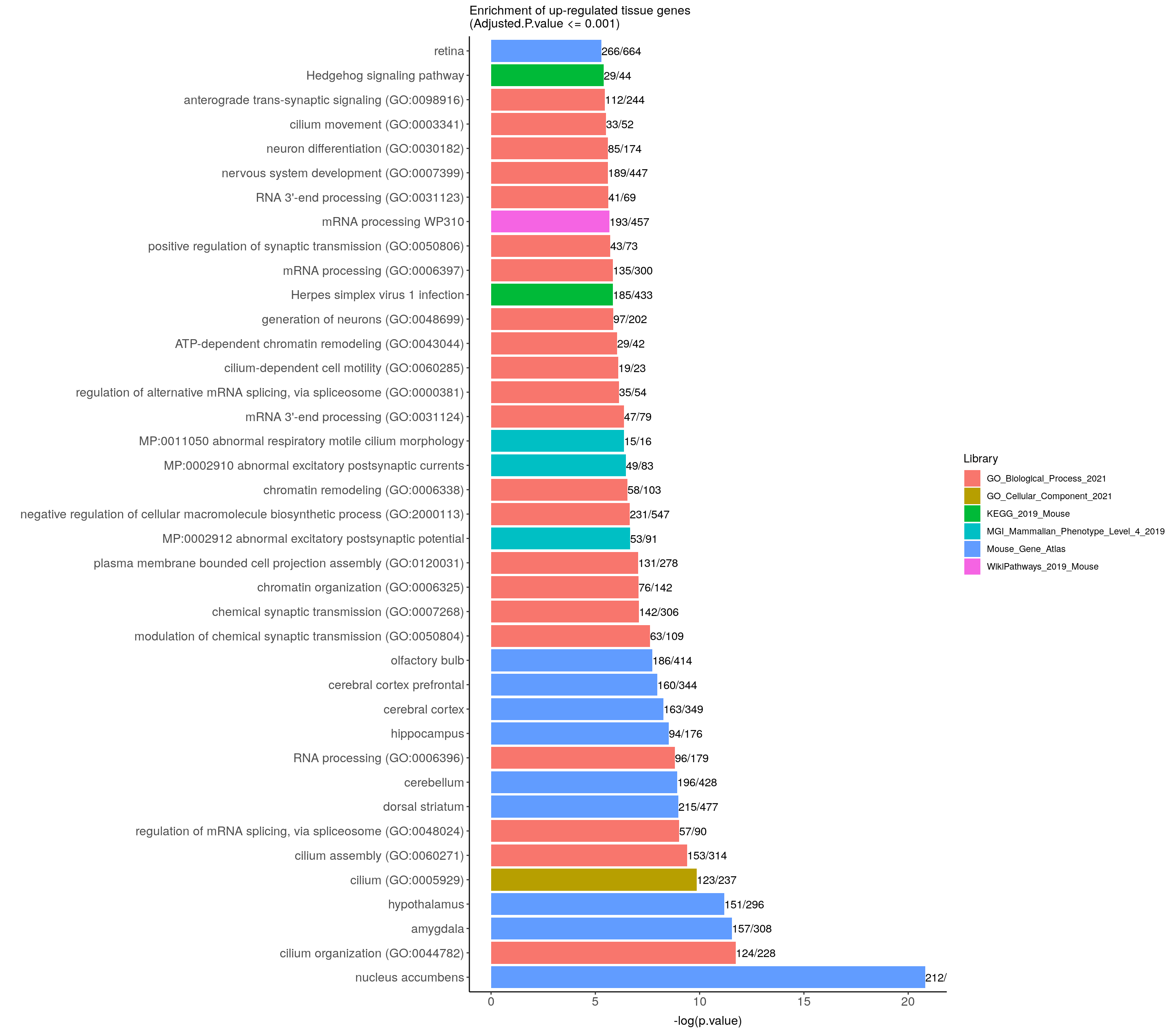
#down-regulated tissue genes---------------------------
down.genes <- resSig.tissue.tab %>%
filter(log2FoldChange < 0) %>%
pull(SYMBOL)
#down-regulated genes enrichment
down.genes.enriched <- enrichr(as.character(na.omit(down.genes)), dbs)Uploading data to Enrichr... Done.
Querying WikiPathways_2019_Mouse... Done.
Querying GO_Biological_Process_2021... Done.
Querying GO_Cellular_Component_2021... Done.
Querying GO_Molecular_Function_2021... Done.
Querying KEGG_2019_Mouse... Done.
Querying Mouse_Gene_Atlas... Done.
Querying MGI_Mammalian_Phenotype_Level_4_2019... Done.
Parsing results... Done.for (j in 1:length(down.genes.enriched)){
down.genes.enriched[[j]] <- cbind(data.frame(Library = names(down.genes.enriched)[j]),down.genes.enriched[[j]])
}
down.genes.enriched <- do.call(rbind.data.frame, down.genes.enriched) %>%
filter(Adjusted.P.value <= 0.05) %>%
mutate(logpvalue = -log10(P.value)) %>%
arrange(desc(logpvalue))
#display down.genes.enriched
DT::datatable(down.genes.enriched,
filter = list(position = 'top', clear = FALSE),
extensions = 'Buttons',
options = list(dom = 'Blfrtip',
buttons = c('csv', 'excel'),
lengthMenu = list(c(10,25,50,-1),
c(10,25,50,"All")),
pageLength = 40,
scrollY = "300px",
scrollX = "40px")
)#barpot
down.genes.enriched.plot <- down.genes.enriched %>%
filter(Adjusted.P.value <= 0.0000001) %>%
mutate(Term = fct_reorder(Term, -logpvalue)) %>%
ggplot(data = ., aes(x = Term, y = logpvalue, fill = Library, label = Overlap)) +
geom_bar(stat = "identity") +
geom_text(position = position_dodge(width = 0.9),
hjust = 0) +
theme_bw() +
ylab("-log(p.value)") +
xlab("") +
ggtitle("Enrichment of down-regulated tissue genes \n(Adjusted.P.value <= 0.0000001)") +
theme(plot.background = element_blank() ,
panel.border = element_blank(),
panel.background = element_blank(),
#legend.position = "none",
plot.title = element_text(hjust = 0),
panel.grid.major = element_blank(),
panel.grid.minor = element_blank()) +
theme(axis.line = element_line(color = 'black')) +
theme(axis.title.x = element_text(size = 12, vjust=-0.5)) +
theme(axis.title.y = element_text(size = 12, vjust= 1.0)) +
theme(axis.text = element_text(size = 12)) +
theme(plot.title = element_text(size = 12)) +
coord_flip()
down.genes.enriched.plot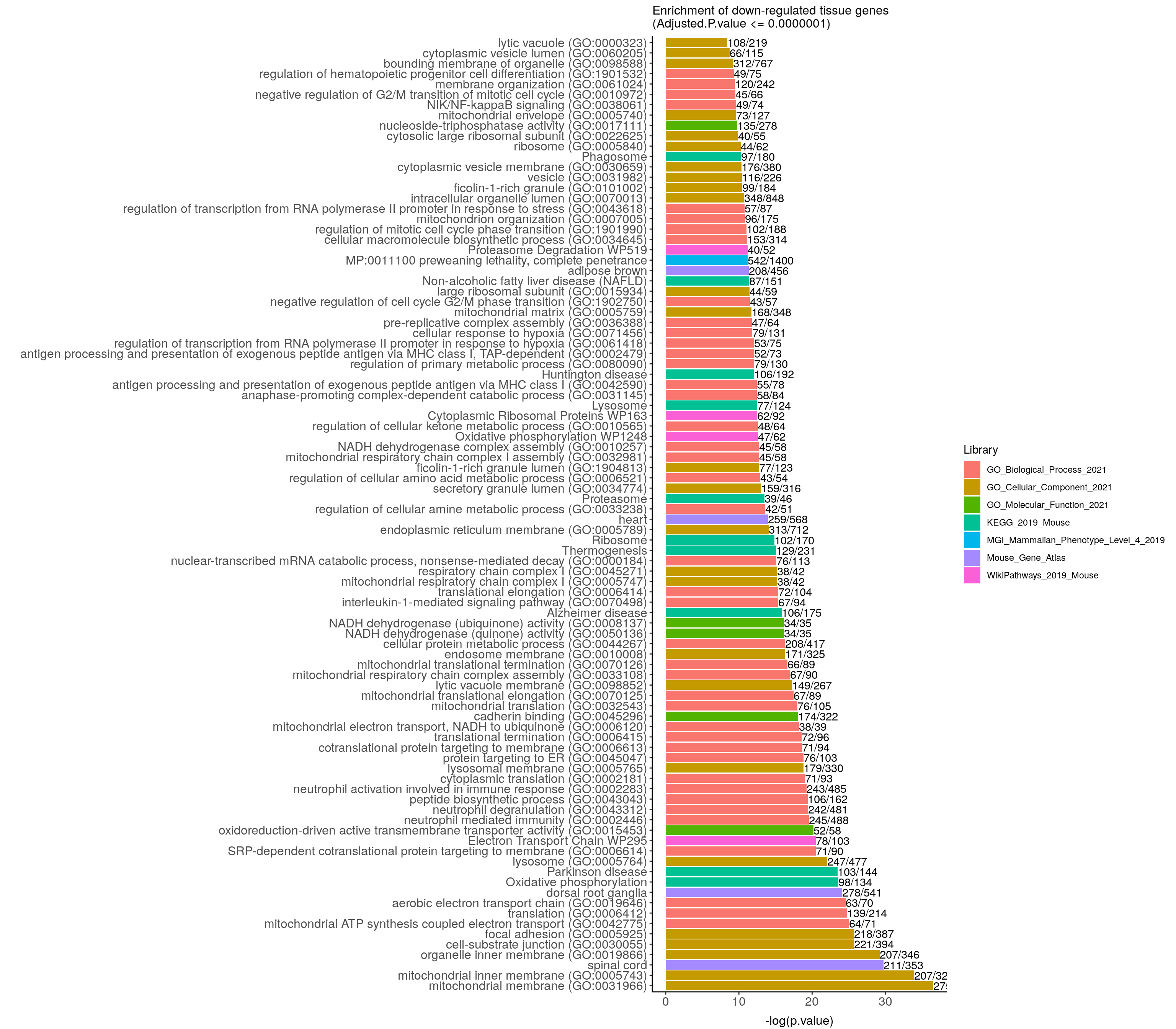
WGCNA for combined datasets
#Setting string not as factor
options(stringsAsFactors = FALSE)
#Enable multithread
enableWGCNAThreads(nThreads = 10)Allowing parallel execution with up to 10 working processes.#heatmap
make_module_heatmap <- function(module_name,
expression_mat = normalized_counts,
metadata_df = metadata,
gene_module_key_df = gene_module_key,
module_eigengenes_df = module_eigengenes) {
# Create a summary heatmap of a given module.
#
# Args:
# module_name: a character indicating what module should be plotted, e.g. "ME19"
# expression_mat: The full gene expression matrix. Default is `normalized_counts`.
# metadata_df: a data frame with refinebio_accession_code and time_point
# as columns. Default is `metadata`.
# gene_module_key: a data.frame indicating what genes are a part of what modules. Default is `gene_module_key`.
# module_eigengenes: a sample x eigengene data.frame with samples as row names. Default is `module_eigengenes`.
#
# Returns:
# A heatmap of expression matrix for a module's genes, with a barplot of the
# eigengene expression for that module.
# Set up the module eigengene with its Name
module_eigengene <- module_eigengenes_df %>%
dplyr::select(all_of(module_name)) %>%
tibble::rownames_to_column("Name")
# Set up column annotation from metadata
col_annot_df <- metadata_df %>%
tibble::rownames_to_column("Name") %>%
# Add on the eigengene expression by joining with sample IDs
dplyr::inner_join(module_eigengene, by = "Name") %>%
# Arrange by patient and time point
dplyr::arrange(Name, Strain) %>%
# Store sample
tibble::column_to_rownames("Name")
# Create the ComplexHeatmap column annotation object
col_annot <- ComplexHeatmap::HeatmapAnnotation(
# Supply treatment labels
Strain = col_annot_df$Strain,
#annotation_label = unique(col_annot_df$Strain),
#show_legend = FALSE,
# Add annotation barplot
module_eigengene = ComplexHeatmap::anno_barplot(dplyr::select(col_annot_df, module_name))
)
# Get a vector of the Ensembl gene IDs that correspond to this module
module_genes <- gene_module_key_df %>%
dplyr::filter(module == module_name) %>%
dplyr::pull(gene)
# Set up the gene expression data frame
mod_mat <- expression_mat %>%
t() %>%
as.data.frame() %>%
# Only keep genes from this module
dplyr::filter(rownames(.) %in% module_genes) %>%
# Order the samples to match col_annot_df
dplyr::select(rownames(col_annot_df)) %>%
# Data needs to be a matrix
as.matrix()
# Normalize the gene expression values
mod_mat <- mod_mat %>%
# Scale can work on matrices, but it does it by column so we will need to
# transpose first
t() %>%
scale() %>%
# And now we need to transpose back
t()
# Create a color function based on standardized scale
color_func <- circlize::colorRamp2(
c(-2, 0, 2),
c("#67a9cf", "#f7f7f7", "#ef8a62")
)
# Plot on a heatmap
heatmap <- ComplexHeatmap::Heatmap(mod_mat,
name = module_name,
# Supply color function
col = color_func,
# Supply column annotation
bottom_annotation = col_annot,
# We don't want to cluster samples
cluster_columns = FALSE,
# We don't need to show sample or gene labels
show_row_names = FALSE,
show_column_names = FALSE,
show_heatmap_legend = FALSE
)
lgd = ComplexHeatmap::Legend(labels = unique(col_annot_df$Strain),
legend_gp = gpar(fill = 1:length(unique(col_annot_df$Strain))),
title = "Strain",
row_gap = unit(40, "mm"),
ncol = 2, title_position = "topcenter")
# Return heatmap
return(heatmap)
#draw(heatmap, annotation_legend_list = lgd)
}
load("data/BOT_NTS_rnaseq_results/rld.RData")
expression = t(assay(rld))
#Determine parameters for WGCNA
sft <- pickSoftThreshold(expression,
dataIsExpr = TRUE,
corFnc = cor,
networkType = "signed"
) Power SFT.R.sq slope truncated.R.sq mean.k. median.k. max.k.
1 1 0.0904 24.30 0.970 10900.00 1.09e+04 11200.0
2 2 0.1140 -13.20 0.922 5570.00 5.55e+03 6080.0
3 3 0.3680 -13.40 0.895 2920.00 2.89e+03 3480.0
4 4 0.6080 -10.20 0.940 1560.00 1.53e+03 2090.0
5 5 0.7220 -7.53 0.970 850.00 8.24e+02 1310.0
6 6 0.7700 -5.93 0.977 474.00 4.51e+02 854.0
7 7 0.7990 -4.82 0.977 270.00 2.51e+02 579.0
8 8 0.8100 -4.04 0.968 158.00 1.42e+02 404.0
9 9 0.8310 -3.40 0.968 94.50 8.13e+01 289.0
10 10 0.8510 -2.93 0.969 58.10 4.73e+01 211.0
11 12 0.7950 -2.75 0.935 23.80 1.67e+01 132.0
12 14 0.8050 -2.60 0.962 10.90 6.22e+00 91.7
13 16 0.8380 -2.38 0.981 5.49 2.45e+00 67.8
14 18 0.8620 -2.22 0.988 3.03 1.01e+00 52.1
15 20 0.8930 -2.06 0.993 1.80 4.38e-01 41.2sft_df <- data.frame(sft$fitIndices) %>%
dplyr::mutate(model_fit = -sign(slope) * SFT.R.sq)
ggplot(sft_df, aes(x = Power, y = model_fit, label = Power)) +
# Plot the points
geom_point() +
# We'll put the Power labels slightly above the data points
geom_text(nudge_y = 0.1) +
# We will plot what WGCNA recommends as an R^2 cutoff
geom_hline(yintercept = 0.80, col = "red") +
# Just in case our values are low, we want to make sure we can still see the 0.80 level
ylim(c(min(sft_df$model_fit), 1.05)) +
# We can add more sensible labels for our axis
xlab("Soft Threshold (power)") +
ylab("Scale Free Topology Model Fit, signed R^2") +
ggtitle("Scale independence") +
# This adds some nicer aesthetics to our plot
theme_classic()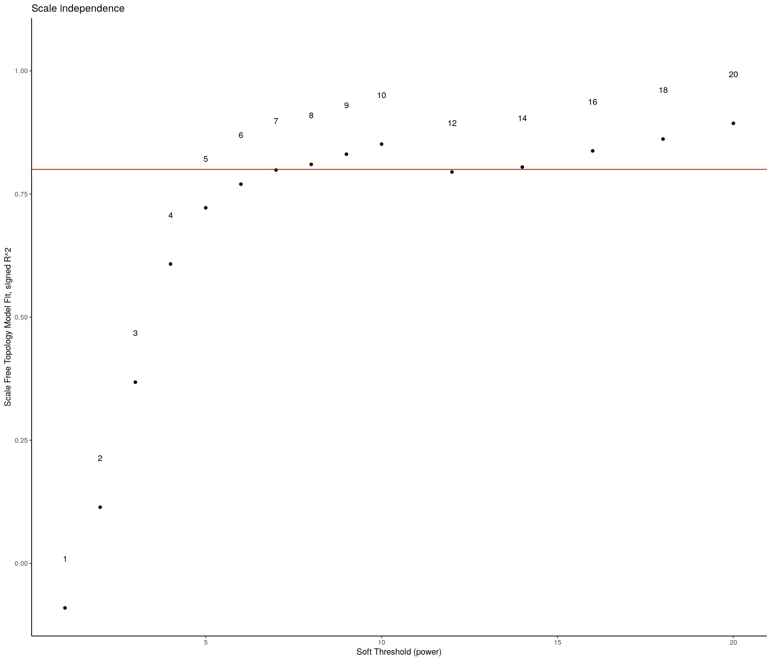
| Version | Author | Date |
|---|---|---|
| 5424b39 | xhyuo | 2023-11-06 |
#WGCNA
# temp_cor <- cor
# cor <- WGCNA::cor
# bwnet <- blockwiseModules(expression,
# networkType = "signed", # topological overlap matrix
# power = 10, # soft threshold for network construction
# # == Tree and Block Options ==
# deepSplit = 2,
# pamRespectsDendro = F,
# # detectCutHeight = 0.75,
# minModuleSize = 30,
# maxBlockSize = 4000,
# # == Module Adjustments ==
# reassignThreshold = 0,
# mergeCutHeight = 0.25,
# numericLabels = TRUE,
# randomSeed = 1234,
# verbose = 3)
# readr::write_rds(bwnet,
# file = file.path("data/BOT_NTS_rnaseq_results/wgcna/", "combined_wgcna_results.RDS")
bwnet <- readRDS("data/BOT_NTS_rnaseq_results/wgcna/combined_wgcna_results.RDS")
# Convert labels to colors for plotting
mergedColors = labels2colors(bwnet$colors)
# Plot the dendrogram and the module colors underneath
plotDendroAndColors(
bwnet$dendrograms[[1]],
mergedColors[bwnet$blockGenes[[1]]],
"Module colors",
dendroLabels = FALSE,
hang = 0.03,
addGuide = TRUE,
guideHang = 0.05 )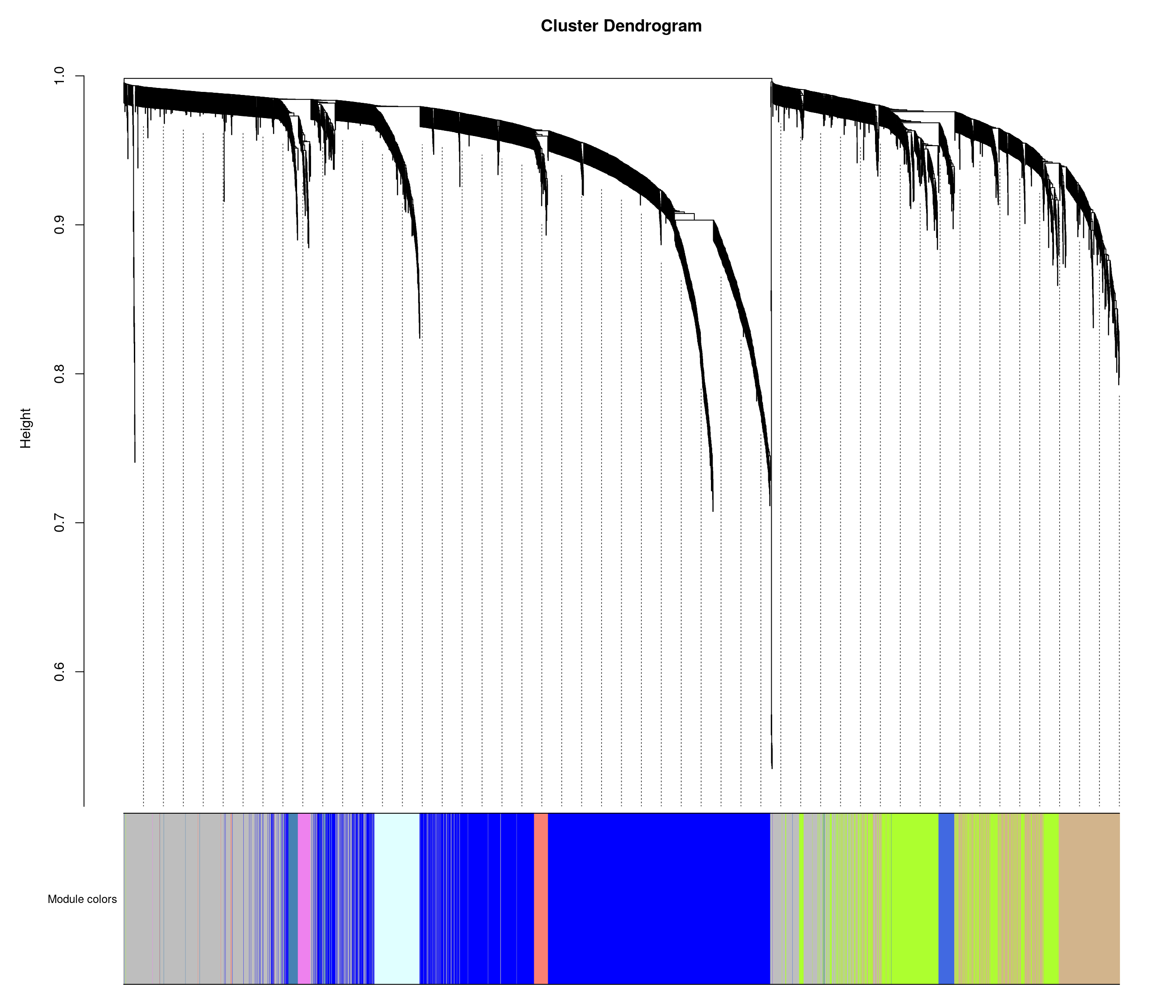
| Version | Author | Date |
|---|---|---|
| 5424b39 | xhyuo | 2023-11-06 |
#explore results
module_eigengenes <- bwnet$MEs
# Print out a preview
head(module_eigengenes) ME10 ME9 ME17 ME19 ME25
34303_BOT_F 0.047930956 0.059988733 0.0846580032 0.0176279342 0.016049071
34303_NTS_F -0.007848204 0.009410510 0.0002504076 0.0216725070 0.054054908
34304_BOT_F 0.089155926 0.109195499 0.1295135612 -0.0278529227 0.027621308
34305_BOT_M 0.026329630 0.039527611 0.0319651936 -0.0008609624 0.007713445
34305_NTS_M 0.052961927 0.027278021 0.0751157514 -0.0062885788 0.018118290
34306_BOT_M 0.033914186 0.006362045 0.0212831615 -0.0133763436 0.016397813
ME28 ME38 ME7 ME5 ME6
34303_BOT_F -0.02540143 0.03051567 -0.009108132 -0.04964410 0.003729132
34303_NTS_F 0.01847730 0.08047843 0.023522757 0.01935305 -0.004981067
34304_BOT_F -0.04075906 0.03136098 -0.021243825 -0.02648623 -0.056451997
34305_BOT_M -0.01789043 0.01654383 -0.019760573 -0.02065422 -0.039342407
34305_NTS_M 0.01664655 0.12721639 -0.003120766 0.04297403 -0.013335761
34306_BOT_M -0.02972017 0.05714328 -0.009352975 0.01061615 -0.049618686
ME13 ME14 ME29 ME43 ME30
34303_BOT_F -0.05750244 -0.015983979 -0.006926549 -0.052959188 -0.013852891
34303_NTS_F 0.06468929 0.023559930 0.010563413 -0.026514600 -0.017906234
34304_BOT_F -0.05373658 -0.001949782 -0.012071668 -0.028321907 -0.021902970
34305_BOT_M -0.06653428 -0.009266664 -0.013199115 -0.010874969 -0.006117209
34305_NTS_M 0.05669000 0.049671478 -0.018397954 0.016196191 -0.058406576
34306_BOT_M -0.05682425 -0.029478464 -0.011778218 0.001309642 -0.065830500
ME32 ME15 ME22 ME1 ME37
34303_BOT_F -0.01971730 -0.007151361 -0.006852951 -0.06139120 0.05211387
34303_NTS_F 0.05208115 -0.026694141 -0.035446418 0.02977253 0.06310212
34304_BOT_F -0.02954042 -0.018699095 -0.034621090 -0.03759643 0.05248605
34305_BOT_M -0.01881611 0.118071459 0.051607226 0.01610367 0.06921746
34305_NTS_M -0.01900677 -0.024100983 -0.033881085 -0.04494534 0.10921453
34306_BOT_M -0.03325523 -0.028806559 -0.024925596 0.02770181 0.06976949
ME2 ME16 ME21 ME26 ME4
34303_BOT_F -0.033276128 -0.012936855 0.095312364 0.05747760 -5.451119e-03
34303_NTS_F -0.004661837 -0.005741008 -0.003992772 -0.06382607 -3.003089e-02
34304_BOT_F -0.038651089 -0.018022406 0.011725645 0.06142083 -9.367489e-02
34305_BOT_M -0.041479019 -0.014151074 0.126655632 0.04635058 -9.744315e-05
34305_NTS_M 0.002959842 0.010424060 0.030088805 -0.02528155 -4.044654e-02
34306_BOT_M -0.051350350 -0.028037663 -0.021168088 -0.01116186 -2.682835e-02
ME3 ME27 ME11 ME20 ME35
34303_BOT_F 0.010440119 0.015498344 0.069797260 0.05207238 -0.0084158186
34303_NTS_F -0.039526875 -0.044225002 0.010408334 -0.02265901 0.0142861382
34304_BOT_F 0.009008827 0.005764489 0.011458811 -0.04558085 -0.0186508071
34305_BOT_M -0.014814229 0.079166656 0.065862012 0.05677946 -0.0123239058
34305_NTS_M -0.054894219 -0.031964849 -0.002037738 -0.02235332 -0.0048191863
34306_BOT_M -0.044933475 -0.029361225 0.064622276 0.02963534 0.0009305857
ME39 ME34 ME33 ME40 ME24
34303_BOT_F 0.006908751 2.074572e-02 0.009649158 0.072764628 0.003808233
34303_NTS_F 0.041918200 3.693300e-02 0.014021803 0.065825168 -0.014338493
34304_BOT_F 0.015684961 9.791089e-05 0.013820888 0.070067622 0.067495088
34305_BOT_M 0.032266935 2.299562e-02 -0.003057202 0.054944080 -0.028032206
34305_NTS_M 0.013758174 -7.484197e-02 0.061377908 -0.005464055 0.090762871
34306_BOT_M 0.041021853 3.056819e-02 0.012022543 0.068155580 0.058555419
ME42 ME8 ME23 ME12 ME18
34303_BOT_F -0.02411076 0.035293202 0.050835110 0.043420094 0.06385463
34303_NTS_F -0.02109214 -0.026201009 -0.014000314 0.014048735 -0.05412699
34304_BOT_F 0.02177225 0.030832695 0.097635991 0.067731278 0.08541624
34305_BOT_M -0.05864474 -0.003325469 -0.008550676 0.008620296 0.02562227
34305_NTS_M 0.02625905 -0.040495191 0.077395519 0.047346773 -0.07314033
34306_BOT_M 0.01688917 0.033347781 0.061603702 0.082622687 0.02859475
ME36 ME31 ME41 ME0
34303_BOT_F 0.03150222 0.015315662 -0.03032894 -0.036816725
34303_NTS_F -0.04374266 0.009696843 -0.02688429 0.038117895
34304_BOT_F 0.00613193 0.013477583 -0.03093792 -0.042865628
34305_BOT_M -0.02675624 0.014546240 -0.03168659 -0.011243224
34305_NTS_M -0.09071419 -0.038939859 -0.03381559 -0.026170703
34306_BOT_M 0.01347904 0.040345797 -0.02764635 -0.001750545#Which modules have biggest differences across strain?
all.equal(rownames(df), rownames(module_eigengenes))[1] TRUE# Create the design matrix from the `time_point` variable
des_mat <- model.matrix(~ df$Strain)
# lmFit() needs a transposed version of the matrix
fit <- limma::lmFit(t(module_eigengenes), design = des_mat)
# Apply empirical Bayes to smooth standard errors
fit <- limma::eBayes(fit)
# Apply multiple testing correction and obtain stats
stats_df <- limma::topTable(fit, number = ncol(module_eigengenes)) %>%
tibble::rownames_to_column("module")Removing intercept from test coefficients#head(stats_df)
#display stats_df
DT::datatable(stats_df,
filter = list(position = 'top', clear = FALSE),
extensions = 'Buttons',
options = list(dom = 'Blfrtip',
buttons = c('csv', 'excel'),
lengthMenu = list(c(10,25,50,-1),
c(10,25,50,"All")),
pageLength = 40,
scrollY = "300px",
scrollX = "40px"),
caption = htmltools::tags$caption(style = 'caption-side: top; text-align: left; color:black; font-size:200% ;',
'Modules differences across strain'))module_df <- module_eigengenes %>%
tibble::rownames_to_column("Name") %>%
# Here we are performing an inner join with a subset of metadata
dplyr::inner_join(df %>%
tibble::rownames_to_column("Name")
)Joining, by = "Name"#plot of module
ggplot(
module_df,
aes_string(
x = "Strain",
y = stats_df[1,"module"],
color = "Strain"
)
) +
# a boxplot with outlier points hidden (they will be in the sina plot)
geom_boxplot(width = 0.2, outlier.shape = NA) +
# A sina plot to show all of the individual data points
ggforce::geom_sina(maxwidth = 0.3) +
theme_classic() +
theme(legend.position = "none",
axis.text.x = element_text(angle = 90, vjust = 0.5, hjust=1))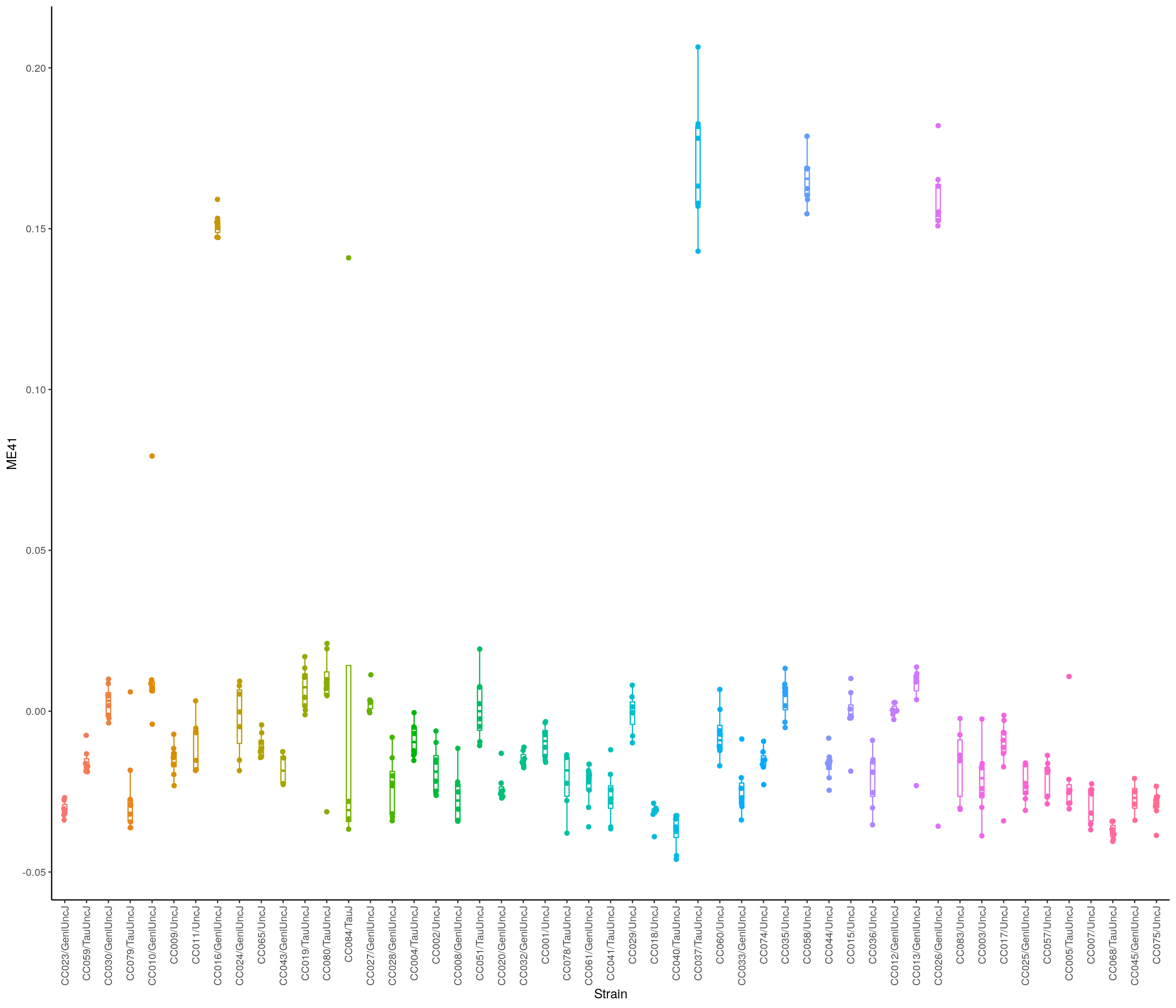
#hub genes
hubs = chooseTopHubInEachModule(expression, bwnet$colors)
hubs_df = data.frame(hubgene = hubs, mark_hub_gene_in_module = paste0("ME", names(hubs)))
#gene content
gene_module_key <- tibble::enframe(bwnet$colors, name = "gene", value = "module") %>%
# Let's add the `ME` part so its more clear what these numbers are and it matches elsewhere
dplyr::mutate(module = paste0("ME", module)) %>%
dplyr::left_join(genes, by = c("gene" = "ENSEMBL")) %>%
dplyr::left_join(hubs_df, by = c("gene" = "hubgene"))
#display stats_df
DT::datatable(gene_module_key,
filter = list(position = 'top', clear = FALSE),
extensions = 'Buttons',
options = list(dom = 'Blfrtip',
buttons = c('csv', 'excel'),
lengthMenu = list(c(10,25,50,-1),
c(10,25,50,"All")),
pageLength = 40,
scrollY = "300px",
scrollX = "40px"),
caption = htmltools::tags$caption(style = 'caption-side: top; text-align: left; color:black; font-size:200% ;',
'Module gene content'))Warning in instance$preRenderHook(instance): It seems your data is too big
for client-side DataTables. You may consider server-side processing: https://
rstudio.github.io/DT/server.html# for(m in stats_df$module[1:10]){
# mod_heatmap <- make_module_heatmap(module_name = m,
# expression_mat = expression,
# metadata_df = df,
# gene_module_key_df = gene_module_key,
# module_eigengenes_df = module_eigengenes
# )
# pdf(paste0("data/BOT_NTS_rnaseq_results/wgcna/combined_module_", m, ".pdf"), width = 14, height = 12)
# mod_heatmap <- make_module_heatmap(module_name = m,
# expression_mat = expression,
# metadata_df = df,
# gene_module_key_df = gene_module_key,
# module_eigengenes_df = module_eigengenes
# )
# mod_heatmap
# dev.off()
# }
nGenes = ncol(expression)
nSamples = nrow(expression)
MEs0 <- moduleEigengenes(expression, gsub("ME", "", gene_module_key$module))$eigengenes
MEs <- orderMEs(MEs0)
corType = "pearson"
robustY = ifelse(corType=="pearson",T,F)
all.equal(rownames(MEs), (design.matrix.pheno$name))[1] TRUEmodCor = cor(MEs, design.matrix.pheno[,colnames(design.matrix.pheno)[27:176]], use = "p")
modCor = modCor[,colSums(!is.na(modCor)) > 0]
modP = corPvalueStudent(modCor, nSamples)
modP = modP[,colSums(!is.na(modP)) > 0]
modCor_results <- as.data.frame(modCor)
modadjustP_results <- as.data.frame(modP) %>%
dplyr::mutate(across(.cols = everything(), ~p.adjust(.x, method = "fdr")))
#display modCor_results
DT::datatable(modCor_results,
filter = list(position = 'top', clear = FALSE),
extensions = 'Buttons',
options = list(dom = 'Blfrtip',
buttons = c('csv', 'excel'),
lengthMenu = list(c(10,25,50,-1),
c(10,25,50,"All")),
pageLength = 40,
scrollY = "300px",
scrollX = "40px"),
caption = htmltools::tags$caption(style = 'caption-side: top; text-align: left; color:black; font-size:200% ;',
'Module-phenotype correlation'))#display modadjustP_results
DT::datatable(modadjustP_results,
filter = list(position = 'top', clear = FALSE),
extensions = 'Buttons',
options = list(dom = 'Blfrtip',
buttons = c('csv', 'excel'),
lengthMenu = list(c(10,25,50,-1),
c(10,25,50,"All")),
pageLength = 40,
scrollY = "300px",
scrollX = "40px"),
caption = htmltools::tags$caption(style = 'caption-side: top; text-align: left; color:black; font-size:200% ;',
'Adjusted p values for module-phenotype correlation'))WGCNA for BOT datasets
load("data/BOT_NTS_rnaseq_results/rld.RData")
expression = t(assay(rld))
all.equal(rownames(df), rownames(expression))[1] TRUE#BOT
expression <- expression[rownames(df[df$Tissue == "BOT",]),]
#Determine parameters for WGCNA
sft <- pickSoftThreshold(expression,
dataIsExpr = TRUE,
corFnc = cor,
networkType = "signed"
) Power SFT.R.sq slope truncated.R.sq mean.k. median.k. max.k.
1 1 0.0147 -12.80 0.937 10800.00 1.08e+04 11200.0
2 2 0.5380 -43.20 0.932 5540.00 5.52e+03 6030.0
3 3 0.6650 -21.90 0.925 2890.00 2.86e+03 3400.0
4 4 0.7770 -12.50 0.965 1540.00 1.51e+03 2000.0
5 5 0.8320 -9.03 0.985 835.00 8.10e+02 1240.0
6 6 0.8530 -6.92 0.988 462.00 4.41e+02 808.0
7 7 0.8700 -5.53 0.990 262.00 2.44e+02 551.0
8 8 0.8870 -4.57 0.991 152.00 1.37e+02 392.0
9 9 0.8960 -3.91 0.988 90.00 7.77e+01 290.0
10 10 0.9070 -3.43 0.988 54.80 4.48e+01 222.0
11 12 0.9250 -2.79 0.988 22.00 1.55e+01 143.0
12 14 0.9410 -2.40 0.987 9.88 5.69e+00 101.0
13 16 0.9560 -2.12 0.988 4.93 2.19e+00 76.2
14 18 0.9690 -1.94 0.991 2.72 8.84e-01 60.0
15 20 0.9750 -1.81 0.989 1.63 3.75e-01 48.7sft_df <- data.frame(sft$fitIndices) %>%
dplyr::mutate(model_fit = -sign(slope) * SFT.R.sq)
ggplot(sft_df, aes(x = Power, y = model_fit, label = Power)) +
# Plot the points
geom_point() +
# We'll put the Power labels slightly above the data points
geom_text(nudge_y = 0.1) +
# We will plot what WGCNA recommends as an R^2 cutoff
geom_hline(yintercept = 0.80, col = "red") +
# Just in case our values are low, we want to make sure we can still see the 0.80 level
ylim(c(min(sft_df$model_fit), 1.05)) +
# We can add more sensible labels for our axis
xlab("Soft Threshold (power)") +
ylab("Scale Free Topology Model Fit, signed R^2") +
ggtitle("Scale independence") +
# This adds some nicer aesthetics to our plot
theme_classic()Warning: Removed 3 rows containing missing values (geom_text).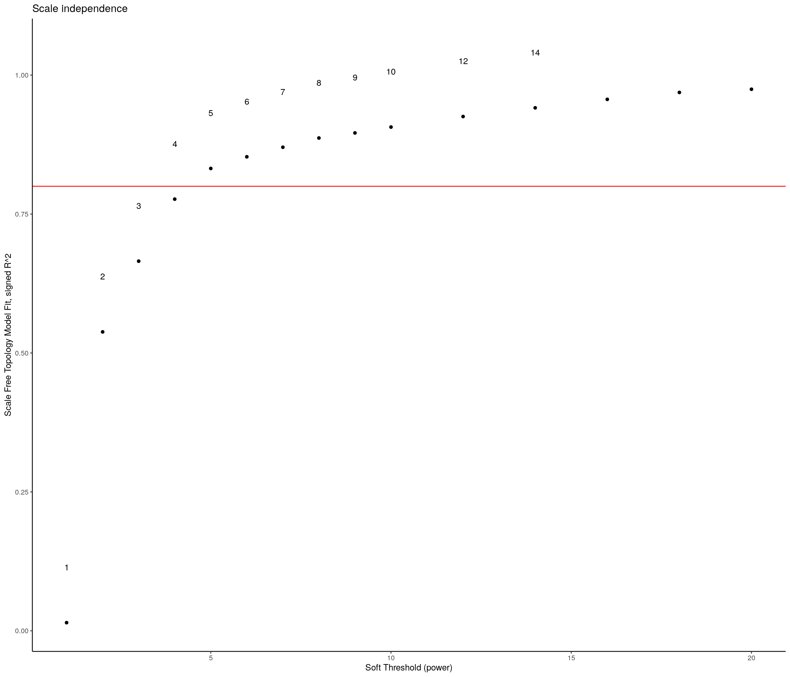
| Version | Author | Date |
|---|---|---|
| 5424b39 | xhyuo | 2023-11-06 |
#WGCNA
# temp_cor <- cor
# cor <- WGCNA::cor
# bwnet <- blockwiseModules(expression,
# networkType = "signed", # topological overlap matrix
# power = 10, # soft threshold for network construction
# # == Tree and Block Options ==
# deepSplit = 2,
# pamRespectsDendro = F,
# # detectCutHeight = 0.75,
# minModuleSize = 30,
# maxBlockSize = 4000,
# # == Module Adjustments ==
# reassignThreshold = 0,
# mergeCutHeight = 0.25,
# numericLabels = TRUE,
# randomSeed = 1234,
# verbose = 3)
# readr::write_rds(bwnet,
# file = file.path("data/BOT_NTS_rnaseq_results/wgcna/", "BOT_wgcna_results.RDS")
# )
bwnet <- readRDS("data/BOT_NTS_rnaseq_results/wgcna/BOT_wgcna_results.RDS")
# Convert labels to colors for plotting
mergedColors = labels2colors(bwnet$colors)
# Plot the dendrogram and the module colors underneath
plotDendroAndColors(
bwnet$dendrograms[[1]],
mergedColors[bwnet$blockGenes[[1]]],
"Module colors",
dendroLabels = FALSE,
hang = 0.03,
addGuide = TRUE,
guideHang = 0.05 )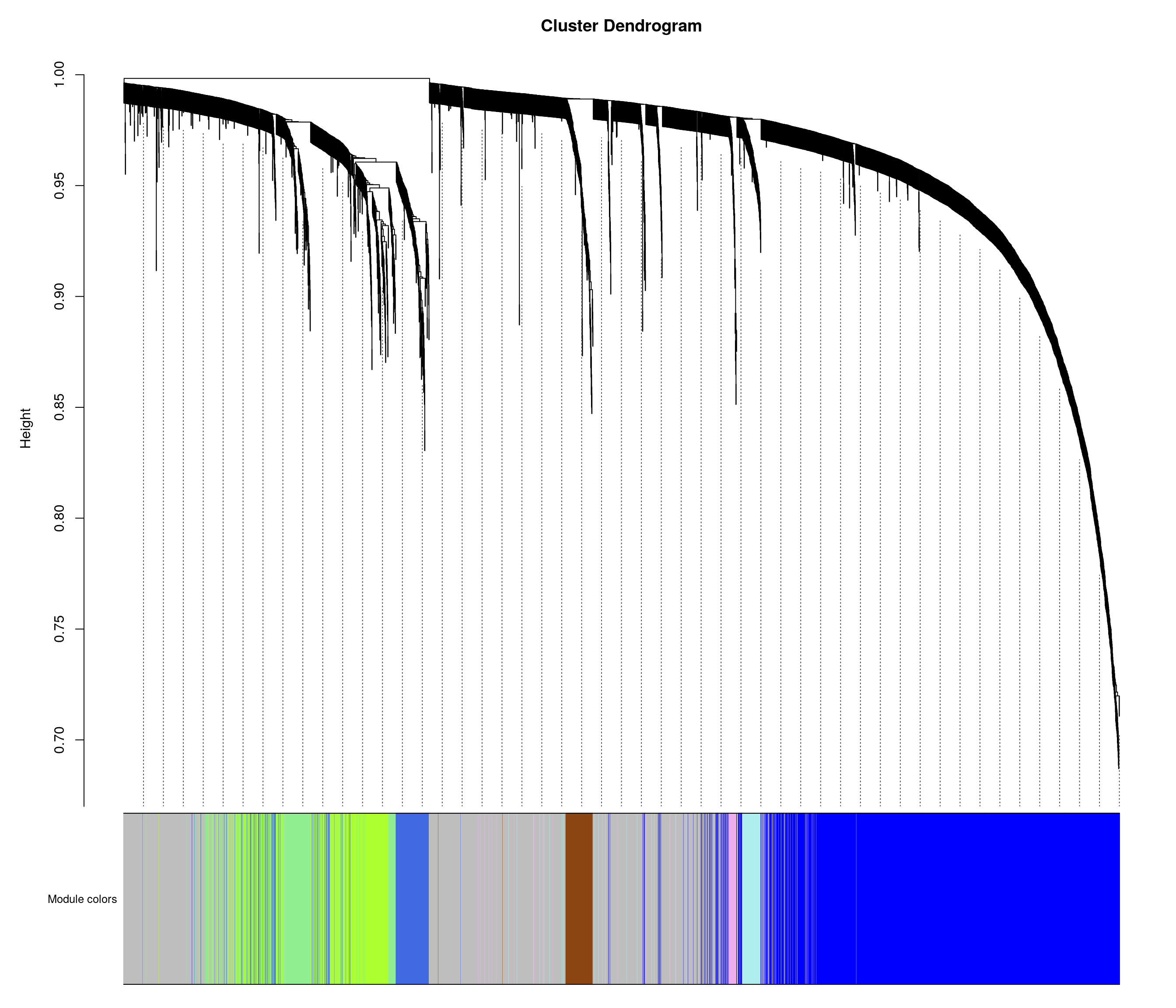
| Version | Author | Date |
|---|---|---|
| 5424b39 | xhyuo | 2023-11-06 |
#explore results
module_eigengenes <- bwnet$MEs
# Print out a preview
head(module_eigengenes) ME13 ME27 ME8 ME19 ME50
34303_BOT_F 0.10124996 0.09105329 0.03974511 0.06317376 0.10429040
34304_BOT_F 0.03771612 0.21297725 0.09570031 0.15018480 0.10936512
34305_BOT_M 0.11077416 0.04465883 0.01665237 0.02395634 0.08197325
34306_BOT_M 0.03756751 -0.08409431 -0.03747676 0.00129071 0.10155612
35442_BOT_F 0.13050526 0.08239896 0.03490488 0.03862987 0.07758907
35443_BOT_F -0.27878733 -0.11065642 -0.17603314 -0.26874933 0.15045639
ME52 ME53 ME11 ME37 ME10
34303_BOT_F 0.026553940 -0.02313406 0.11992533 0.06988045 -0.011668305
34304_BOT_F 0.021684435 -0.02213552 0.10619492 0.07931035 -0.006077209
34305_BOT_M 0.007753284 -0.02498062 0.03769735 -0.05053102 -0.046939767
34306_BOT_M 0.023078485 -0.02905579 0.12298805 0.02717356 0.061908224
35442_BOT_F 0.076365030 -0.02155856 0.01561649 -0.04187468 -0.025461018
35443_BOT_F 0.028055531 -0.00624761 0.05249210 0.22359609 -0.189034993
ME20 ME42 ME17 ME18 ME30
34303_BOT_F 0.10277513 0.007491512 0.06195935 0.13413920 0.075395397
34304_BOT_F 0.04132318 0.108103496 0.13294798 0.21139066 0.161574279
34305_BOT_M 0.05832487 -0.058047794 -0.00477231 0.03777935 -0.005133931
34306_BOT_M 0.12175895 0.105910771 0.10264418 0.10469144 0.052800454
35442_BOT_F 0.04896319 -0.117816525 -0.03329155 -0.03317235 -0.045263945
35443_BOT_F -0.18587361 0.196376361 -0.13146857 0.04047521 0.061512251
ME3 ME24 ME36 ME47 ME55
34303_BOT_F -0.04545070 0.066708319 0.07263105 0.04215744 -0.20156887
34304_BOT_F -0.05876409 0.064629570 0.02189064 0.03033514 -0.19849036
34305_BOT_M -0.07182944 -0.036267350 0.06462567 0.04889615 -0.20713727
34306_BOT_M -0.05747033 0.076062119 0.04132999 0.06240371 -0.21013426
35442_BOT_F -0.01162274 0.003108767 0.08435681 0.03798336 0.05766089
35443_BOT_F -0.05213101 0.043114494 -0.03638483 0.03466022 0.02398880
ME32 ME44 ME28 ME39 ME33
34303_BOT_F -0.0016213102 0.04474993 -0.030133244 -0.082727748 -0.096026624
34304_BOT_F -0.0198375831 0.05509846 0.080681169 -0.009543601 -0.078235826
34305_BOT_M -0.0028172450 0.04648956 -0.097199204 -0.125990763 -0.034359477
34306_BOT_M -0.0006028658 0.05931209 -0.008956397 -0.034990209 -0.007534424
35442_BOT_F -0.0399591465 0.02787388 -0.119768245 -0.098001070 -0.082297473
35443_BOT_F -0.0418366420 0.01790937 0.078149271 -0.138528278 -0.070724642
ME22 ME16 ME26 ME29 ME31
34303_BOT_F -0.08935262 -0.06252677 0.006321099 0.020465230 0.001120670
34304_BOT_F -0.04475929 -0.06077997 0.024856168 -0.048402757 0.025719297
34305_BOT_M -0.12511506 -0.07719541 -0.022429013 -0.003755404 -0.010775958
34306_BOT_M -0.08739020 -0.05600060 0.066634088 -0.020932329 0.009589668
35442_BOT_F -0.10722191 -0.06820015 -0.053729909 -0.003481886 -0.122728484
35443_BOT_F -0.06773980 -0.03395661 -0.107653043 0.016870136 -0.078239978
ME40 ME41 ME2 ME23 ME49
34303_BOT_F 0.008997586 -0.0275139176 -0.04031311 -0.040013298 -0.11968934
34304_BOT_F -0.073043794 -0.0793714960 -0.09805437 -0.080754843 -0.10019563
34305_BOT_M 0.078328081 0.0107054550 -0.08445867 0.029943873 -0.06833842
34306_BOT_M -0.087060857 -0.0004446998 -0.09790449 -0.102384673 -0.06689718
35442_BOT_F 0.099406591 0.0812294172 -0.06773304 0.006078434 -0.02208815
35443_BOT_F -0.189604170 -0.3395961997 -0.01271783 0.056921490 -0.16708650
ME6 ME34 ME43 ME54 ME48
34303_BOT_F -0.13673549 -0.073551094 0.04646859 -0.008019553 -0.01997440
34304_BOT_F -0.09186848 -0.033072584 0.04171161 -0.019594626 -0.04461392
34305_BOT_M -0.09956732 -0.041745833 0.04758757 0.023755861 -0.02612552
34306_BOT_M -0.03434642 -0.104985733 0.08289223 0.015138173 -0.04193189
35442_BOT_F -0.04104439 -0.003829921 -0.02513485 0.020988934 0.13060358
35443_BOT_F -0.19972731 -0.245836202 -0.03376041 0.032175775 0.13672192
ME38 ME51 ME9 ME12 ME4
34303_BOT_F 0.02780532 -0.03558556 0.13134015 0.1271851056 0.000301173
34304_BOT_F 0.03268491 -0.04846678 0.08373324 0.0534458329 -0.007444862
34305_BOT_M 0.04770148 -0.04386779 0.09331849 0.1558109598 0.102845381
34306_BOT_M 0.03907122 -0.02665394 0.03566189 -0.0003473564 -0.040229314
35442_BOT_F 0.05217609 0.05106292 0.05022894 0.0061564447 0.094635930
35443_BOT_F 0.06404160 0.02174137 0.19807686 0.0610795052 0.073412905
ME5 ME1 ME14 ME21 ME25
34303_BOT_F 0.05884156 -0.06342143 -0.12535223 0.01677805 0.0075683594
34304_BOT_F 0.04121209 -0.02571491 -0.03674449 0.02164955 0.1021848814
34305_BOT_M 0.05102010 0.04646515 -0.04401159 -0.04934198 -0.0161334742
34306_BOT_M -0.03497622 0.07174478 0.01491386 -0.08596997 -0.0002655557
35442_BOT_F 0.06581771 0.01190851 -0.09767429 -0.04447881 -0.0742002058
35443_BOT_F 0.15265793 0.24069076 0.27923545 0.37116777 0.3609798649
ME7 ME15 ME35 ME45 ME46
34303_BOT_F -0.02033830 0.08598849 0.09441604 0.004949691 0.08418004
34304_BOT_F -0.14847240 -0.09801058 -0.12995723 0.010066550 0.08547913
34305_BOT_M 0.02326416 0.09321244 0.03493084 0.027298671 0.09403176
34306_BOT_M -0.02191984 0.03612091 0.04491648 0.043502250 0.09940955
35442_BOT_F 0.02932159 0.12304521 0.04354694 0.042758970 0.11626789
35443_BOT_F 0.08296718 -0.12102056 0.13693768 0.015383259 0.09644972
ME0
34303_BOT_F 0.03084068
34304_BOT_F 0.03194201
34305_BOT_M 0.04136509
34306_BOT_M 0.07947080
35442_BOT_F 0.02430419
35443_BOT_F 0.26617092#Which modules have biggest differences across strain?
all.equal(rownames(df[df$Tissue == "BOT",]), rownames(module_eigengenes))[1] TRUE# Create the design matrix from the `time_point` variable
des_mat <- model.matrix(~ df[df$Tissue == "BOT",]$Strain)
# lmFit() needs a transposed version of the matrix
fit <- limma::lmFit(t(module_eigengenes), design = des_mat)
# Apply empirical Bayes to smooth standard errors
fit <- limma::eBayes(fit)
# Apply multiple testing correction and obtain stats
stats_df <- limma::topTable(fit, number = ncol(module_eigengenes)) %>%
tibble::rownames_to_column("module")Removing intercept from test coefficients#head(stats_df)
colnames(stats_df) = sub('.*Strain', '', colnames(stats_df))
#display stats_df
DT::datatable(stats_df,
filter = list(position = 'top', clear = FALSE),
extensions = 'Buttons',
options = list(dom = 'Blfrtip',
buttons = c('csv', 'excel'),
lengthMenu = list(c(10,25,50,-1),
c(10,25,50,"All")),
pageLength = 40,
scrollY = "300px",
scrollX = "40px"),
caption = htmltools::tags$caption(style = 'caption-side: top; text-align: left; color:black; font-size:200% ;',
'Modules differences across strain in BOT'))module_df <- module_eigengenes %>%
tibble::rownames_to_column("Name") %>%
# Here we are performing an inner join with a subset of metadata
dplyr::inner_join(df %>%
tibble::rownames_to_column("Name")
)Joining, by = "Name"#plot of module
ggplot(
module_df,
aes_string(
x = "Strain",
y = stats_df[1,"module"],
color = "Strain"
)
) +
# a boxplot with outlier points hidden (they will be in the sina plot)
geom_boxplot(width = 0.2, outlier.shape = NA) +
# A sina plot to show all of the individual data points
ggforce::geom_sina(maxwidth = 0.3) +
theme_classic() +
theme(legend.position = "none",
axis.text.x = element_text(angle = 90, vjust = 0.5, hjust=1))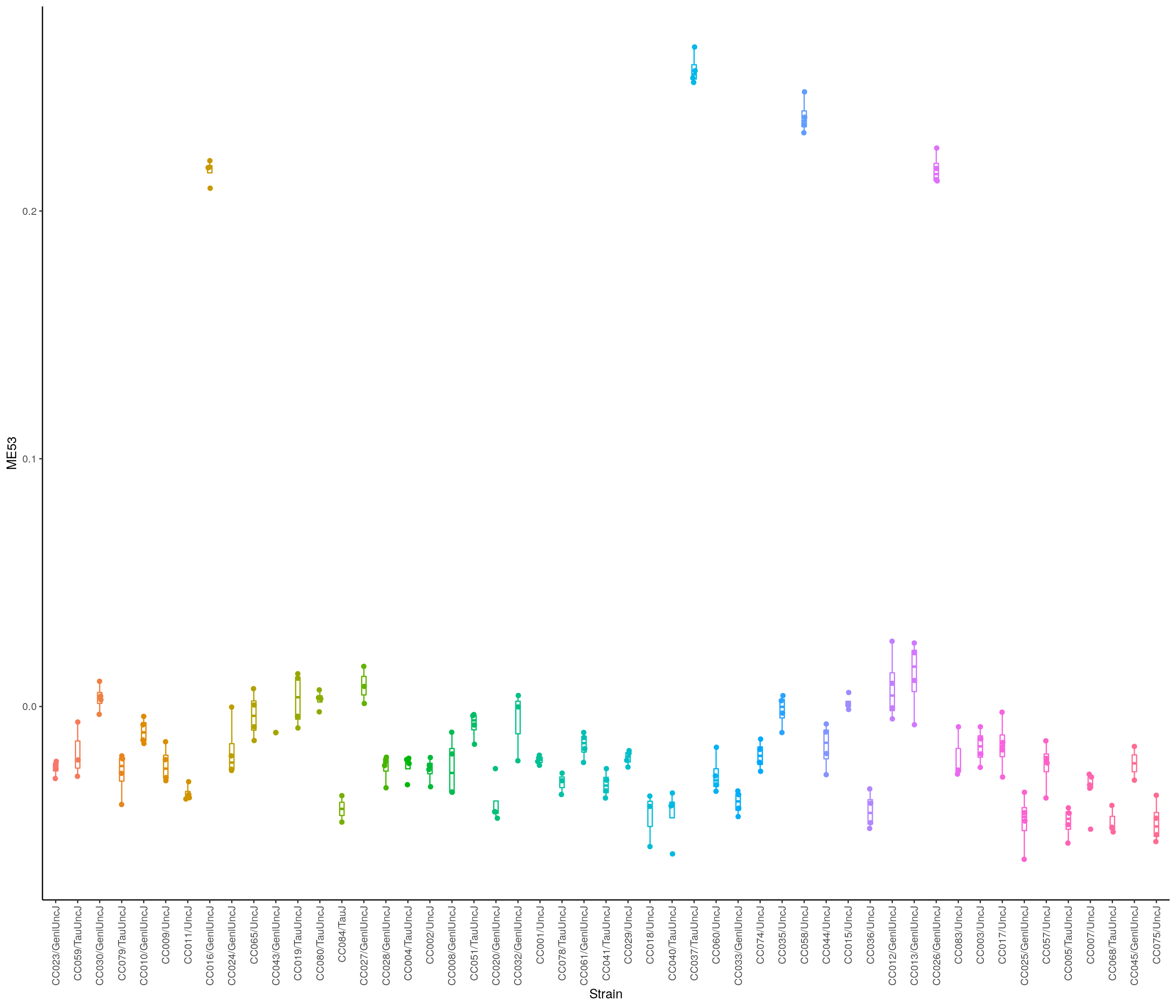
#hub genes
hubs = chooseTopHubInEachModule(expression, bwnet$colors)
hubs_df = data.frame(hubgene = hubs, mark_hub_gene_in_module = paste0("ME", names(hubs)))
#gene content
gene_module_key <- tibble::enframe(bwnet$colors, name = "gene", value = "module") %>%
# Let's add the `ME` part so its more clear what these numbers are and it matches elsewhere
dplyr::mutate(module = paste0("ME", module)) %>%
dplyr::left_join(genes, by = c("gene" = "ENSEMBL")) %>%
dplyr::left_join(hubs_df, by = c("gene" = "hubgene"))
#display stats_df
DT::datatable(gene_module_key,
filter = list(position = 'top', clear = FALSE),
extensions = 'Buttons',
options = list(dom = 'Blfrtip',
buttons = c('csv', 'excel'),
lengthMenu = list(c(10,25,50,-1),
c(10,25,50,"All")),
pageLength = 40,
scrollY = "300px",
scrollX = "40px"),
caption = htmltools::tags$caption(style = 'caption-side: top; text-align: left; color:black; font-size:200% ;',
'Module gene content'))Warning in instance$preRenderHook(instance): It seems your data is too big
for client-side DataTables. You may consider server-side processing: https://
rstudio.github.io/DT/server.htmlnGenes = ncol(expression)
nSamples = nrow(expression)
MEs0 <- moduleEigengenes(expression, gsub("ME", "", gene_module_key$module))$eigengenes
MEs <- orderMEs(MEs0)
corType = "pearson"
robustY = ifelse(corType=="pearson",T,F)
all.equal(rownames(MEs), (design.matrix.pheno[rownames(df[df$Tissue == "BOT",]),]$name))[1] TRUEmodCor = cor(MEs, design.matrix.pheno[rownames(df[df$Tissue == "BOT",]),][,colnames(design.matrix.pheno)[27:176]], use = "p")
modCor = modCor[,colSums(!is.na(modCor)) > 0]
modP = corPvalueStudent(modCor, nSamples)
modP = modP[,colSums(!is.na(modP)) > 0]
modCor_results <- as.data.frame(modCor)
modadjustP_results <- as.data.frame(modP) %>%
dplyr::mutate(across(.cols = everything(), ~p.adjust(.x, method = "fdr")))
#display modCor_results
DT::datatable(modCor_results,
filter = list(position = 'top', clear = FALSE),
extensions = 'Buttons',
options = list(dom = 'Blfrtip',
buttons = c('csv', 'excel'),
lengthMenu = list(c(10,25,50,-1),
c(10,25,50,"All")),
pageLength = 40,
scrollY = "300px",
scrollX = "40px"),
caption = htmltools::tags$caption(style = 'caption-side: top; text-align: left; color:black; font-size:200% ;',
'Module-phenotype correlation'))#display modadjustP_results
DT::datatable(modadjustP_results,
filter = list(position = 'top', clear = FALSE),
extensions = 'Buttons',
options = list(dom = 'Blfrtip',
buttons = c('csv', 'excel'),
lengthMenu = list(c(10,25,50,-1),
c(10,25,50,"All")),
pageLength = 40,
scrollY = "300px",
scrollX = "40px"),
caption = htmltools::tags$caption(style = 'caption-side: top; text-align: left; color:black; font-size:200% ;',
'Adjusted p values for module-phenotype correlation'))WGCNA for NTS datasets
load("data/BOT_NTS_rnaseq_results/rld.RData")
expression = t(assay(rld))
all.equal(rownames(df), rownames(expression))[1] TRUE#NTS
expression <- expression[rownames(df[df$Tissue == "NTS",]),]
#Determine parameters for WGCNA
sft <- pickSoftThreshold(expression,
dataIsExpr = TRUE,
corFnc = cor,
networkType = "signed"
) Power SFT.R.sq slope truncated.R.sq mean.k. median.k. max.k.
1 1 0.0550 14.60 0.958 10900.00 1.09e+04 11300.0
2 2 0.0674 -7.22 0.882 5600.00 5.58e+03 6240.0
3 3 0.3360 -9.41 0.831 2950.00 2.92e+03 3650.0
4 4 0.5620 -8.22 0.860 1590.00 1.56e+03 2250.0
5 5 0.7300 -6.73 0.913 875.00 8.53e+02 1460.0
6 6 0.8450 -5.62 0.956 494.00 4.73e+02 987.0
7 7 0.8990 -4.74 0.977 285.00 2.67e+02 696.0
8 8 0.9230 -4.10 0.985 169.00 1.53e+02 513.0
9 9 0.9350 -3.68 0.988 102.00 8.90e+01 395.0
10 10 0.9400 -3.32 0.988 63.90 5.25e+01 315.0
11 12 0.9400 -2.83 0.985 27.00 1.90e+01 215.0
12 14 0.9140 -2.55 0.968 12.70 7.30e+00 157.0
13 16 0.9080 -2.31 0.960 6.65 2.95e+00 121.0
14 18 0.9170 -2.13 0.965 3.80 1.25e+00 95.6
15 20 0.9240 -1.97 0.966 2.34 5.52e-01 77.6sft_df <- data.frame(sft$fitIndices) %>%
dplyr::mutate(model_fit = -sign(slope) * SFT.R.sq)
ggplot(sft_df, aes(x = Power, y = model_fit, label = Power)) +
# Plot the points
geom_point() +
# We'll put the Power labels slightly above the data points
geom_text(nudge_y = 0.1) +
# We will plot what WGCNA recommends as an R^2 cutoff
geom_hline(yintercept = 0.80, col = "red") +
# Just in case our values are low, we want to make sure we can still see the 0.80 level
ylim(c(min(sft_df$model_fit), 1.05)) +
# We can add more sensible labels for our axis
xlab("Soft Threshold (power)") +
ylab("Scale Free Topology Model Fit, signed R^2") +
ggtitle("Scale independence") +
# This adds some nicer aesthetics to our plot
theme_classic()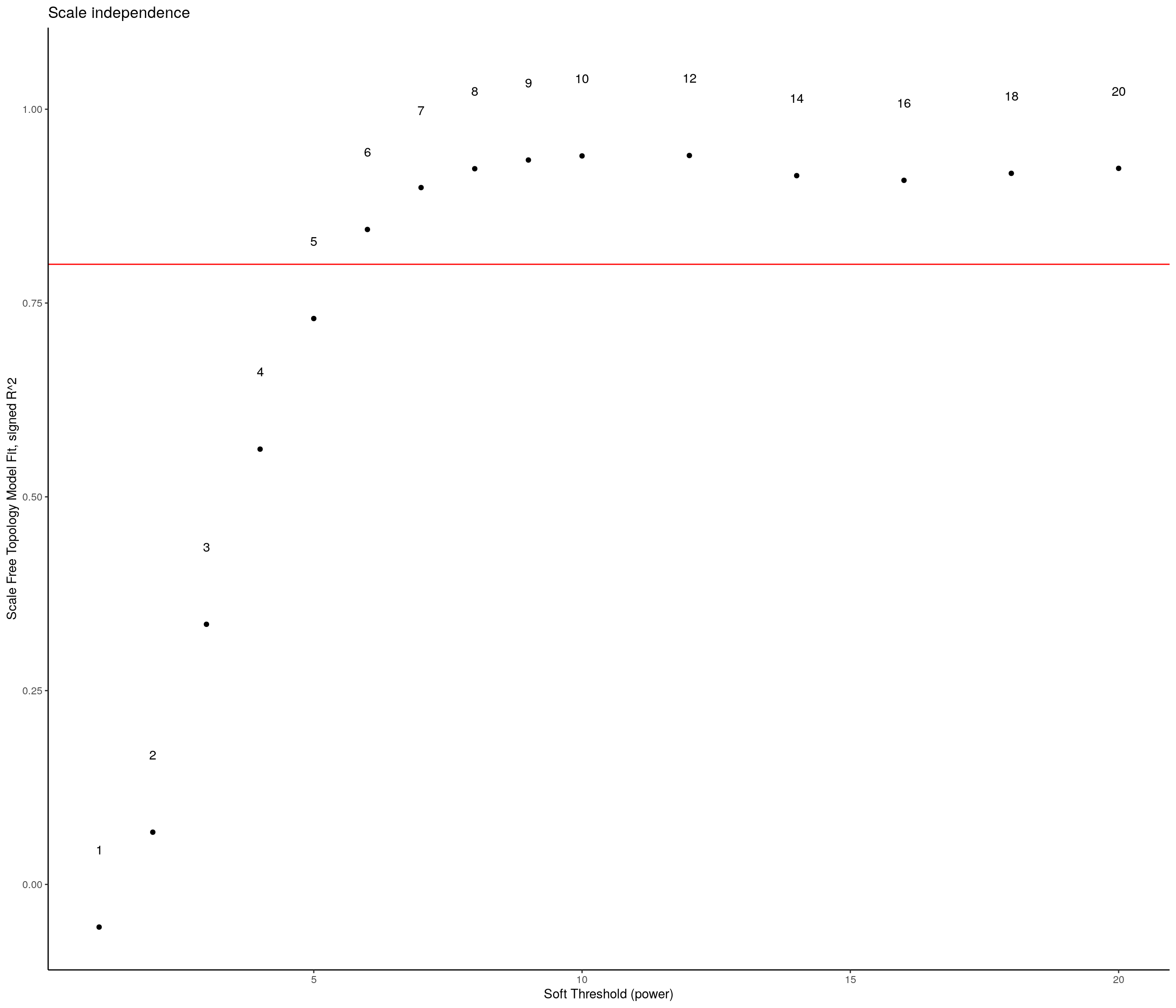
| Version | Author | Date |
|---|---|---|
| 5424b39 | xhyuo | 2023-11-06 |
#WGCNA
# temp_cor <- cor
# cor <- WGCNA::cor
# bwnet <- blockwiseModules(expression,
# networkType = "signed", # topological overlap matrix
# power = 10, # soft threshold for network construction
# # == Tree and Block Options ==
# deepSplit = 2,
# pamRespectsDendro = F,
# # detectCutHeight = 0.75,
# minModuleSize = 30,
# maxBlockSize = 4000,
# # == Module Adjustments ==
# reassignThreshold = 0,
# mergeCutHeight = 0.25,
# numericLabels = TRUE,
# randomSeed = 1234,
# verbose = 3)
# readr::write_rds(bwnet,
# file = file.path("data/BOT_NTS_rnaseq_results/wgcna/", "NTS_wgcna_results.RDS")
# )
bwnet <- readRDS("data/BOT_NTS_rnaseq_results/wgcna/NTS_wgcna_results.RDS")
# Convert labels to colors for plotting
mergedColors = labels2colors(bwnet$colors)
# Plot the dendrogram and the module colors underneath
plotDendroAndColors(
bwnet$dendrograms[[1]],
mergedColors[bwnet$blockGenes[[1]]],
"Module colors",
dendroLabels = FALSE,
hang = 0.03,
addGuide = TRUE,
guideHang = 0.05 )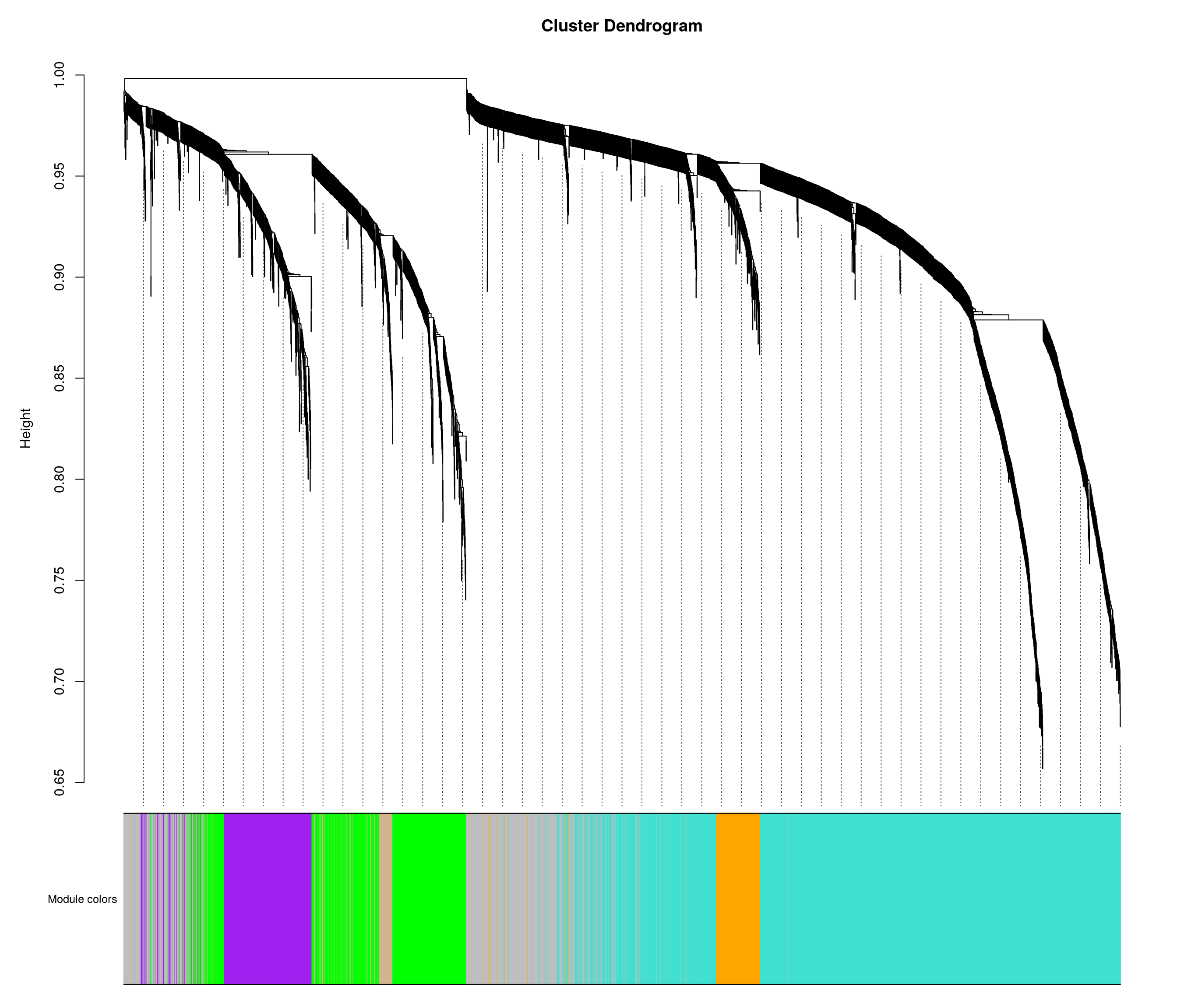
| Version | Author | Date |
|---|---|---|
| 5424b39 | xhyuo | 2023-11-06 |
#explore results
module_eigengenes <- bwnet$MEs
# Print out a preview
head(module_eigengenes) ME41 ME12 ME21 ME6 ME34
34303_NTS_F 0.01722966 0.033300563 -0.04915371 -0.079411688 -0.13130415
34305_NTS_M -0.06377499 0.028527335 -0.04308696 -0.103680088 -0.15459064
34306_NTS_M 0.02913916 0.057276400 0.01922020 -0.009580588 -0.02314573
35442_NTS_F -0.04604294 0.007065228 -0.00170309 -0.065487344 -0.14059304
35443_NTS_F -0.02984199 -0.001623035 -0.02562947 -0.016700309 -0.01701392
35444_NTS_M -0.03496079 0.038689056 -0.01012328 -0.024633731 -0.07121828
ME24 ME33 ME27 ME14 ME1
34303_NTS_F 0.043825522 0.11372306 0.002334411 0.02593962 -0.009500823
34305_NTS_M 0.007821914 0.05058209 -0.026120346 -0.03661395 -0.001591215
34306_NTS_M 0.032862065 0.14952629 0.027014229 -0.03418958 -0.037355128
35442_NTS_F 0.029074612 -0.08814260 -0.005747082 -0.02398793 -0.030179892
35443_NTS_F 0.013676381 -0.10350555 -0.037984993 -0.04773174 -0.035187941
35444_NTS_M 0.018239937 -0.07806151 -0.018228779 -0.01549241 -0.005060563
ME18 ME25 ME38 ME9 ME19
34303_NTS_F 0.016133091 0.07379931 -0.02586015 -0.012313188 -0.091793510
34305_NTS_M 0.007218905 0.06400924 -0.07054234 -0.007436589 -0.122624426
34306_NTS_M -0.016612661 -0.01163148 -0.04924395 -0.022644662 -0.039709748
35442_NTS_F -0.045614608 -0.02291461 -0.01812557 -0.040416549 -0.127616286
35443_NTS_F -0.087676009 -0.07088759 0.03405859 -0.024858647 -0.004946265
35444_NTS_M -0.008008742 0.01444546 0.02303734 -0.015644277 -0.058607063
ME2 ME36 ME44 ME16 ME46
34303_NTS_F 0.023804648 -0.04768928 0.07939730 0.0286531895 0.072482309
34305_NTS_M -0.081528700 -0.07308488 -0.12719542 -0.0397125152 0.030064085
34306_NTS_M -0.009215128 -0.04393609 0.05796980 0.0005398078 0.034824952
35442_NTS_F 0.048007233 -0.01140762 0.04220447 0.0265323485 0.005434977
35443_NTS_F 0.101252449 0.03761473 0.06687999 0.0595264907 -0.032263096
35444_NTS_M 0.055931608 -0.04897776 0.06381976 0.0418042035 0.006153566
ME8 ME11 ME37 ME42 ME40
34303_NTS_F 0.0209509333 0.043003366 0.04274993 0.06088951 0.011990985
34305_NTS_M 0.0166956066 -0.058102059 0.02920451 0.14140858 -0.003259801
34306_NTS_M -0.0147437777 0.001523712 0.01157638 0.02528008 -0.015097616
35442_NTS_F 0.0004331665 0.055043586 0.05198872 0.11868074 -0.009998449
35443_NTS_F 0.0195321091 0.075281390 0.01753077 0.11035118 0.010775570
35444_NTS_M 0.0122591512 0.064943201 0.02292596 0.08450282 -0.042385102
ME7 ME13 ME23 ME26 ME30
34303_NTS_F -0.09911626 -0.11969033 -0.04111159 -0.01155531 -0.036683421
34305_NTS_M -0.12807217 -0.15781440 0.03954272 0.10876624 0.014641184
34306_NTS_M -0.07913828 -0.03188844 -0.04204562 -0.02615229 -0.009172376
35442_NTS_F -0.15892621 -0.10778261 0.06710970 0.02567039 0.078124169
35443_NTS_F -0.02759785 0.02174878 -0.01477890 -0.06640814 -0.010302139
35444_NTS_M -0.08742191 -0.09453348 -0.03121119 -0.06321635 -0.067826603
ME17 ME5 ME10 ME15 ME4
34303_NTS_F -0.07053814 0.03434946 -0.07560419 -0.053869767 0.052562222
34305_NTS_M -0.02388074 0.06294374 -0.09642527 0.004209441 0.085504508
34306_NTS_M -0.01159600 0.05480970 0.03230477 0.004669481 0.011890193
35442_NTS_F -0.03580228 0.10969698 -0.01317081 0.007079797 -0.074908104
35443_NTS_F 0.04037589 0.03665403 0.05061706 0.036639499 0.001756967
35444_NTS_M -0.01261745 0.02764076 -0.04595022 -0.051443492 0.008551534
ME32 ME22 ME35 ME39 ME20
34303_NTS_F 0.0005478777 0.049579256 -0.012309243 -0.008114031 0.12225368
34305_NTS_M -0.0073129628 0.168791390 0.166060572 0.063122985 0.17467931
34306_NTS_M 0.0191000636 0.021053953 0.004138233 0.010344677 0.00837140
35442_NTS_F -0.1095951139 0.082589244 0.021256898 0.011871786 0.09230674
35443_NTS_F 0.0029798677 -0.008605699 -0.057363600 -0.030100868 0.01422767
35444_NTS_M -0.0020230205 0.001206225 -0.059231839 -0.025930490 0.10619967
ME3 ME28 ME29 ME31 ME43
34303_NTS_F 0.063783562 0.105976666 0.067713428 0.124332543 0.01904630
34305_NTS_M 0.097713482 -0.004844041 0.137740782 0.069665323 0.08750156
34306_NTS_M 0.050617361 0.013388226 0.006940657 0.034393455 0.01691712
35442_NTS_F 0.160213254 0.004526359 0.185142601 0.169572840 0.06692207
35443_NTS_F 0.007207921 -0.058066672 0.014360991 0.007833005 0.08233483
35444_NTS_M 0.067779648 -0.025651230 0.031716122 0.043711526 0.06737250
ME45 ME0
34303_NTS_F 0.007105692 0.041541069
34305_NTS_M -0.017124778 0.023043236
34306_NTS_M -0.006796730 0.014215455
35442_NTS_F -0.022889813 0.014340016
35443_NTS_F -0.030443057 -0.001072836
35444_NTS_M -0.038309158 0.008834224#Which modules have biggest differences across strain?
all.equal(rownames(df[df$Tissue == "NTS",]), rownames(module_eigengenes))[1] TRUE# Create the design matrix from the `time_point` variable
des_mat <- model.matrix(~ df[df$Tissue == "NTS",]$Strain)
# lmFit() needs a transposed version of the matrix
fit <- limma::lmFit(t(module_eigengenes), design = des_mat)
# Apply empirical Bayes to smooth standard errors
fit <- limma::eBayes(fit)
# Apply multiple testing correction and obtain stats
stats_df <- limma::topTable(fit, number = ncol(module_eigengenes)) %>%
tibble::rownames_to_column("module")Removing intercept from test coefficients#head(stats_df)
colnames(stats_df) = sub('.*Strain', '', colnames(stats_df))
#display stats_df
DT::datatable(stats_df,
filter = list(position = 'top', clear = FALSE),
extensions = 'Buttons',
options = list(dom = 'Blfrtip',
buttons = c('csv', 'excel'),
lengthMenu = list(c(10,25,50,-1),
c(10,25,50,"All")),
pageLength = 40,
scrollY = "300px",
scrollX = "40px"),
caption = htmltools::tags$caption(style = 'caption-side: top; text-align: left; color:black; font-size:200% ;',
'Modules differences across strain in NTS'))module_df <- module_eigengenes %>%
tibble::rownames_to_column("Name") %>%
# Here we are performing an inner join with a subset of metadata
dplyr::inner_join(df %>%
tibble::rownames_to_column("Name")
)Joining, by = "Name"#plot of module
ggplot(
module_df,
aes_string(
x = "Strain",
y = stats_df[1,"module"],
color = "Strain"
)
) +
# a boxplot with outlier points hidden (they will be in the sina plot)
geom_boxplot(width = 0.2, outlier.shape = NA) +
# A sina plot to show all of the individual data points
ggforce::geom_sina(maxwidth = 0.3) +
theme_classic() +
theme(legend.position = "none",
axis.text.x = element_text(angle = 90, vjust = 0.5, hjust=1))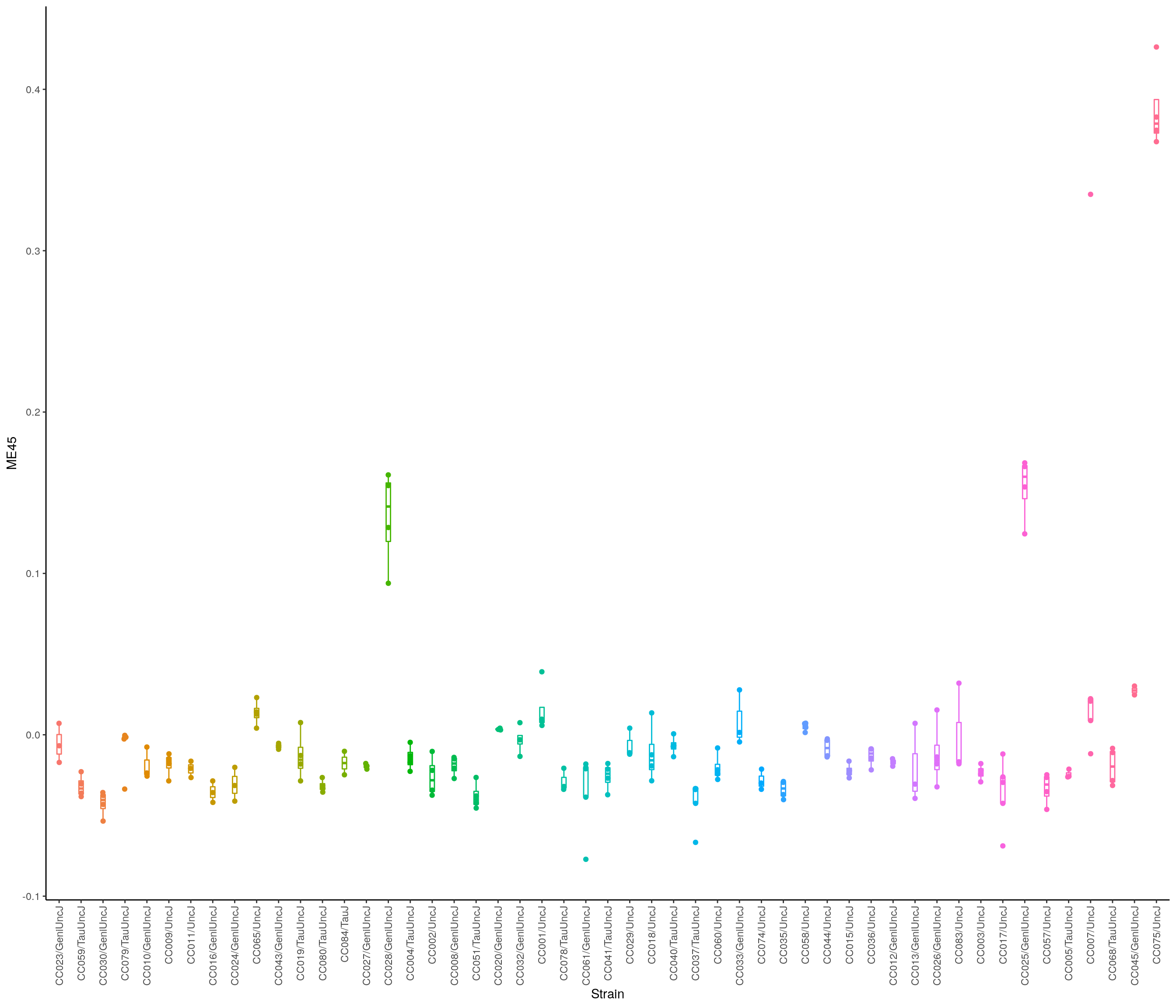
#hub genes
hubs = chooseTopHubInEachModule(expression, bwnet$colors)
hubs_df = data.frame(hubgene = hubs, mark_hub_gene_in_module = paste0("ME", names(hubs)))
#gene content
gene_module_key <- tibble::enframe(bwnet$colors, name = "gene", value = "module") %>%
# Let's add the `ME` part so its more clear what these numbers are and it matches elsewhere
dplyr::mutate(module = paste0("ME", module)) %>%
dplyr::left_join(genes, by = c("gene" = "ENSEMBL")) %>%
dplyr::left_join(hubs_df, by = c("gene" = "hubgene"))
#display stats_df
DT::datatable(gene_module_key,
filter = list(position = 'top', clear = FALSE),
extensions = 'Buttons',
options = list(dom = 'Blfrtip',
buttons = c('csv', 'excel'),
lengthMenu = list(c(10,25,50,-1),
c(10,25,50,"All")),
pageLength = 40,
scrollY = "300px",
scrollX = "40px"),
caption = htmltools::tags$caption(style = 'caption-side: top; text-align: left; color:black; font-size:200% ;',
'Module gene content'))Warning in instance$preRenderHook(instance): It seems your data is too big
for client-side DataTables. You may consider server-side processing: https://
rstudio.github.io/DT/server.htmlnGenes = ncol(expression)
nSamples = nrow(expression)
MEs0 <- moduleEigengenes(expression, gsub("ME", "", gene_module_key$module))$eigengenes
MEs <- orderMEs(MEs0)
corType = "pearson"
robustY = ifelse(corType=="pearson",T,F)
all.equal(rownames(MEs), (design.matrix.pheno[rownames(df[df$Tissue == "NTS",]),]$name))[1] TRUEmodCor = cor(MEs, design.matrix.pheno[rownames(df[df$Tissue == "NTS",]),][,colnames(design.matrix.pheno)[27:176]], use = "p")
modCor = modCor[,colSums(!is.na(modCor)) > 0]
modP = corPvalueStudent(modCor, nSamples)
modP = modP[,colSums(!is.na(modP)) > 0]
modCor_results <- as.data.frame(modCor)
modadjustP_results <- as.data.frame(modP) %>%
dplyr::mutate(across(.cols = everything(), ~p.adjust(.x, method = "fdr")))
#display modCor_results
DT::datatable(modCor_results,
filter = list(position = 'top', clear = FALSE),
extensions = 'Buttons',
options = list(dom = 'Blfrtip',
buttons = c('csv', 'excel'),
lengthMenu = list(c(10,25,50,-1),
c(10,25,50,"All")),
pageLength = 40,
scrollY = "300px",
scrollX = "40px"),
caption = htmltools::tags$caption(style = 'caption-side: top; text-align: left; color:black; font-size:200% ;',
'Module-phenotype correlation'))#display modadjustP_results
DT::datatable(modadjustP_results,
filter = list(position = 'top', clear = FALSE),
extensions = 'Buttons',
options = list(dom = 'Blfrtip',
buttons = c('csv', 'excel'),
lengthMenu = list(c(10,25,50,-1),
c(10,25,50,"All")),
pageLength = 40,
scrollY = "300px",
scrollX = "40px"),
caption = htmltools::tags$caption(style = 'caption-side: top; text-align: left; color:black; font-size:200% ;',
'Adjusted p values for module-phenotype correlation'))
sessionInfo()R version 4.0.3 (2020-10-10)
Platform: x86_64-pc-linux-gnu (64-bit)
Running under: Ubuntu 20.04.2 LTS
Matrix products: default
BLAS/LAPACK: /usr/lib/x86_64-linux-gnu/openblas-pthread/libopenblasp-r0.3.8.so
locale:
[1] LC_CTYPE=en_US.UTF-8 LC_NUMERIC=C
[3] LC_TIME=en_US.UTF-8 LC_COLLATE=en_US.UTF-8
[5] LC_MONETARY=en_US.UTF-8 LC_MESSAGES=C
[7] LC_PAPER=en_US.UTF-8 LC_NAME=C
[9] LC_ADDRESS=C LC_TELEPHONE=C
[11] LC_MEASUREMENT=en_US.UTF-8 LC_IDENTIFICATION=C
attached base packages:
[1] grid parallel stats4 stats graphics grDevices utils
[8] datasets methods base
other attached packages:
[1] WGCNA_1.69 fastcluster_1.1.25
[3] dynamicTreeCut_1.63-1 data.table_1.13.6
[5] ggplotify_0.0.5 cowplot_1.1.1
[7] enrichR_3.0 DT_0.17
[9] ggrepel_0.9.1 pheatmap_1.0.12
[11] DESeq2_1.30.1 SummarizedExperiment_1.20.0
[13] MatrixGenerics_1.2.1 matrixStats_0.58.0
[15] GenomicRanges_1.42.0 GenomeInfoDb_1.26.7
[17] RColorBrewer_1.1-2 org.Mm.eg.db_3.12.0
[19] AnnotationDbi_1.52.0 IRanges_2.24.1
[21] S4Vectors_0.28.1 Biobase_2.50.0
[23] BiocGenerics_0.36.1 gplots_3.1.1
[25] Glimma_2.0.0 edgeR_3.32.1
[27] limma_3.46.0 forcats_0.5.1
[29] dplyr_1.0.4 purrr_0.3.4
[31] readr_1.4.0 tidyr_1.1.2
[33] tibble_3.0.6 ggplot2_3.3.3
[35] tidyverse_1.3.0 stringr_1.4.0
[37] workflowr_1.6.2
loaded via a namespace (and not attached):
[1] readxl_1.3.1 backports_1.2.1 Hmisc_4.4-2
[4] splines_4.0.3 crosstalk_1.1.1 BiocParallel_1.24.1
[7] digest_0.6.27 foreach_1.5.1 htmltools_0.5.1.1
[10] GO.db_3.12.1 checkmate_2.0.0 magrittr_2.0.1
[13] memoise_2.0.0 cluster_2.1.1 doParallel_1.0.16
[16] annotate_1.68.0 modelr_0.1.8 jpeg_0.1-8.1
[19] colorspace_2.0-0 blob_1.2.1 rvest_0.3.6
[22] haven_2.3.1 xfun_0.21 crayon_1.4.1
[25] RCurl_1.98-1.2 jsonlite_1.7.2 genefilter_1.72.1
[28] impute_1.64.0 survival_3.2-7 iterators_1.0.13
[31] glue_1.4.2 polyclip_1.10-0 gtable_0.3.0
[34] zlibbioc_1.36.0 XVector_0.30.0 DelayedArray_0.16.3
[37] scales_1.1.1 DBI_1.1.1 Rcpp_1.0.6
[40] htmlTable_2.1.0 xtable_1.8-4 gridGraphics_0.5-1
[43] foreign_0.8-81 bit_4.0.4 preprocessCore_1.52.1
[46] Formula_1.2-4 htmlwidgets_1.5.3 httr_1.4.2
[49] ellipsis_0.3.1 farver_2.0.3 pkgconfig_2.0.3
[52] XML_3.99-0.5 nnet_7.3-15 dbplyr_2.1.0
[55] locfit_1.5-9.4 labeling_0.4.2 tidyselect_1.1.0
[58] rlang_1.0.2 later_1.1.0.1 munsell_0.5.0
[61] cellranger_1.1.0 tools_4.0.3 cachem_1.0.4
[64] cli_2.3.0 generics_0.1.0 RSQLite_2.2.3
[67] broom_0.7.4 evaluate_0.14 fastmap_1.1.0
[70] yaml_2.2.1 knitr_1.31 bit64_4.0.5
[73] fs_1.5.0 caTools_1.18.1 whisker_0.4
[76] xml2_1.3.2 compiler_4.0.3 rstudioapi_0.13
[79] curl_4.3 png_0.1-7 reprex_1.0.0
[82] tweenr_1.0.1 geneplotter_1.68.0 stringi_1.5.3
[85] highr_0.8 lattice_0.20-41 Matrix_1.3-2
[88] vctrs_0.3.6 pillar_1.4.7 lifecycle_1.0.0
[91] BiocManager_1.30.10 bitops_1.0-6 httpuv_1.5.5
[94] R6_2.5.0 latticeExtra_0.6-29 promises_1.2.0.1
[97] gridExtra_2.3 KernSmooth_2.23-18 codetools_0.2-18
[100] MASS_7.3-53.1 gtools_3.8.2 assertthat_0.2.1
[103] rprojroot_2.0.2 rjson_0.2.20 withr_2.4.1
[106] GenomeInfoDbData_1.2.4 hms_1.0.0 rpart_4.1-15
[109] rmarkdown_2.6 rvcheck_0.1.8 git2r_0.28.0
[112] ggforce_0.3.2 lubridate_1.7.9.2 base64enc_0.1-3 This R Markdown site was created with workflowr