PMCA
Hao He
2025-02-05
Last updated: 2025-02-05
Checks: 7 0
Knit directory: DO_Opioid/
This reproducible R Markdown analysis was created with workflowr (version 1.6.2). The Checks tab describes the reproducibility checks that were applied when the results were created. The Past versions tab lists the development history.
Great! Since the R Markdown file has been committed to the Git repository, you know the exact version of the code that produced these results.
Great job! The global environment was empty. Objects defined in the global environment can affect the analysis in your R Markdown file in unknown ways. For reproduciblity it’s best to always run the code in an empty environment.
The command set.seed(20200504) was run prior to running the code in the R Markdown file. Setting a seed ensures that any results that rely on randomness, e.g. subsampling or permutations, are reproducible.
Great job! Recording the operating system, R version, and package versions is critical for reproducibility.
Nice! There were no cached chunks for this analysis, so you can be confident that you successfully produced the results during this run.
Great job! Using relative paths to the files within your workflowr project makes it easier to run your code on other machines.
Great! You are using Git for version control. Tracking code development and connecting the code version to the results is critical for reproducibility.
The results in this page were generated with repository version 81f307d. See the Past versions tab to see a history of the changes made to the R Markdown and HTML files.
Note that you need to be careful to ensure that all relevant files for the analysis have been committed to Git prior to generating the results (you can use wflow_publish or wflow_git_commit). workflowr only checks the R Markdown file, but you know if there are other scripts or data files that it depends on. Below is the status of the Git repository when the results were generated:
Ignored files:
    Ignored:    .RData
    Ignored:    .Rhistory
    Ignored:    .Rproj.user/
    Ignored:    analysis/Picture1.png

Untracked files:
    Untracked:  analysis/BOT_NTS_modQTL.R
    Untracked:  analysis/BOT_NTS_modQTL.Rout
    Untracked:  analysis/BOT_modQTL.R
    Untracked:  analysis/BOT_modQTL.sh
    Untracked:  analysis/BOT_modQTL.stderr
    Untracked:  analysis/BOT_modQTL.stdout
    Untracked:  analysis/DDO_morphine1_second_set_69k.stdout
    Untracked:  analysis/DO_Fentanyl.R
    Untracked:  analysis/DO_Fentanyl.err
    Untracked:  analysis/DO_Fentanyl.out
    Untracked:  analysis/DO_Fentanyl.sh
    Untracked:  analysis/DO_Fentanyl_69k.R
    Untracked:  analysis/DO_Fentanyl_69k.err
    Untracked:  analysis/DO_Fentanyl_69k.out
    Untracked:  analysis/DO_Fentanyl_69k.sh
    Untracked:  analysis/DO_Fentanyl_Cohort2_GCTA_herit.R
    Untracked:  analysis/DO_Fentanyl_Cohort2_gemma.R
    Untracked:  analysis/DO_Fentanyl_Cohort2_mapping.R
    Untracked:  analysis/DO_Fentanyl_Cohort2_mapping.err
    Untracked:  analysis/DO_Fentanyl_Cohort2_mapping.out
    Untracked:  analysis/DO_Fentanyl_Cohort2_mapping.sh
    Untracked:  analysis/DO_Fentanyl_GCTA_herit.R
    Untracked:  analysis/DO_Fentanyl_alternate_metrics_69k.R
    Untracked:  analysis/DO_Fentanyl_alternate_metrics_69k.err
    Untracked:  analysis/DO_Fentanyl_alternate_metrics_69k.out
    Untracked:  analysis/DO_Fentanyl_alternate_metrics_69k.sh
    Untracked:  analysis/DO_Fentanyl_alternate_metrics_array.R
    Untracked:  analysis/DO_Fentanyl_alternate_metrics_array.err
    Untracked:  analysis/DO_Fentanyl_alternate_metrics_array.out
    Untracked:  analysis/DO_Fentanyl_alternate_metrics_array.sh
    Untracked:  analysis/DO_Fentanyl_array.R
    Untracked:  analysis/DO_Fentanyl_array.err
    Untracked:  analysis/DO_Fentanyl_array.out
    Untracked:  analysis/DO_Fentanyl_array.sh
    Untracked:  analysis/DO_Fentanyl_combining2Cohort_GCTA_herit.R
    Untracked:  analysis/DO_Fentanyl_combining2Cohort_gemma.R
    Untracked:  analysis/DO_Fentanyl_combining2Cohort_mapping.R
    Untracked:  analysis/DO_Fentanyl_combining2Cohort_mapping.err
    Untracked:  analysis/DO_Fentanyl_combining2Cohort_mapping.out
    Untracked:  analysis/DO_Fentanyl_combining2Cohort_mapping.sh
    Untracked:  analysis/DO_Fentanyl_combining2Cohort_mapping_CoxPH.R
    Untracked:  analysis/DO_Fentanyl_finalreport_to_plink.sh
    Untracked:  analysis/DO_Fentanyl_gemma.R
    Untracked:  analysis/DO_Fentanyl_gemma.err
    Untracked:  analysis/DO_Fentanyl_gemma.out
    Untracked:  analysis/DO_Fentanyl_gemma.sh
    Untracked:  analysis/DO_morphine1.R
    Untracked:  analysis/DO_morphine1.Rout
    Untracked:  analysis/DO_morphine1.sh
    Untracked:  analysis/DO_morphine1.stderr
    Untracked:  analysis/DO_morphine1.stdout
    Untracked:  analysis/DO_morphine1_SNP.R
    Untracked:  analysis/DO_morphine1_SNP.Rout
    Untracked:  analysis/DO_morphine1_SNP.sh
    Untracked:  analysis/DO_morphine1_SNP.stderr
    Untracked:  analysis/DO_morphine1_SNP.stdout
    Untracked:  analysis/DO_morphine1_combined.R
    Untracked:  analysis/DO_morphine1_combined.Rout
    Untracked:  analysis/DO_morphine1_combined.sh
    Untracked:  analysis/DO_morphine1_combined.stderr
    Untracked:  analysis/DO_morphine1_combined.stdout
    Untracked:  analysis/DO_morphine1_combined_69k.R
    Untracked:  analysis/DO_morphine1_combined_69k.Rout
    Untracked:  analysis/DO_morphine1_combined_69k.sh
    Untracked:  analysis/DO_morphine1_combined_69k.stderr
    Untracked:  analysis/DO_morphine1_combined_69k.stdout
    Untracked:  analysis/DO_morphine1_combined_69k_m2.R
    Untracked:  analysis/DO_morphine1_combined_69k_m2.Rout
    Untracked:  analysis/DO_morphine1_combined_69k_m2.sh
    Untracked:  analysis/DO_morphine1_combined_69k_m2.stderr
    Untracked:  analysis/DO_morphine1_combined_69k_m2.stdout
    Untracked:  analysis/DO_morphine1_combined_weight_DOB.R
    Untracked:  analysis/DO_morphine1_combined_weight_DOB.Rout
    Untracked:  analysis/DO_morphine1_combined_weight_DOB.err
    Untracked:  analysis/DO_morphine1_combined_weight_DOB.out
    Untracked:  analysis/DO_morphine1_combined_weight_DOB.sh
    Untracked:  analysis/DO_morphine1_combined_weight_DOB.stderr
    Untracked:  analysis/DO_morphine1_combined_weight_DOB.stdout
    Untracked:  analysis/DO_morphine1_combined_weight_age.R
    Untracked:  analysis/DO_morphine1_combined_weight_age.err
    Untracked:  analysis/DO_morphine1_combined_weight_age.out
    Untracked:  analysis/DO_morphine1_combined_weight_age.sh
    Untracked:  analysis/DO_morphine1_combined_weight_age_GAMMT.R
    Untracked:  analysis/DO_morphine1_combined_weight_age_GAMMT.err
    Untracked:  analysis/DO_morphine1_combined_weight_age_GAMMT.out
    Untracked:  analysis/DO_morphine1_combined_weight_age_GAMMT.sh
    Untracked:  analysis/DO_morphine1_combined_weight_age_GAMMT_chr19.R
    Untracked:  analysis/DO_morphine1_combined_weight_age_GAMMT_chr19.err
    Untracked:  analysis/DO_morphine1_combined_weight_age_GAMMT_chr19.out
    Untracked:  analysis/DO_morphine1_combined_weight_age_GAMMT_chr19.sh
    Untracked:  analysis/DO_morphine1_cph.R
    Untracked:  analysis/DO_morphine1_cph.Rout
    Untracked:  analysis/DO_morphine1_cph.sh
    Untracked:  analysis/DO_morphine1_second_set.R
    Untracked:  analysis/DO_morphine1_second_set.Rout
    Untracked:  analysis/DO_morphine1_second_set.sh
    Untracked:  analysis/DO_morphine1_second_set.stderr
    Untracked:  analysis/DO_morphine1_second_set.stdout
    Untracked:  analysis/DO_morphine1_second_set_69k.R
    Untracked:  analysis/DO_morphine1_second_set_69k.Rout
    Untracked:  analysis/DO_morphine1_second_set_69k.sh
    Untracked:  analysis/DO_morphine1_second_set_69k.stderr
    Untracked:  analysis/DO_morphine1_second_set_SNP.R
    Untracked:  analysis/DO_morphine1_second_set_SNP.Rout
    Untracked:  analysis/DO_morphine1_second_set_SNP.sh
    Untracked:  analysis/DO_morphine1_second_set_SNP.stderr
    Untracked:  analysis/DO_morphine1_second_set_SNP.stdout
    Untracked:  analysis/DO_morphine1_second_set_weight_DOB.R
    Untracked:  analysis/DO_morphine1_second_set_weight_DOB.Rout
    Untracked:  analysis/DO_morphine1_second_set_weight_DOB.err
    Untracked:  analysis/DO_morphine1_second_set_weight_DOB.out
    Untracked:  analysis/DO_morphine1_second_set_weight_DOB.sh
    Untracked:  analysis/DO_morphine1_second_set_weight_DOB.stderr
    Untracked:  analysis/DO_morphine1_second_set_weight_DOB.stdout
    Untracked:  analysis/DO_morphine1_second_set_weight_age.R
    Untracked:  analysis/DO_morphine1_second_set_weight_age.Rout
    Untracked:  analysis/DO_morphine1_second_set_weight_age.err
    Untracked:  analysis/DO_morphine1_second_set_weight_age.out
    Untracked:  analysis/DO_morphine1_second_set_weight_age.sh
    Untracked:  analysis/DO_morphine1_second_set_weight_age.stderr
    Untracked:  analysis/DO_morphine1_second_set_weight_age.stdout
    Untracked:  analysis/DO_morphine1_weight_DOB.R
    Untracked:  analysis/DO_morphine1_weight_DOB.sh
    Untracked:  analysis/DO_morphine1_weight_age.R
    Untracked:  analysis/DO_morphine1_weight_age.sh
    Untracked:  analysis/DO_morphine_gemma.R
    Untracked:  analysis/DO_morphine_gemma.err
    Untracked:  analysis/DO_morphine_gemma.out
    Untracked:  analysis/DO_morphine_gemma.sh
    Untracked:  analysis/DO_morphine_gemma_firstmin.R
    Untracked:  analysis/DO_morphine_gemma_firstmin.err
    Untracked:  analysis/DO_morphine_gemma_firstmin.out
    Untracked:  analysis/DO_morphine_gemma_firstmin.sh
    Untracked:  analysis/DO_morphine_gemma_withpermu.R
    Untracked:  analysis/DO_morphine_gemma_withpermu.err
    Untracked:  analysis/DO_morphine_gemma_withpermu.out
    Untracked:  analysis/DO_morphine_gemma_withpermu.sh
    Untracked:  analysis/DO_morphine_gemma_withpermu_firstbatch_min.depression.R
    Untracked:  analysis/DO_morphine_gemma_withpermu_firstbatch_min.depression.err
    Untracked:  analysis/DO_morphine_gemma_withpermu_firstbatch_min.depression.out
    Untracked:  analysis/DO_morphine_gemma_withpermu_firstbatch_min.depression.sh
    Untracked:  analysis/Lisa_Tarantino_Interval_needs_mvar_annotation.R
    Untracked:  analysis/NTS_modQTL.R
    Untracked:  analysis/NTS_modQTL.sh
    Untracked:  analysis/NTS_modQTL.stderr
    Untracked:  analysis/NTS_modQTL.stdout
    Untracked:  analysis/Plot_DO_morphine1_SNP.R
    Untracked:  analysis/Plot_DO_morphine1_SNP.Rout
    Untracked:  analysis/Plot_DO_morphine1_SNP.sh
    Untracked:  analysis/Plot_DO_morphine1_SNP.stderr
    Untracked:  analysis/Plot_DO_morphine1_SNP.stdout
    Untracked:  analysis/Plot_DO_morphine1_second_set_SNP.R
    Untracked:  analysis/Plot_DO_morphine1_second_set_SNP.Rout
    Untracked:  analysis/Plot_DO_morphine1_second_set_SNP.sh
    Untracked:  analysis/Plot_DO_morphine1_second_set_SNP.stderr
    Untracked:  analysis/Plot_DO_morphine1_second_set_SNP.stdout
    Untracked:  analysis/cecum_meQTL.R
    Untracked:  analysis/cecum_meQTL.sh
    Untracked:  analysis/cecum_meQTL.stderr
    Untracked:  analysis/cecum_meQTL.stdout
    Untracked:  analysis/combined_modQTL.R
    Untracked:  analysis/combined_modQTL.sh
    Untracked:  analysis/combined_modQTL.stderr
    Untracked:  analysis/combined_modQTL.stdout
    Untracked:  analysis/download_GSE100356_sra.sh
    Untracked:  analysis/fentanyl_2cohorts_coxph.R
    Untracked:  analysis/fentanyl_2cohorts_coxph.err
    Untracked:  analysis/fentanyl_2cohorts_coxph.out
    Untracked:  analysis/fentanyl_2cohorts_coxph.sh
    Untracked:  analysis/fentanyl_scanone.cph.R
    Untracked:  analysis/fentanyl_scanone.cph.err
    Untracked:  analysis/fentanyl_scanone.cph.out
    Untracked:  analysis/fentanyl_scanone.cph.sh
    Untracked:  analysis/geo_rnaseq.R
    Untracked:  analysis/heritability_first_second_batch.R
    Untracked:  analysis/morphine_fentanyl_survival_time.R
    Untracked:  analysis/mvar_annotation.R
    Untracked:  analysis/mvar_annotation.Rout
    Untracked:  analysis/nf-rnaseq-b6.R
    Untracked:  analysis/pipeline_qtl2.R
    Untracked:  analysis/plot_fentanyl_2cohorts_coxph.R
    Untracked:  analysis/scripts/
    Untracked:  analysis/striatum_meQTL.R
    Untracked:  analysis/striatum_meQTL.sh
    Untracked:  analysis/striatum_meQTL.stderr
    Untracked:  analysis/striatum_meQTL.stdout
    Untracked:  analysis/tibmr.R
    Untracked:  analysis/timbr_demo.R
    Untracked:  analysis/upset.R
    Untracked:  analysis/workflow_proc.R
    Untracked:  analysis/workflow_proc.sh
    Untracked:  analysis/workflow_proc.stderr
    Untracked:  analysis/workflow_proc.stdout
    Untracked:  analysis/x.R
    Untracked:  analysis/~.sh
    Untracked:  check_do.R
    Untracked:  code/PLINKtoCSVR.R
    Untracked:  code/additive_scan1_HPC.R
    Untracked:  code/cfw/
    Untracked:  code/combine_adjacency_matrices.R
    Untracked:  code/extract_edgelist_from_adjacency.R
    Untracked:  code/fit_lm_function.R
    Untracked:  code/fit_model.R
    Untracked:  code/gather_scan1_chunks.R
    Untracked:  code/gemma_plot.R
    Untracked:  code/get_edgelist.R
    Untracked:  code/new1.R
    Untracked:  code/new2.R
    Untracked:  code/process.sanger.snp.R
    Untracked:  code/reconst_utils.R
    Untracked:  code/scan1_permutation_HPC.R
    Untracked:  code/scan1_pvalue_ciseqtl.HPC.R
    Untracked:  code/utils.R
    Untracked:  complete_traits_20241212.csv
    Untracked:  data/69k_grid_pgmap.RData
    Untracked:  data/BOT_NTS_rnaseq_results/
    Untracked:  data/CC_SARS-1/
    Untracked:  data/CC_SARS-2/
    Untracked:  data/Composite Post Kevins Program Group 2 Fentanyl Prepped for Hao.xlsx
    Untracked:  data/Current CHr 11 Complete Query.csv
    Untracked:  data/DO_WBP_Data_JAB_to_map.xlsx
    Untracked:  data/DO_new_traits/
    Untracked:  data/Data_repository_Bubier/
    Untracked:  data/Fentanyl_alternate_metrics.xlsx
    Untracked:  data/FinalReport/
    Untracked:  data/GM/
    Untracked:  data/GM_covar.csv
    Untracked:  data/GM_covar_07092018_morphine.csv
    Untracked:  data/Jackson_Lab_Bubier_MURGIGV01/
    Untracked:  data/Lisa Tarantino Interval needs mvar.xlsx
    Untracked:  data/Lisa_Tarantino_Interval_needs_mvar_annotation.csv
    Untracked:  data/MPD_Upload_October.csv
    Untracked:  data/MPD_Upload_October_updated_sex.csv
    Untracked:  data/Master Fentanyl DO Study Sheet.xlsx
    Untracked:  data/MasterMorphine Second Set DO w DOB2.xlsx
    Untracked:  data/MasterMorphine Second Set DO.xlsx
    Untracked:  data/Morphine CC DO mice Updated with Published inbred strains.csv
    Untracked:  data/Morphine_CC_DO_mice_Updated_with_Published_inbred_strains.csv
    Untracked:  data/cc_variants.sqlite
    Untracked:  data/combined/
    Untracked:  data/fentanyl/
    Untracked:  data/fentanyl2/
    Untracked:  data/fentanyl_1_2/
    Untracked:  data/fentanyl_2cohorts_coxph_data.Rdata
    Untracked:  data/first/
    Untracked:  data/founder_geno.csv
    Untracked:  data/genetic_map.csv
    Untracked:  data/gm.json
    Untracked:  data/gwas.sh
    Untracked:  data/marker_grid_0.02cM_plus.txt
    Untracked:  data/metabolomics_mouse_fecal/
    Untracked:  data/mouse_genes_mgi.sqlite
    Untracked:  data/pheno.csv
    Untracked:  data/pheno_qtl2.csv
    Untracked:  data/pheno_qtl2_07092018_morphine.csv
    Untracked:  data/pheno_qtl2_w_dob.csv
    Untracked:  data/physical_map.csv
    Untracked:  data/rnaseq/
    Untracked:  data/sample_geno.csv
    Untracked:  data/second/
    Untracked:  figure/
    Untracked:  glimma-plots/
    Untracked:  output/DO_Fentanyl_Cohort2_MinDepressionRR_coefplot.pdf
    Untracked:  output/DO_Fentanyl_Cohort2_MinDepressionRR_coefplot_blup.pdf
    Untracked:  output/DO_Fentanyl_Cohort2_RRDepressionRateHrSLOPE_coefplot.pdf
    Untracked:  output/DO_Fentanyl_Cohort2_RRRecoveryRateHrSLOPE_coefplot.pdf
    Untracked:  output/DO_Fentanyl_Cohort2_RRRecoveryRateHrSLOPE_coefplot_blup.pdf
    Untracked:  output/DO_Fentanyl_Cohort2_StartofRecoveryHr_coefplot.pdf
    Untracked:  output/DO_Fentanyl_Cohort2_StartofRecoveryHr_coefplot_blup.pdf
    Untracked:  output/DO_Fentanyl_Cohort2_Statusbin_coefplot.pdf
    Untracked:  output/DO_Fentanyl_Cohort2_Statusbin_coefplot_blup.pdf
    Untracked:  output/DO_Fentanyl_Cohort2_SteadyStateDepressionDurationHrINTERVAL_coefplot.pdf
    Untracked:  output/DO_Fentanyl_Cohort2_TimetoDead(Hr)_coefplot.pdf
    Untracked:  output/DO_Fentanyl_Cohort2_TimetoDeadHr_coefplot.pdf
    Untracked:  output/DO_Fentanyl_Cohort2_TimetoDeadHr_coefplot_blup.pdf
    Untracked:  output/DO_Fentanyl_Cohort2_TimetoProjectedRecoveryHr_coefplot.pdf
    Untracked:  output/DO_Fentanyl_Cohort2_TimetoProjectedRecoveryHr_coefplot_blup.pdf
    Untracked:  output/DO_Fentanyl_Cohort2_TimetoSteadyRRDepression(Hr)_coefplot.pdf
    Untracked:  output/DO_Fentanyl_Cohort2_TimetoSteadyRRDepressionHr_coefplot.pdf
    Untracked:  output/DO_Fentanyl_Cohort2_TimetoSteadyRRDepressionHr_coefplot_blup.pdf
    Untracked:  output/DO_Fentanyl_Cohort2_TimetoThresholdRecoveryHr_coefplot.pdf
    Untracked:  output/DO_Fentanyl_Cohort2_TimetoThresholdRecoveryHr_coefplot_blup.pdf
    Untracked:  output/DO_morphine_Min.depression.png
    Untracked:  output/DO_morphine_Min.depression22222_violin_chr5.pdf
    Untracked:  output/DO_morphine_Min.depression_coefplot.pdf
    Untracked:  output/DO_morphine_Min.depression_coefplot_blup.pdf
    Untracked:  output/DO_morphine_Min.depression_coefplot_blup_chr5.png
    Untracked:  output/DO_morphine_Min.depression_coefplot_blup_chrX.png
    Untracked:  output/DO_morphine_Min.depression_coefplot_chr5.png
    Untracked:  output/DO_morphine_Min.depression_coefplot_chrX.png
    Untracked:  output/DO_morphine_Min.depression_peak_genes_chr5.png
    Untracked:  output/DO_morphine_Min.depression_violin_chr5.png
    Untracked:  output/DO_morphine_Recovery.Time.png
    Untracked:  output/DO_morphine_Recovery.Time_coefplot.pdf
    Untracked:  output/DO_morphine_Recovery.Time_coefplot_blup.pdf
    Untracked:  output/DO_morphine_Recovery.Time_coefplot_blup_chr11.png
    Untracked:  output/DO_morphine_Recovery.Time_coefplot_blup_chr4.png
    Untracked:  output/DO_morphine_Recovery.Time_coefplot_blup_chr7.png
    Untracked:  output/DO_morphine_Recovery.Time_coefplot_blup_chr9.png
    Untracked:  output/DO_morphine_Recovery.Time_coefplot_chr11.png
    Untracked:  output/DO_morphine_Recovery.Time_coefplot_chr4.png
    Untracked:  output/DO_morphine_Recovery.Time_coefplot_chr7.png
    Untracked:  output/DO_morphine_Recovery.Time_coefplot_chr9.png
    Untracked:  output/DO_morphine_Status_bin.png
    Untracked:  output/DO_morphine_Status_bin_coefplot.pdf
    Untracked:  output/DO_morphine_Status_bin_coefplot_blup.pdf
    Untracked:  output/DO_morphine_Survival.Time.png
    Untracked:  output/DO_morphine_Survival.Time_coefplot.pdf
    Untracked:  output/DO_morphine_Survival.Time_coefplot_blup.pdf
    Untracked:  output/DO_morphine_Survival.Time_coefplot_blup_chr17.png
    Untracked:  output/DO_morphine_Survival.Time_coefplot_blup_chr8.png
    Untracked:  output/DO_morphine_Survival.Time_coefplot_chr17.png
    Untracked:  output/DO_morphine_Survival.Time_coefplot_chr8.png
    Untracked:  output/DO_morphine_combine_batch_peak_violin.pdf
    Untracked:  output/DO_morphine_combined_69k_m2_Min.depression.png
    Untracked:  output/DO_morphine_combined_69k_m2_Min.depression_coefplot.pdf
    Untracked:  output/DO_morphine_combined_69k_m2_Min.depression_coefplot_blup.pdf
    Untracked:  output/DO_morphine_combined_69k_m2_Recovery.Time.png
    Untracked:  output/DO_morphine_combined_69k_m2_Recovery.Time_coefplot.pdf
    Untracked:  output/DO_morphine_combined_69k_m2_Recovery.Time_coefplot_blup.pdf
    Untracked:  output/DO_morphine_combined_69k_m2_Status_bin.png
    Untracked:  output/DO_morphine_combined_69k_m2_Status_bin_coefplot.pdf
    Untracked:  output/DO_morphine_combined_69k_m2_Status_bin_coefplot_blup.pdf
    Untracked:  output/DO_morphine_combined_69k_m2_Survival.Time.png
    Untracked:  output/DO_morphine_combined_69k_m2_Survival.Time_coefplot.pdf
    Untracked:  output/DO_morphine_combined_69k_m2_Survival.Time_coefplot_blup.pdf
    Untracked:  output/DO_morphine_coxph_24hrs_kinship_QTL.png
    Untracked:  output/DO_morphine_cphout.RData
    Untracked:  output/DO_morphine_first_batch_peak_in_second_batch_violin.pdf
    Untracked:  output/DO_morphine_first_batch_peak_in_second_batch_violin_sidebyside.pdf
    Untracked:  output/DO_morphine_first_batch_peak_violin.pdf
    Untracked:  output/DO_morphine_operm.cph.RData
    Untracked:  output/DO_morphine_second_batch_on_first_batch_peak_violin.pdf
    Untracked:  output/DO_morphine_second_batch_peak_ch6surv_on_first_batchviolin.pdf
    Untracked:  output/DO_morphine_second_batch_peak_ch6surv_on_first_batchviolin2.pdf
    Untracked:  output/DO_morphine_second_batch_peak_in_first_batch_violin.pdf
    Untracked:  output/DO_morphine_second_batch_peak_in_first_batch_violin_sidebyside.pdf
    Untracked:  output/DO_morphine_second_batch_peak_violin.pdf
    Untracked:  output/DO_morphine_secondbatch_69k_Min.depression.png
    Untracked:  output/DO_morphine_secondbatch_69k_Min.depression_coefplot.pdf
    Untracked:  output/DO_morphine_secondbatch_69k_Min.depression_coefplot_blup.pdf
    Untracked:  output/DO_morphine_secondbatch_69k_Recovery.Time.png
    Untracked:  output/DO_morphine_secondbatch_69k_Recovery.Time_coefplot.pdf
    Untracked:  output/DO_morphine_secondbatch_69k_Recovery.Time_coefplot_blup.pdf
    Untracked:  output/DO_morphine_secondbatch_69k_Status_bin.png
    Untracked:  output/DO_morphine_secondbatch_69k_Status_bin_coefplot.pdf
    Untracked:  output/DO_morphine_secondbatch_69k_Status_bin_coefplot_blup.pdf
    Untracked:  output/DO_morphine_secondbatch_69k_Survival.Time.png
    Untracked:  output/DO_morphine_secondbatch_69k_Survival.Time_coefplot.pdf
    Untracked:  output/DO_morphine_secondbatch_69k_Survival.Time_coefplot_blup.pdf
    Untracked:  output/DO_morphine_secondbatch_Min.depression.png
    Untracked:  output/DO_morphine_secondbatch_Min.depression_coefplot.pdf
    Untracked:  output/DO_morphine_secondbatch_Min.depression_coefplot_blup.pdf
    Untracked:  output/DO_morphine_secondbatch_Recovery.Time.png
    Untracked:  output/DO_morphine_secondbatch_Recovery.Time_coefplot.pdf
    Untracked:  output/DO_morphine_secondbatch_Recovery.Time_coefplot_blup.pdf
    Untracked:  output/DO_morphine_secondbatch_Status_bin.png
    Untracked:  output/DO_morphine_secondbatch_Status_bin_coefplot.pdf
    Untracked:  output/DO_morphine_secondbatch_Status_bin_coefplot_blup.pdf
    Untracked:  output/DO_morphine_secondbatch_Survival.Time.png
    Untracked:  output/DO_morphine_secondbatch_Survival.Time_coefplot.pdf
    Untracked:  output/DO_morphine_secondbatch_Survival.Time_coefplot_blup.pdf
    Untracked:  output/Fentanyl/
    Untracked:  output/KPNA3.pdf
    Untracked:  output/PMCA/
    Untracked:  output/SSC4D.pdf
    Untracked:  output/TIMBR.test.RData
    Untracked:  output/apr_69kchr_combined.RData
    Untracked:  output/apr_69kchr_k_loco_combined.rds
    Untracked:  output/apr_69kchr_second_set.RData
    Untracked:  output/combine_batch_variation.RData
    Untracked:  output/combined_gm.RData
    Untracked:  output/combined_gm.k_loco.rds
    Untracked:  output/combined_gm.k_overall.rds
    Untracked:  output/combined_gm.probs_8state.rds
    Untracked:  output/coxph/
    Untracked:  output/do.morphine.RData
    Untracked:  output/do.morphine.k_loco.rds
    Untracked:  output/do.morphine.probs_36state.rds
    Untracked:  output/do.morphine.probs_8state.rds
    Untracked:  output/do_Fentanyl_combine2cohort_MeanDepressionBR_coefplot.pdf
    Untracked:  output/do_Fentanyl_combine2cohort_MeanDepressionBR_coefplot_blup.pdf
    Untracked:  output/do_Fentanyl_combine2cohort_MinDepressionBR_coefplot.pdf
    Untracked:  output/do_Fentanyl_combine2cohort_MinDepressionBR_coefplot_blup.pdf
    Untracked:  output/do_Fentanyl_combine2cohort_MinDepressionRR_coefplot.pdf
    Untracked:  output/do_Fentanyl_combine2cohort_MinDepressionRR_coefplot_blup.pdf
    Untracked:  output/do_Fentanyl_combine2cohort_RRRecoveryRateHr_coefplot.pdf
    Untracked:  output/do_Fentanyl_combine2cohort_RRRecoveryRateHr_coefplot_blup.pdf
    Untracked:  output/do_Fentanyl_combine2cohort_StartofRecoveryHr_coefplot.pdf
    Untracked:  output/do_Fentanyl_combine2cohort_StartofRecoveryHr_coefplot_blup.pdf
    Untracked:  output/do_Fentanyl_combine2cohort_Statusbin_coefplot.pdf
    Untracked:  output/do_Fentanyl_combine2cohort_Statusbin_coefplot_blup.pdf
    Untracked:  output/do_Fentanyl_combine2cohort_SteadyStateDepressionDurationHr_coefplot.pdf
    Untracked:  output/do_Fentanyl_combine2cohort_SteadyStateDepressionDurationHr_coefplot_blup.pdf
    Untracked:  output/do_Fentanyl_combine2cohort_SurvivalTime_coefplot.pdf
    Untracked:  output/do_Fentanyl_combine2cohort_SurvivalTime_coefplot_blup.pdf
    Untracked:  output/do_Fentanyl_combine2cohort_TimetoDeadHr_coefplot.pdf
    Untracked:  output/do_Fentanyl_combine2cohort_TimetoDeadHr_coefplot_blup.pdf
    Untracked:  output/do_Fentanyl_combine2cohort_TimetoMostlyDeadHr_coefplot.pdf
    Untracked:  output/do_Fentanyl_combine2cohort_TimetoMostlyDeadHr_coefplot_blup.pdf
    Untracked:  output/do_Fentanyl_combine2cohort_TimetoProjectedRecoveryHr_coefplot.pdf
    Untracked:  output/do_Fentanyl_combine2cohort_TimetoProjectedRecoveryHr_coefplot_blup.pdf
    Untracked:  output/do_Fentanyl_combine2cohort_TimetoRecoveryHr_coefplot.pdf
    Untracked:  output/do_Fentanyl_combine2cohort_TimetoRecoveryHr_coefplot_blup.pdf
    Untracked:  output/first_batch_variation.RData
    Untracked:  output/first_second_survival_peak_chr.xlsx
    Untracked:  output/hsq_1_first_batch_herit_qtl2.RData
    Untracked:  output/hsq_2_second_batch_herit_qtl2.RData
    Untracked:  output/meta.csv
    Untracked:  output/morphine_fentanyl_survival_time.pdf
    Untracked:  output/old_temp/
    Untracked:  output/out_1_operm.RData
    Untracked:  output/pr_69kchr_combined.RData
    Untracked:  output/pr_69kchr_second_set.RData
    Untracked:  output/qtl.morphine.69k.out.combined.RData
    Untracked:  output/qtl.morphine.69k.out.combined_m2.RData
    Untracked:  output/qtl.morphine.69k.out.second_set.RData
    Untracked:  output/qtl.morphine.operm.RData
    Untracked:  output/qtl.morphine.out.RData
    Untracked:  output/qtl.morphine.out.combined_gm.RData
    Untracked:  output/qtl.morphine.out.combined_gm.female.RData
    Untracked:  output/qtl.morphine.out.combined_gm.male.RData
    Untracked:  output/qtl.morphine.out.combined_weight_DOB.RData
    Untracked:  output/qtl.morphine.out.combined_weight_age.RData
    Untracked:  output/qtl.morphine.out.female.RData
    Untracked:  output/qtl.morphine.out.male.RData
    Untracked:  output/qtl.morphine.out.second_set.RData
    Untracked:  output/qtl.morphine.out.second_set.female.RData
    Untracked:  output/qtl.morphine.out.second_set.male.RData
    Untracked:  output/qtl.morphine.out.second_set.weight_DOB.RData
    Untracked:  output/qtl.morphine.out.second_set.weight_age.RData
    Untracked:  output/qtl.morphine.out.weight_DOB.RData
    Untracked:  output/qtl.morphine.out.weight_age.RData
    Untracked:  output/qtl.morphine1.snpout.RData
    Untracked:  output/qtl.morphine2.snpout.RData
    Untracked:  output/sample_all_infor.csv
    Untracked:  output/sample_all_infor.txt
    Untracked:  output/second_batch_pheno.csv
    Untracked:  output/second_batch_variation.RData
    Untracked:  output/second_set_apr_69kchr_k_loco.rds
    Untracked:  output/second_set_gm.RData
    Untracked:  output/second_set_gm.k_loco.rds
    Untracked:  output/second_set_gm.probs_36state.rds
    Untracked:  output/second_set_gm.probs_8state.rds
    Untracked:  output/topSNP_chr5_mindepression.csv
    Untracked:  output/zoompeak_Min.depression_9.pdf
    Untracked:  output/zoompeak_Recovery.Time_16.pdf
    Untracked:  output/zoompeak_Status_bin_11.pdf
    Untracked:  output/zoompeak_Survival.Time_1.pdf
    Untracked:  output/zoompeak_fentanyl_Survival.Time_2.pdf
    Untracked:  sra-tools_v2.10.7.sif

Unstaged changes:
    Modified:   .gitignore
    Modified:   _workflowr.yml
    Deleted:    analysis/CC_SARS-2.Rmd
    Modified:   analysis/CC_SARS.Rmd
    Modified:   analysis/DEG_analysis_BOT_vs_NTS.Rmd
    Modified:   analysis/marker_violin.Rmd
    Modified:   output/CC_SARS_Chr16_QTL_interval.pdf
    Modified:   output/CC_SARS_Chr16_plotGeno.pdf
    Modified:   output/CC_SARS_Chr16_plotGeno.png
Note that any generated files, e.g. HTML, png, CSS, etc., are not included in this status report because it is ok for generated content to have uncommitted changes.
These are the previous versions of the repository in which changes were made to the R Markdown (analysis/PMCA.Rmd) and HTML (docs/PMCA.html) files. If you’ve configured a remote Git repository (see ?wflow_git_remote), click on the hyperlinks in the table below to view the files as they were in that past version.
| File | Version | Author | Date | Message |
|---|---|---|---|---|
| Rmd | 81f307d | xhyuo | 2025-02-05 | PMCA sankey |
| html | 3724eb2 | xhyuo | 2025-01-16 | Build site. |
| Rmd | 042fa3e | xhyuo | 2025-01-16 | PMCA summary font |
| html | f7325c7 | xhyuo | 2025-01-15 | Build site. |
| Rmd | 3ccb2ad | xhyuo | 2025-01-15 | PMCA summary |
| html | 3577bf9 | xhyuo | 2025-01-08 | Build site. |
| Rmd | b93684b | xhyuo | 2025-01-08 | PMCA |
Last update: 2025-02-05
loading libraries
library(ComplexHeatmap)
library(tidyverse)
library(qtl2)
#devtools::install_github("robyn-ball/PMCA")
library(PMCA)
library(WGCNA)
library(circlize)
library(Hmisc)
library(PMCA)
library(RColorBrewer)
library(gplots)
library(biomaRt)
library(igraph)
library(networkD3)
source("code/utils.R")
source("code/get_edgelist.R")
source("code/combine_adjacency_matrices.R")
source("code/extract_edgelist_from_adjacency.R")
source("code/fit_lm_function.R")
# Test passed 😀
# Test passed 🎉
# Test passed 🎊
00 Upset plot
#load striatum expression data and WGCNA
striatum = readRDS("data/Data_repository_Bubier/striatum_expression/dataset.CSNA_DO_Striatum.v3.Rds")
stri_exp = striatum$data #it's 368 X 17248 matrix
#load cecum expression data
load("data/Data_repository_Bubier/cecum_expression/qtlviewer_DO_Cecum_416_06302020.RData")
cecum_exp = dataset.DO_Cecum_416$data #it's 267 X 15125 matrix
#load Novelty data
load("/projects/csna/csna_workflow/data/Jackson_Lab_13_batches/gm_13batches_newid_qc.RData")
#load cecal microbiome data
cecal_microb <- read.csv("data/Data_repository_Bubier/microbes/cecum_sq_genus_level_counts.csv", header = TRUE)
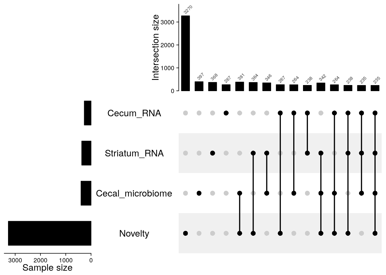
# Upset plot----------------------------------------------------------------
lt = list(Striatum_RNA = rownames(stri_exp),
Cecum_RNA = rownames(cecum_exp),
Novelty = ind_ids(gm_after_qc),
Cecal_microbiome = as.character(cecal_microb$X))
m = make_comb_mat(lt, mode = "intersect")
ss = set_size(m)
cs = comb_size(m)
ht = UpSet(m,
set_order = order(ss),
comb_order = order(comb_degree(m), -cs),
top_annotation = HeatmapAnnotation(
"Intersection size" = anno_barplot(cs,
ylim = c(0, max(cs)*1.1),
border = FALSE,
gp = gpar(fill = "black"),
height = unit(4, "cm")
),
annotation_name_side = "left",
annotation_name_rot = 90),
left_annotation = rowAnnotation(
"Sample size" = anno_barplot(-ss,
baseline = 0,
axis_param = list(
at = c(0, -1000, -2000, -3000, -4000),
labels = c(0, 1000, 2000, 3000, 4000),
labels_rot = 0),
border = FALSE,
gp = gpar(fill = "black"),
width = unit(4, "cm")
),
set_name = anno_text(set_name(m),
location = 0.5,
just = "center",
width = max_text_width(set_name(m)) + unit(4, "mm"))
),
right_annotation = NULL,
show_row_names = FALSE)
ht = draw(ht)
od = column_order(ht)
decorate_annotation("Intersection size", {
grid.text(cs[od], x = seq_along(cs), y = unit(cs[od], "native") + unit(2, "pt"),
default.units = "native", just = c("left", "bottom"),
gp = gpar(fontsize = 6, col = "#404040"), rot = 45)
})
| Version | Author | Date |
|---|---|---|
| 3577bf9 | xhyuo | 2025-01-08 |
01 Predisposing behaviors (data object: mat_predisposing_behaviors)
#Process HB phenotype data -----------------------------------------------------------------------
#select Total.Entries as entries_total_HB_do for HB Count of Total Nose Pokes in HB_raw_07012020.csv
DO.HB <- read.csv("/projects/csna/csna_workflow/data/pheno/HB_raw_07012020.csv", header = TRUE) %>%
  dplyr::select(Mouse.ID, Sex, entries_total_HB_do = Total.Entries)

#Process SENS_COCA phenotype data -----------------------------------------------------------------------
# D12_D2    dist_d12_d2_cocaine_do  COCA Conditioned Activation
# D11_D3    dist_d11_d3_cocaine_do  COCA Day 11 - Day 3
# D19_D11   dist_d19_d11_cocaine_do COCA Expression
# D3_D2   dist_d3_d2_cocaine_do   COCA Initial Sensitivity
# D5_D3   dist_d5_d3_cocaine_do   COCA Initial Sensitization
DO.SENS.COCA <- read.csv("/projects/csna/csna_workflow/data/pheno/Updated_CSNA_Data/Prj02_Sensitization_preqc_12282020_DO.csv", header = TRUE) %>%
  dplyr::filter(Study == "SENS-COCA") %>%
  dplyr::select(Mouse.ID, Sex,
                dist_d12_d2_cocaine_do   = D12_D2,
                dist_d11_d3_cocaine_do   = D11_D3,
                dist_d19_d11_cocaine_do  = D19_D11,
                dist_d3_d2_cocaine_do    = D3_D2,
                dist_d5_d3_cocaine_do    = D5_D3)

#Process SENS_SHAM phenotype data -----------------------------------------------------------------------
# D12_D2  dist_d12_d2_cont_do     SHAM Conditioned Activation
# D11_D3  dist_d11_d3_cont_do     SHAM Day 11 - Day 3
# D19_D11 dist_d19_d11_cont_do  SHAM Expression
# D3_D2   dist_d3_d2_cont_do      SHAM Initial Sensitivity
# D5_D3   dist_d5_d3_cont_do      SHAM Initial Sensitization
DO.SENS.SHAM <- read.csv("/projects/csna/csna_workflow/data/pheno/Updated_CSNA_Data/Prj02_Sensitization_preqc_12282020_DO.csv", header = TRUE) %>%
  dplyr::filter(Study == "SENS-SHAM") %>%
  dplyr::select(Mouse.ID, Sex,
                dist_d12_d2_cont_do   = D12_D2,
                dist_d11_d3_cont_do   = D11_D3,
                dist_d19_d11_cont_do  = D19_D11,
                dist_d3_d2_cont_do    = D3_D2,
                dist_d5_d3_cont_do    = D5_D3)

#Process RL-Acquisition phenotype data -----------------------------------------------------------------------
# Acq.Total.Trials_do                   trials_do_acq_JAX               RL Initial Acquisition
# Acq.Total.Omit_do                     omit_do_acq_JAX               RL Omissions During Acquisition
# Acq.Anticipatory.Correct.Responses_do antici_correct_do_acq_JAX       RL Premature Responses During Acquisition
# Acq.Trial.Initiation.Latency_do       trial_init_latency_do_acq_JAX   RL Response Time During Acquisition
DO.RL.Acq <- read.csv("/projects/csna/csna_workflow/data/pheno/Updated_CSNA_Data/Prj01_RL-Acquisition_preqc_12072020_DO.csv", header = TRUE) %>%
  dplyr::select(Mouse.ID = Subject, Sex,
                trials_do_acq_JAX             = Acq.Total.Trials_do,
                omit_do_acq_JAX               = Acq.Total.Omit_do,
                antici_correct_do_acq_JAX     = Acq.Anticipatory.Correct.Responses_do,
                trial_init_latency_do_acq_JAX = Acq.Trial.Initiation.Latency_do)

#Process RL-Reversal phenotype data -----------------------------------------------------------------------
# Rev.Total.Omit_do                     omit_do_rev_JAX               RL Omissions During Reversal Learning
# Rev.Anticipatory.Correct.Responses_do antici_correct_do_rev_JAX       RL Premature Responses During Reversal Learning
# Rev.Trial.Initiation.Latency_do       trial_init_latency_do_rev_JAX   RL Response Time During Reversal Learning
# Rev.Total.Trials_do                   trials_do_rev_JAX               RL Reversal Learning
DO.RL.Rev <- read.csv("/projects/csna/csna_workflow/data/pheno/Updated_CSNA_Data/Prj01_RL-Reversal_preqc_12072020_DO.csv", header = TRUE) %>%
  dplyr::select(Mouse.ID = Subject, Sex,
                omit_do_rev_JAX               = Rev.Total.Omit_do,
                antici_correct_do_rev_JAX     = Rev.Anticipatory.Correct.Responses_do,
                trial_init_latency_do_rev_JAX = Rev.Trial.Initiation.Latency_do,
                trials_do_rev_JAX             = Rev.Total.Trials_do)
#merge DO.RL.Acq and DO.RL.Rev to calculate diff_trials_rev_acq_do_JAX  RL Difference Score
DO.RL = full_join(DO.RL.Acq, DO.RL.Rev, by = c("Mouse.ID", "Sex")) %>%
  dplyr::mutate(diff_trials_rev_acq_do_JAX = trials_do_rev_JAX - trials_do_acq_JAX) #diff_trials_rev_acq_do_JAX

#Process NPP phenotype data -----------------------------------------------------------------------
#time_w_gray_do   NPP Percent of Time Spent in Novel Zone (gray zone)
#time_wo_gray_do    NPP Percent of Time Spent in Novel Zone (no gray zone)
DO.NPP <- read.csv("/projects/csna/csna_workflow/data/pheno/NPP_raw_07012020.csv", header = TRUE) %>%
  dplyr::mutate(time_w_gray_do = Test.ZoneTime_GreyZone_Total/(Test.ZoneTime_BlackZone_Total + Test.ZoneTime_GreyZone_Total + Test.ZoneTime_WhiteZone_Total)) %>%
  dplyr::mutate(time_wo_gray_do = (Test.ZoneTime_BlackZone_Total + Test.ZoneTime_WhiteZone_Total)/(Test.ZoneTime_BlackZone_Total + Test.ZoneTime_GreyZone_Total + Test.ZoneTime_WhiteZone_Total)) %>%
  dplyr::select(Mouse.ID, Sex,
                time_w_gray_do, time_wo_gray_do)

#Process LD phenotype data -----------------------------------------------------------------------
# total.transitions                         light_dark_transitions_LD_do                LD Count of Light-Dark Transitions (MPD)
# pct.distance.traveled.in.light              pct_dist_light_LD_do                      LD Percent Distance in Light Zone (MPD)
# pct.time.in.light                           pct_time_light_LD_do                      LD Percent Time in Light Zone (MPD)
# pct_ambulatory_distance_light_LD_slope_do pct_ambulatory_distance_light_LD_slope_do   LD Slope of Percent Distance in Light Zone
# pct_time_light_LD_slope_do                pct_time_light_LD_slope_do                LD Slope of Percent Time in Light Zone
LD <- read.csv("/projects/csna/csna_workflow/data/pheno/LD_raw_07012020.csv", header = TRUE) %>%
  dplyr::select(subject = Mouse.ID, Sex,
                light_dark_transitions_LD_do = total.transitions,
                pct_dist_light_LD_do         = pct.distance.traveled.in.light,
                pct_time_light_LD_do         = pct.time.in.light
                ) %>%
  dplyr::mutate(subject = as.character(subject))
#calculate pct_ambulatory_distance_light_LD_slope_do and pct_time_light_LD_slope_do
#read light dark from Final Pre Center DO Data
Precenter.DO.LD = readxl::read_excel("data/Data_repository_Bubier/Final Pre Center DO Data/DO LightDark.xlsx")

# LD % distance ambulatory in light
# Subset for light data only (Zone 1 in raw data)
light <- Precenter.DO.LD %>%
  dplyr::select("Subject", ends_with("Zone 1"))

# Select only ambulatory time traits
trait <- light %>%
  dplyr::select("Subject", contains("Distance"))

# total ambulatory distance
total <- Precenter.DO.LD[c("Subject", "Ambulatory Distance Bin 1", "Ambulatory Distance Bin 2",
                           "Ambulatory Distance Bin 3", "Ambulatory Distance Bin 4",
                           "Ambulatory Distance Bin 5", "Ambulatory Distance Bin 6",
                           "Ambulatory Distance Bin 7", "Ambulatory Distance Bin 8",
                           "Ambulatory Distance Bin 9", "Ambulatory Distance Bin 10")]

# Rename subject column
names(trait)[names(trait) == 'Subject'] <- 'subject'

# percent ambulatory distance in light (done with the total time from each timebin)
pdist <- trait
pdist$p_bin1 <- ((trait$`Ambulatory Distance Bin 1 Zone 1`)/(total$`Ambulatory Distance Bin 1`))*100
pdist$p_bin2 <- ((trait$`Ambulatory Distance Bin 2 Zone 1`)/(total$`Ambulatory Distance Bin 2`))*100
pdist$p_bin3 <- ((trait$`Ambulatory Distance Bin 3 Zone 1`)/(total$`Ambulatory Distance Bin 3`))*100
pdist$p_bin4 <- ((trait$`Ambulatory Distance Bin 4 Zone 1`)/(total$`Ambulatory Distance Bin 4`))*100
pdist$p_bin5 <- ((trait$`Ambulatory Distance Bin 5 Zone 1`)/(total$`Ambulatory Distance Bin 5`))*100
pdist$p_bin6 <- ((trait$`Ambulatory Distance Bin 6 Zone 1`)/(total$`Ambulatory Distance Bin 6`))*100
pdist$p_bin7 <- ((trait$`Ambulatory Distance Bin 7 Zone 1`)/(total$`Ambulatory Distance Bin 7`))*100
pdist$p_bin8 <- ((trait$`Ambulatory Distance Bin 8 Zone 1`)/(total$`Ambulatory Distance Bin 8`))*100
pdist$p_bin9 <- ((trait$`Ambulatory Distance Bin 9 Zone 1`)/(total$`Ambulatory Distance Bin 9`))*100
pdist$p_bin10 <- ((trait$`Ambulatory Distance Bin 10 Zone 1`)/(total$`Ambulatory Distance Bin 10`))*100

# Select only the percent variables
pdist <- pdist %>%
  dplyr::select(subject, starts_with("p_bin"))

## % ambulatory distance in light total Trait
zdist <- trait

# Sum time bins
zdist$sum <- rowSums(zdist[ , c(2:11)], na.rm = TRUE)
# and sum the distance total
total$sum <- rowSums(total[ , c(2:11)], na.rm = TRUE)

# get percent distance (total sum)
zdist$value <- ((zdist$sum)/(total$sum))*100

# add varname
zdist$varname <- paste0("pct_ambulatory_distance_light_LD_", "do")

## Slope and Intercept percent light ambulatory distance Traits
df <- pdist
df <- df[!df$subject %in% names(which(table(df$subject)>1)),] # remove duplicates
df <- na.omit(df) # remove rows with NaNs (caused from calculating the % if there were 0s)

all_coefs <- data.frame()
# for loop to calculate slope and intercept for each subject
for (i in 1:nrow(df)) {
  row <- df[i,] # select row
  row <- row %>% remove_rownames %>% column_to_rownames(var="subject") # move subject to rowname
  coefs <- as.data.frame(t(apply(row, 1, fit_model))) # use fit_model function
  colnames(coefs) <- c("intercept", "slope") # rename
  all_coefs <- rbind(all_coefs, coefs) # bind into final product
}

# make rownames of all_coefs the first column
all_coefs <- tibble::rownames_to_column(all_coefs, "subject")

# separate into slope and intercept dfs
pct_ambulatory_distance_light_LD_slope <- all_coefs[c("subject", "slope")]
colnames(pct_ambulatory_distance_light_LD_slope)[[2]] = "pct_ambulatory_distance_light_LD_slope"

# LD % time in light
# Subset for light data only (Zone 1 in raw data)
light <- Precenter.DO.LD %>%
  dplyr::select("Subject", ends_with("Zone 1"))

## NOTE: IF YOU SUM ALL THE TIME TRAITS TOGETHER YOU GET A DIFFERENT NUMBER THAN THE DURATION VALUE
## YOU ALSO WILL OCCASSIONALLY GET A LARGER AMOUNT OF TIME THAN THE TIME OF A SINGLE TIME BIN

# USING DURATION
# Select only time traits
trait <- light %>%
  dplyr::select("Subject", contains("Duration"))

# Rename subject column
names(trait)[names(trait) == 'Subject'] <- 'subject'

# percent time ambulatory in light (total time for LD is 20 minutes,
# so each of the time bins is 120 seconds)
ptime <- trait
ptime$p_bin1 <- ((trait$`Duration Bin 1 Zone 1`)/120)*100
ptime$p_bin2 <- ((trait$`Duration Bin 2 Zone 1`)/120)*100
ptime$p_bin3 <- ((trait$`Duration Bin 3 Zone 1`)/120)*100
ptime$p_bin4 <- ((trait$`Duration Bin 4 Zone 1`)/120)*100
ptime$p_bin5 <- ((trait$`Duration Bin 5 Zone 1`)/120)*100
ptime$p_bin6 <- ((trait$`Duration Bin 6 Zone 1`)/120)*100
ptime$p_bin7 <- ((trait$`Duration Bin 7 Zone 1`)/120)*100
ptime$p_bin8 <- ((trait$`Duration Bin 8 Zone 1`)/120)*100
ptime$p_bin9 <- ((trait$`Duration Bin 9 Zone 1`)/120)*100
ptime$p_bin10 <- ((trait$`Duration Bin 10 Zone 1`)/120)*100

# Select only the percent variables
ptime <- ptime %>%
  dplyr::select(subject, starts_with("p_bin"))

## % time in light total Trait
ztime <- trait

# Sum time bins
ztime$sum <- rowSums(ztime[ , c(2:11)], na.rm = TRUE)

# get percent distance (total time is 1200 sec)
ztime$value <- ((ztime$sum)/1200)*100

# add varname
ztime$varname <- paste0("pct_time_light_LD_", "do")

## Slope and Intercept percent time light Traits
df <- ptime
df <- df[!df$subject %in% names(which(table(df$subject)>1)),] # remove duplicates
df <- na.omit(df) # remove rows with NaNs (caused from calculating the % if there were 0s)

all_coefs <- data.frame()
# for loop to calculate slope and intercept for each subject
for (i in 1:nrow(df)) {
  row <- df[i,] # select row
  row <- row %>% remove_rownames %>% column_to_rownames(var="subject") # move subject to rowname
  coefs <- as.data.frame(t(apply(row, 1, fit_model))) # use fit_model function
  colnames(coefs) <- c("intercept", "slope") # rename
  all_coefs <- rbind(all_coefs, coefs) # bind into final product
}

# make rownames of all_coefs the first column
all_coefs <- tibble::rownames_to_column(all_coefs, "subject")

# separate into slope and intercept dfs
pct_time_light_LD_slope_do <- all_coefs[c("subject", "slope")]
colnames(pct_time_light_LD_slope_do)[[2]] = "pct_time_light_LD_slope_do"

#join DO.LD,  pct_ambulatory_distance_light_LD_slope and pct_time_light_LD_slope_do
DO.LD = Reduce(function(x, y) full_join(x, y, by = "subject"), list(LD, pct_ambulatory_distance_light_LD_slope, pct_time_light_LD_slope_do)) %>%
  dplyr::rename(Mouse.ID = subject)

#Process OF phenotype data -----------------------------------------------
#Load OF Data from Final Pre Center DO Data
OF <- readxl::read_excel("data/Data_repository_Bubier/Final Pre Center DO Data/DO Open field.xlsx")

## Make OF a df
OF <- as.data.frame(OF)[, c(3, 22:1604)] # remove the holeboard and chamber columns

# ensure that all but subject are numeric
OF <- OF %>%
  dplyr::mutate(Subject = as.character(Subject)) %>%
  mutate(across(2:last_col(), ~ as.numeric(.)))

# Remove row if NA
OF <- OF %>% drop_na(`Ambulatory Time Bin 1 Zone Center`)

#amb_dist_OFT_do_bin1--
amb_dist_OFT_do_bin1 = OF %>%
  dplyr::select(1,30) %>%
  dplyr::rename_with(~(.x = c("subject", "amb_dist_OFT_do_bin1")))

# OF ambulatory distance center zone, first 4 time bins (20 mins)

# Subset for center data only
Center <- OF[grep("Subject|Center", colnames(OF))]

# Select only amb distance time in center traits
Ambulatory.distance.Center <- Center %>%
  dplyr::select("Subject", starts_with("Ambulatory Distance"))

# Rename
colnames(Ambulatory.distance.Center) <- c("subject", "01", "02", "03", "04", "05", "06",
                                          "07", "08", "09", "10", "11", "12")

# Select only the first 4 time bins
Ambulatory.distance.Center.4 <- Ambulatory.distance.Center[c(1:5)]

## Ambulatory distance Center Trait first 20 mins
amb4 <- Ambulatory.distance.Center.4

# Sum time bins
amb4$value <- rowSums(amb4[ , c(2:5)], na.rm=TRUE)

#ambulatory_distance_center_first_20_mins_do--
ambulatory_distance_center_first_20_mins_do = amb4[, c("subject", "value")]
colnames(ambulatory_distance_center_first_20_mins_do)[[2]] = "ambulatory_distance_center_first_20_mins_do"

## Slope and Intercept Ambulatory distance Center Traits first 20 mins
df <- Ambulatory.distance.Center.4
df <- df[!df$subject %in% names(which(table(df$subject)>1)),] # remove duplicates

all_coefs <- data.frame()
# for loop to calculate slope and intercept for each subject
for (i in 1:nrow(df)) {
  row <- df[i,] # select row
  row <- row %>% remove_rownames %>% column_to_rownames(var="subject") # move subject to rowname
  coefs <- as.data.frame(t(apply(row, 1, fit_model))) # use fit_model function
  colnames(coefs) <- c("intercept", "slope") # rename
  all_coefs <- rbind(all_coefs, coefs) # bind into final product
}

# make rownames of all_coefs the first column
all_coefs <- tibble::rownames_to_column(all_coefs, "subject")

#ambulatory_distance_center_first_20_mins_slope_do--
# separate into slope and intercept dfs
ambulatory_distance_center_first_20_mins_slope_do <- all_coefs[c("subject", "slope")]
colnames(ambulatory_distance_center_first_20_mins_slope_do)[[2]] = "ambulatory_distance_center_first_20_mins_slope_do"

Ambulatory.time.Center <- Center %>%
  dplyr::select("Subject", starts_with("Ambulatory Time"))

colnames(Ambulatory.time.Center) <- c("subject", "01", "02", "03", "04", "05", "06",
                                      "07", "08", "09", "10", "11", "12")

# Select only the first 4 time bins
Ambulatory.time.Center.4 <- Ambulatory.time.Center[c(1:5)]

## Ambulatory time Center Trait first 20 mins
amb4 <- Ambulatory.time.Center.4

# Sum time bins
amb4$value <- rowSums(amb4[ , c(2:5)], na.rm=TRUE)

#ambulatory_time_center_first_20_mins_do--
ambulatory_time_center_first_20_mins_do = amb4[, c("subject", "value")]
colnames(ambulatory_time_center_first_20_mins_do)[[2]] = "ambulatory_time_center_first_20_mins_do"

## Slope and Intercept Ambulatory time Center Traits first 20 mins
df <- Ambulatory.time.Center.4
df <- df[!df$subject %in% names(which(table(df$subject)>1)),] # remove duplicates

all_coefs <- data.frame()
# for loop to calculate slope and intercept for each subject
for (i in 1:nrow(df)) {
  row <- df[i,] # select row
  row <- row %>% remove_rownames %>% column_to_rownames(var="subject") # move subject to rowname
  coefs <- as.data.frame(t(apply(row, 1, fit_model))) # use fit_model function
  colnames(coefs) <- c("intercept", "slope") # rename
  all_coefs <- rbind(all_coefs, coefs) # bind into final product
}

# make rownames of all_coefs the first column
all_coefs <- tibble::rownames_to_column(all_coefs, "subject")

#ambulatory_time_center_first_20_mins_slope_do--
# separate into slope and intercept dfs
ambulatory_time_center_first_20_mins_slope_do <- all_coefs[c("subject", "slope")]
colnames(ambulatory_time_center_first_20_mins_slope_do)[[2]] = "ambulatory_time_center_first_20_mins_slope_do"

# OF ambulatory distance, first 4 time bins (20 mins)
# Select only amb distance traits
ambdist <- OF[c("Subject", "Ambulatory Distance Bin 1", "Ambulatory Distance Bin 2",
                "Ambulatory Distance Bin 3", "Ambulatory Distance Bin 4",
                "Ambulatory Distance Bin 5", "Ambulatory Distance Bin 6",
                "Ambulatory Distance Bin 7", "Ambulatory Distance Bin 8",
                "Ambulatory Distance Bin 9", "Ambulatory Distance Bin 10",
                "Ambulatory Distance Bin 11", "Ambulatory Distance Bin 12")]

# Rename subject column
names(ambdist)[names(ambdist) == 'Subject'] <- 'subject'

## Ambulatory distance Center Trait first 20 mins
ambdist.4 <- ambdist[1:5]
amb4 <- ambdist.4

# Sum time bins
amb4$value <- rowSums(amb4[ , c(2:5)], na.rm=TRUE)

#ambulatory_distance_total_first_20_mins_do--
ambulatory_distance_total_first_20_mins_do <- amb4[, c("subject", "value")]
colnames(ambulatory_distance_total_first_20_mins_do)[[2]] = "ambulatory_distance_total_first_20_mins_do"

## Slope and Intercept Ambulatory distance Traits first 20 mins
df <- ambdist.4
df <- df[!df$subject %in% names(which(table(df$subject)>1)),] # remove duplicates

all_coefs <- data.frame()
# for loop to calculate slope and intercept for each subject
for (i in 1:nrow(df)) {
  row <- df[i,] # select row
  row <- row %>% remove_rownames %>% column_to_rownames(var="subject") # move subject to rowname
  coefs <- as.data.frame(t(apply(row, 1, fit_model))) # use fit_model function
  colnames(coefs) <- c("intercept", "slope") # rename
  all_coefs <- rbind(all_coefs, coefs) # bind into final product
}

# make rownames of all_coefs the first column
all_coefs <- tibble::rownames_to_column(all_coefs, "subject")

#ambulatory_distance_total_first_20_mins_slope_do--
# separate into slope and intercept dfs
ambulatory_distance_total_first_20_mins_slope_do <- all_coefs[c("subject", "slope")]
colnames(ambulatory_distance_total_first_20_mins_slope_do)[[2]] = "ambulatory_distance_total_first_20_mins_slope_do"

# % Time in center zone first 5 minutes
# Select center as zone
OF_Center <- OF[grep("Subject|Center", colnames(OF))]

# Select Duration for Center in just Bin 1 (first 5 minutes)
OF_Center <- OF_Center[c(1,12)]

# percent time center in first 5 minutes (5 minutes is 300 seconds)
OF_Center$value <- ((OF_Center$`Duration Bin 1 Zone Center`)/300)*100

#pct_time_center_OFT_do_bin1--
pct_time_center_OFT_do_bin1 <- OF_Center[, c("Subject", "value")]
colnames(pct_time_center_OFT_do_bin1) = c("subject", "pct_time_center_OFT_do_bin1")

# OF resting time corner zone, use all (60 mins)
# Subset for corner data only
Corner <- OF[grep("Subject|Corner", colnames(OF))]

# Select only resting time in corner traits
Resting.Time.Corner <- Corner %>%
  dplyr::select("Subject", starts_with("Resting Time"))

# Rename subject column
names(Resting.Time.Corner)[names(Resting.Time.Corner) == 'Subject'] <- 'subject'

# sum all times for each time bin
Resting.Time.Corner$Bin1 <- rowSums(Resting.Time.Corner[ , c(2:5)], na.rm=TRUE)
Resting.Time.Corner$Bin2 <- rowSums(Resting.Time.Corner[ , c(6:9)], na.rm=TRUE)
Resting.Time.Corner$Bin3 <- rowSums(Resting.Time.Corner[ , c(10:13)], na.rm=TRUE)
Resting.Time.Corner$Bin4 <- rowSums(Resting.Time.Corner[ , c(14:17)], na.rm=TRUE)
Resting.Time.Corner$Bin5 <- rowSums(Resting.Time.Corner[ , c(18:21)], na.rm=TRUE)
Resting.Time.Corner$Bin6 <- rowSums(Resting.Time.Corner[ , c(22:25)], na.rm=TRUE)
Resting.Time.Corner$Bin7 <- rowSums(Resting.Time.Corner[ , c(26:29)], na.rm=TRUE)
Resting.Time.Corner$Bin8 <- rowSums(Resting.Time.Corner[ , c(30:33)], na.rm=TRUE)
Resting.Time.Corner$Bin9 <- rowSums(Resting.Time.Corner[ , c(34:37)], na.rm=TRUE)
Resting.Time.Corner$Bin10 <- rowSums(Resting.Time.Corner[ , c(38:41)], na.rm=TRUE)
Resting.Time.Corner$Bin11 <- rowSums(Resting.Time.Corner[ , c(42:45)], na.rm=TRUE)
Resting.Time.Corner$Bin12 <- rowSums(Resting.Time.Corner[ , c(46:49)], na.rm=TRUE)

# Select only needed columns
Resting.Time.Corner <- Resting.Time.Corner[c(1,50:61)]

## Resting Time Corner Trait
rst <- Resting.Time.Corner

# Sum time bins
rst$value <- rowSums(rst[ , c(2:13)], na.rm=TRUE)

#total_rest_time_corner_do--
total_rest_time_corner_do <- rst[,c("subject", "value")]
colnames(total_rest_time_corner_do)[[2]] <- "total_rest_time_corner_do"

## Slope and Intercept Resting Time Corner Traits
df <- Resting.Time.Corner
df <- df[!df$subject %in% names(which(table(df$subject)>1)),] # remove duplicates

all_coefs <- data.frame()
# for loop to calculate slope and intercept for each subject
for (i in 1:nrow(df)) {
  row <- df[i,] # select row
  row <- row %>% remove_rownames %>% column_to_rownames(var="subject") # move subject to rowname
  coefs <- as.data.frame(t(apply(row, 1, fit_model))) # use fit_model function
  colnames(coefs) <- c("intercept", "slope") # rename
  all_coefs <- rbind(all_coefs, coefs) # bind into final product
}

# make rownames of all_coefs the first column
all_coefs <- tibble::rownames_to_column(all_coefs, "subject")

#rest_time_corner_slope_do--
# separate into slope and intercept dfs
rest_time_corner_slope_do <- all_coefs[c("subject", "slope")]
colnames(rest_time_corner_slope_do)[[2]] <- "rest_time_corner_slope_do"


# OF time center zone, first 4 time bins (20 mins)
# Subset for center data only
Center <- OF[grep("Subject|Center", colnames(OF))]

# Select only time in center traits
time <- Center %>%
  dplyr::select("Subject", contains("Time"))

# Rename subject column
names(time)[names(time) == 'Subject'] <- 'subject'

# sum all times for each time bin
time$Bin1 <- rowSums(time[ , c(2:6)], na.rm=TRUE)
time$Bin2 <- rowSums(time[ , c(7:11)], na.rm=TRUE)
time$Bin3 <- rowSums(time[ , c(12:16)], na.rm=TRUE)
time$Bin4 <- rowSums(time[ , c(17:21)], na.rm=TRUE)
time$Bin5 <- rowSums(time[ , c(22:26)], na.rm=TRUE)
time$Bin6 <- rowSums(time[ , c(27:31)], na.rm=TRUE)
time$Bin7 <- rowSums(time[ , c(32:36)], na.rm=TRUE)
time$Bin8 <- rowSums(time[ , c(37:41)], na.rm=TRUE)
time$Bin9 <- rowSums(time[ , c(42:46)], na.rm=TRUE)
time$Bin10 <- rowSums(time[ , c(47:51)], na.rm=TRUE)
time$Bin11 <- rowSums(time[ , c(52:56)], na.rm=TRUE)
time$Bin12 <- rowSums(time[ , c(57:61)], na.rm=TRUE)

# Select only needed columns
time <- time[c(1,62:73)]

# Select only the first 4 time bins
time.4 <- time[c(1:5)]

## Time Center Trait first 20 mins
ztime4 <- time.4

# Sum time bins
ztime4$value <- rowSums(ztime4[ , c(2:5)], na.rm=TRUE)

#total_time_center_first_20_mins_do--
total_time_center_first_20_mins_do <- ztime4[,c("subject", "value")]
colnames(total_time_center_first_20_mins_do)[[2]] <- "total_time_center_first_20_mins_do"

## Slope and Intercept Time Center Traits first 20 mins
df <- time.4
df <- df[!df$subject %in% names(which(table(df$subject)>1)),] # remove duplicates

all_coefs <- data.frame()
# for loop to calculate slope and intercept for each subject
for (i in 1:nrow(df)) {
  row <- df[i,] # select row
  row <- row %>% remove_rownames %>% column_to_rownames(var="subject") # move subject to rowname
  coefs <- as.data.frame(t(apply(row, 1, fit_model))) # use fit_model function
  colnames(coefs) <- c("intercept", "slope") # rename
  all_coefs <- rbind(all_coefs, coefs) # bind into final product
}

# make rownames of all_coefs the first column
all_coefs <- tibble::rownames_to_column(all_coefs, "subject")

# separate into slope and intercept dfs
total_time_center_first_20_mins_slope_do <- all_coefs[c("subject", "slope")]
colnames(total_time_center_first_20_mins_slope_do)[[2]] <- "total_time_center_first_20_mins_slope_do"

#merge all OF trait
DO.OF <- Reduce(function(x, y) full_join(x, y, by = "subject"),
                list(amb_dist_OFT_do_bin1,
                     ambulatory_distance_center_first_20_mins_do,
                     ambulatory_distance_center_first_20_mins_slope_do,
                     ambulatory_distance_total_first_20_mins_do,
                     ambulatory_distance_total_first_20_mins_slope_do,
                     ambulatory_time_center_first_20_mins_do,
                     ambulatory_time_center_first_20_mins_slope_do,
                     pct_time_center_OFT_do_bin1,
                     rest_time_corner_slope_do,
                     total_rest_time_corner_do,
                     total_time_center_first_20_mins_do,
                     total_time_center_first_20_mins_slope_do)) %>%
  dplyr::rename(Mouse.ID = subject) %>%
  dplyr::distinct(Mouse.ID, .keep_all = TRUE)

#predisposing_behaviors 39 traits
DO_predisposing_behaviors <- map(list(DO.HB, DO.LD, DO.NPP, DO.OF, DO.RL, DO.SENS.COCA, DO.SENS.SHAM), function(x){
  x <- x %>%
    dplyr::mutate(Mouse.ID = as.character(Mouse.ID))
})
#merge to get mat_predisposing_behaviors ----------------------------------------
mat_predisposing_behaviors <- Reduce(function(x, y) full_join(x, y, by = "Mouse.ID"),
                                     DO_predisposing_behaviors
                                     ) %>%
  dplyr::select(-starts_with("Sex"))
save(mat_predisposing_behaviors, file = "data/Data_repository_Bubier/mat_predisposing_behaviors.RData")

#domain
DO_predisposing_behaviors_domain <- rbind(data.frame(domain = "HB",trait = colnames(DO.HB)[-1:-2]),
                                          data.frame(domain = "LD",trait = colnames(DO.LD)[-1:-2]),
                                          data.frame(domain = "NPP",trait = colnames(DO.NPP)[-1:-2]),
                                          data.frame(domain = "OF",trait = colnames(DO.OF)[-1]),
                                          data.frame(domain = "RL",trait = colnames(DO.RL)[-1:-2]),
                                          data.frame(domain = "SENS.COCA",trait = colnames(DO.SENS.COCA)[-1:-2]),
                                          data.frame(domain = "SENS.SHAM",trait = colnames(DO.SENS.SHAM)[-1:-2])
                                          )
save(DO_predisposing_behaviors_domain, file = "data/Data_repository_Bubier/DO_predisposing_behaviors_domain.RData")
02 Microbe abundance (data object: mat_microbe)
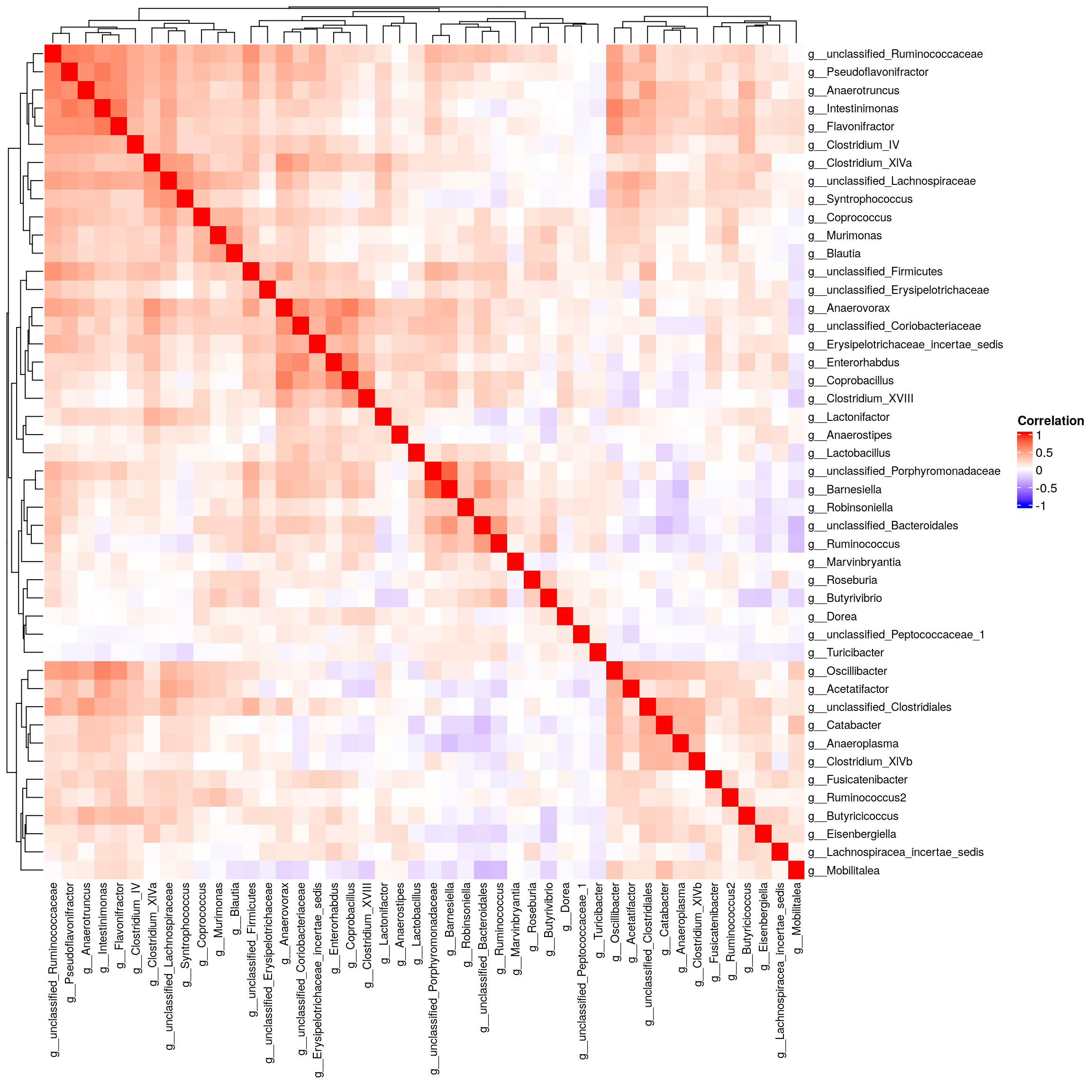
# Define a threshold for small standard deviation
sd_threshold <- 2
mat_microbe = read.csv("data/Data_repository_Bubier/microbes/cecum_sq_genus_level_counts.csv", header = TRUE) %>%
  remove_rownames %>%
  column_to_rownames(var="X") %>%
  dplyr::select(where(~ sd(.) > sd_threshold)) %>%
  dplyr::mutate(across(everything(), norm_rank_transform)) %>%
  as.matrix()

# Correlation matrix
cor.mat_microbe <- cor(mat_microbe, use = "pairwise.complete.obs")
cor.p.mat_microbe <- rcorr(mat_microbe)
cor.p.mat_microbe <- flattenCorrMatrix(cor.p.mat_microbe$r, cor.p.mat_microbe$P)
# Create the heatmap
Heatmap(
  cor.mat_microbe,
  name = "Correlation",              # Title of the legend
  col = colorRamp2(c(-1, 0, 1), c("blue", "white", "red")), # Color scale
  show_row_names = TRUE,             # Display row names
  show_column_names = TRUE,           # Display column names
  row_names_gp = gpar(fontsize = 9),
  column_names_gp = gpar(fontsize = 9)
)
| Version | Author | Date |
|---|---|---|
| 3577bf9 | xhyuo | 2025-01-08 |
#display Correlation
DT::datatable(cor.p.mat_microbe,
              filter = list(position = 'top', clear = FALSE),
              extensions = 'Buttons',
              options = list(dom = 'Blfrtip',
                             buttons = c('csv', 'excel'),
                             lengthMenu = list(c(10,25,50,-1),
                                               c(10,25,50,"All")),
                             pageLength = 40,
                             scrollY = "300px",
                             scrollX = "40px"),
              caption = htmltools::tags$caption(style = 'caption-side: top; text-align: left; color:black; font-size:200% ; Correlation of microbe abundance'))
03 Cecum co-expression module vectors (data object: mat_DO_cecum_ME) and meQTL (module eigengenes) mapping
load("data/Data_repository_Bubier/cecum_expression/qtlviewer_DO_Cecum_416_06302020.RData")

if(FALSE){
expr = dataset.DO_Cecum_416$data
DO_wgcna_gsg = goodSamplesGenes(expr)
ifelse(DO_wgcna_gsg$allOK,
       "All genes are good and all samples are good.",
       "There are bad samples or genes.")
#Finding soft threshold
powers = c(c(1:10), seq(from = 12, to=20, by=2))
DO_wgcna_sft = pickSoftThreshold(expr,
                                 powerVector = powers,
                                 networkType="signed",
                                 corFnc = bicor)
#Plotting scale-free topology fit
plot(x = DO_wgcna_sft$fitIndices$Power,
     DO_wgcna_sft$fitIndices$SFT.R.sq,
     xlab = "Soft Threshold (power)",
     ylab = "R-Squared", type ="l",
     col = "dark gray", main = "Scale Independence (all)")
text(DO_wgcna_sft$fitIndices$Power,
     DO_wgcna_sft$fitIndices$SFT.R.sq,
     labels = powers, col ="#3399CC")
abline(h = 0.9, col = "#FF3333")
#Plotting median connectivity
plot(x = DO_wgcna_sft$fitIndices$Power,
     y = DO_wgcna_sft$fitIndices$median.k,
     xlab = "Soft Threshold (powers)",
     ylab = "Median Connectivity",
     main = "Median Connectivity (all)",
     col = "dark gray", type = "l")
text(DO_wgcna_sft$fitIndices$Power, DO_wgcna_sft$fitIndices$median.k., labels = powers, col = "#3399CC")
#module
DO_modules = blockwiseModules(expr, power = 9,
                              networkType = "signed",
                              minModuleSize = 30,
                              corType= "bicor",
                              maxBlockSize = 30000,
                              numericLabels = TRUE,
                              saveTOMs = FALSE,
                              verbose = 3)
DO_colors = labels2colors(DO_modules$colors)
mat_DO_cecum_ME = DO_modules$MEs %>%
  dplyr::select(-ME0) %>%
  t() %>%
  as.matrix()
saveRDS(mat_DO_cecum_ME, file = "data/Data_repository_Bubier/cecum_expression/mat_DO_cecum_ME.RDS")

mat_DO_cecum_MM = data.frame(ID = colnames(expr),
                                module = DO_modules$colors,
                                color = DO_colors)
#annotate module membership
# Connect to the Ensembl database
ensembl <- useMart("ensembl", dataset = "mmusculus_gene_ensembl")
# list of Ensembl IDs
ensembl_ids <- mat_DO_cecum_MM$ID
# Convert Ensembl IDs to gene symbols
gene_symbols <- getBM(
  attributes = c("ensembl_gene_id", "mgi_symbol"), # Fields to retrieve
  filters = "ensembl_gene_id",                    # Type of ID to filter by
  values = ensembl_ids,                           # List of Ensembl IDs
  mart = ensembl                                   # Ensembl connection
)
# View the result
mat_DO_cecum_MM = left_join(mat_DO_cecum_MM, gene_symbols, by = c("ID" = "ensembl_gene_id"))
saveRDS(mat_DO_cecum_MM, file = "data/Data_repository_Bubier/cecum_expression/mat_DO_cecum_MM.RDS")
}

#meQTL (module eigengenes) mapping was done by cecum_meQTL.sh using cecum_meQTL.R
load("data/Data_repository_Bubier/cecum_expression/meQTL.RData")
#peaks
cecum_meQTL_peaks <- tibble(module_name = names(qtl.peaks),
                            peaks0      = qtl.peaks) %>%
  dplyr::mutate(peaks = map2(module_name, peaks0, function(x, y){
    y <- y %>%
      dplyr::mutate(lodcolumn = x) %>%
      dplyr::mutate(p.value = map_dbl(lod, function(x){mean(qtl.operm[[1]][,1] >= x)}), .after = "lod") %>%
      dplyr::mutate(marker = map2_chr(chr, pos, function(a, b){
        find_marker(map, a, b)
        }), .after = pos)
  }))
cecum_meQTL_peaks_df <- bind_rows(cecum_meQTL_peaks$peaks) %>%
  dplyr::mutate(lodcolumn = paste0("cecum_", lodcolumn))

#display cecum_meQTL_peaks_df
DT::datatable(cecum_meQTL_peaks_df[,-1],
              filter = list(position = 'top', clear = FALSE),
              extensions = 'Buttons',
              options = list(dom = 'Blfrtip',
                             buttons = c('csv', 'excel'),
                             lengthMenu = list(c(10,25,50,-1),
                                               c(10,25,50,"All")),
                             pageLength = 40,
                             scrollY = "300px",
                             scrollX = "40px"),
              caption = htmltools::tags$caption(style = 'caption-side: top; text-align: left; color:black; font-size:200% ; Table of LOD (> 6), p value, peak marker, confidence interval of cecum meQTL mapping'))
04 Striatum co-expression module vectors (data object: mat_DO_striatum_ME) and and meQTL (module eigengenes) mapping
load("data/Data_repository_Bubier/striatum_expression/core.CSNA_DO_Striatum.v3.RData")

if(FALSE){
expr = striatum$data
DO_wgcna_gsg = goodSamplesGenes(expr)
ifelse(DO_wgcna_gsg$allOK,
       "All genes are good and all samples are good.",
       "There are bad samples or genes.")
#Finding soft threshold
powers = c(c(1:10), seq(from = 12, to=20, by=2))
DO_wgcna_sft = pickSoftThreshold(expr,
                                 powerVector = powers,
                                 networkType="signed",
                                 corFnc = bicor)
#Plotting scale-free topology fit
plot(x = DO_wgcna_sft$fitIndices$Power,
     DO_wgcna_sft$fitIndices$SFT.R.sq,
     xlab = "Soft Threshold (power)",
     ylab = "R-Squared", type ="l",
     col = "dark gray", main = "Scale Independence (all)")
text(DO_wgcna_sft$fitIndices$Power,
     DO_wgcna_sft$fitIndices$SFT.R.sq,
     labels = powers, col ="#3399CC")
abline(h = 0.9, col = "#FF3333")
#Plotting median connectivity
plot(x = DO_wgcna_sft$fitIndices$Power,
     y = DO_wgcna_sft$fitIndices$median.k,
     xlab = "Soft Threshold (powers)",
     ylab = "Median Connectivity",
     main = "Median Connectivity (all)",
     col = "dark gray", type = "l")
text(DO_wgcna_sft$fitIndices$Power, DO_wgcna_sft$fitIndices$median.k., labels = powers, col = "#3399CC")
#module
DO_modules = blockwiseModules(expr, power = 3,
                              networkType = "signed",
                              minModuleSize = 30,
                              corType= "bicor",
                              maxBlockSize = 30000,
                              numericLabels = TRUE,
                              saveTOMs = FALSE,
                              verbose = 3)
DO_colors = labels2colors(DO_modules$colors)
mat_DO_striatum_ME = DO_modules$MEs %>%
  dplyr::select(-ME0) %>%
  t() %>%
  as.matrix()
saveRDS(mat_DO_striatum_ME, file = "data/Data_repository_Bubier/striatum_expression/mat_DO_striatum_ME.RDS")

mat_DO_striatum_MM = data.frame(ID = colnames(expr),
                                module = DO_modules$colors,
                                color = DO_colors)
#annotate module membership
# Connect to the Ensembl database
ensembl <- useMart("ensembl", dataset = "mmusculus_gene_ensembl")
# list of Ensembl IDs
ensembl_ids <- mat_DO_striatum_MM$ID
# Convert Ensembl IDs to gene symbols
gene_symbols <- getBM(
  attributes = c("ensembl_gene_id", "mgi_symbol"), # Fields to retrieve
  filters = "ensembl_gene_id",                    # Type of ID to filter by
  values = ensembl_ids,                           # List of Ensembl IDs
  mart = ensembl                                   # Ensembl connection
)
# View the result
mat_DO_striatum_MM = left_join(mat_DO_striatum_MM, gene_symbols, by = c("ID" = "ensembl_gene_id"))
saveRDS(mat_DO_striatum_MM, file = "data/Data_repository_Bubier/striatum_expression/mat_DO_striatum_MM.RDS")
}

#meQTL (module eigengenes) mapping was done by striatum_meQTL.sh using striatum_meQTL.R
load("data/Data_repository_Bubier/striatum_expression/meQTL.RData")
#peaks
striatum_meQTL_peaks <- tibble(module_name = names(qtl.peaks),
                            peaks0      = qtl.peaks) %>%
  dplyr::mutate(peaks = map2(module_name, peaks0, function(x, y){
    y <- y %>%
      dplyr::mutate(lodcolumn = x) %>%
      dplyr::mutate(p.value = map_dbl(lod, function(x){mean(qtl.operm[[1]][,1] >= x)}), .after = "lod") %>%
      dplyr::mutate(marker = map2_chr(chr, pos, function(a, b){
        find_marker(map, a, b)
        }), .after = pos)
  }))
striatum_meQTL_peaks_df <- bind_rows(striatum_meQTL_peaks$peaks) %>%
  dplyr::mutate(lodcolumn = paste0("striatum_", lodcolumn))

#display striatum_meQTL_peaks_df
DT::datatable(striatum_meQTL_peaks_df[,-1],
              filter = list(position = 'top', clear = FALSE),
              extensions = 'Buttons',
              options = list(dom = 'Blfrtip',
                             buttons = c('csv', 'excel'),
                             lengthMenu = list(c(10,25,50,-1),
                                               c(10,25,50,"All")),
                             pageLength = 40,
                             scrollY = "300px",
                             scrollX = "40px"),
              caption = htmltools::tags$caption(style = 'caption-side: top; text-align: left; color:black; font-size:200% ; Table of LOD (> 6), p value, peak marker, confidence interval of striatum meQTL mapping'))
1. PMCA(X, Y): X = predisposing behaviors (subset1), Y = microbe abundance
#The "X" matrix is all other traits (referred to as Predisposing Traits) except the IVSA traits (referred to as Cocaine-Seeking Traits)
num = "num1" #name of output
output_dir = paste0("output/PMCA/", num)
  if (!dir.exists(output_dir))
  {dir.create(output_dir)}

#X = predisposing behaviors (subset1)
load("data/Data_repository_Bubier/mat_predisposing_behaviors.RData")

#Y = microbe abundance
overlap.id = intersect(rownames(mat_microbe), mat_predisposing_behaviors$Mouse.ID)
y = mat_microbe[overlap.id,]

#subset mat_predisposing_behaviors
x = mat_predisposing_behaviors %>%
  dplyr::filter(Mouse.ID %in% overlap.id) %>%
  remove_rownames %>%
  column_to_rownames(var="Mouse.ID") %>%
  dplyr::select(where(~ !all(is.na(.)))) %>%
  dplyr::mutate(across(everything(), norm_rank_transform)) %>%
  dplyr::mutate(across(everything(), ~ replace(., is.na(.), 0))) %>%#replace NA with 0
  as.matrix()

# Correlation matrix
cor.x <- cor(x, use = "pairwise.complete.obs")
cor.p.x <- rcorr(x)
cor.p.x <- flattenCorrMatrix(cor.p.x$r, cor.p.x$P)
# Create the heatmap
ComplexHeatmap::Heatmap(
  cor.x,
  name = "Correlation",              # Title of the legend
  col = colorRamp2(c(-1, 0, 1), c("blue", "white", "red")), # Color scale
  show_row_names = TRUE,             # Display row names
  show_column_names = TRUE,           # Display column names
  row_names_gp = gpar(fontsize = 9),
  column_names_gp = gpar(fontsize = 9),
  row_names_side = "left",
  row_dend_side = c("right")
)-1.png)
#display Correlation
DT::datatable(cor.p.x,
              filter = list(position = 'top', clear = FALSE),
              extensions = 'Buttons',
              options = list(dom = 'Blfrtip',
                             buttons = c('csv', 'excel'),
                             lengthMenu = list(c(10,25,50,-1),
                                               c(10,25,50,"All")),
                             pageLength = 40,
                             scrollY = "300px",
                             scrollX = "40px"),
caption = htmltools::tags$caption(style = 'caption-side: top; text-align: left; color:black; font-size:200% ; Correlation of predisposing behaviors'))-3.png)
# Positive and negative associated scores
scores.real <- get.scores(mca.real$Zx,mca.real$Zy) # for associated lists
scores.neg  <- get.scores(-mca.real$Zx,mca.real$Zy) # for anti-associated lists

# for reproducibility
set.seed(B)
scores.rand <- permutation.proc(x,y,method=method,B=B) # get scores for all B permutations

# iterative step
w <- apply(mca.real$Zx,2,sd) # get starting window vector
it.result <- iterative.proc(scores.rand,alpha=alpha,w=w,method=method,by=by,rowterms=rownames(y),plot=plot,tau=0.1)-4.png)
# Print tau and the estimated FPR at each component and row of pipeline
#   NOTE: tau should NOT be the tau value you put in above. It should auto adjust to reflect your data
it.result$tau
# [1] 0.6
head(round(it.result$FPR, 3))
#       [,1]  [,2]  [,3]  [,4]  [,5]  [,6]  [,7]  [,8]  [,9] [,10] [,11] [,12]
# [1,] 0.857 0.515 0.265 0.206 0.165 0.106 0.062 0.024 0.011 0.006 0.003 0.002
# [2,] 0.665 0.364 0.187 0.150 0.126 0.094 0.075 0.054 0.038 0.023 0.013 0.009
# [3,] 0.777 0.438 0.200 0.140 0.101 0.063 0.045 0.033 0.027 0.021 0.014 0.011
# [4,] 0.758 0.427 0.202 0.147 0.108 0.066 0.047 0.033 0.028 0.022 0.014 0.011
# [5,] 0.936 0.497 0.207 0.132 0.092 0.054 0.038 0.028 0.023 0.018 0.012 0.009
# [6,] 0.956 0.507 0.211 0.135 0.093 0.054 0.037 0.027 0.022 0.017 0.011 0.008
#      [,13] [,14] [,15] [,16] [,17] [,18] [,19]
# [1,] 0.002 0.001 0.001 0.000 0.000 0.000 0.000
# [2,] 0.007 0.007 0.004 0.002 0.002 0.002 0.001
# [3,] 0.009 0.009 0.006 0.003 0.003 0.002 0.002
# [4,] 0.009 0.009 0.006 0.003 0.003 0.003 0.002
# [5,] 0.007 0.007 0.004 0.002 0.002 0.002 0.001
# [6,] 0.006 0.006 0.004 0.002 0.002 0.002 0.001

# g = list of rownames(Y) that match patterns of rownames(X)
# g[[i]][[j]]: is all the rownames(Y) that match the pattern of rownames(X)[i] when the component = j
# example: If you want to know what genes map to "LP_Dip" (row 6)
# when you use 4 components, g[[6]][[4]]
g <- match.patterns(scores.real,w=it.result$wopt, rowterms=rownames(y))

# same thing for h but h is the anti-associated rowterms(Y)
h <- match.patterns(scores.neg,w=it.result$wopt, rowterms=rownames(y))

# get int with compoent 8
#   NOTE: you may need to change this based on what you see in the "head(round(it.result$FPR, 3))"
# int_g <- get.inter(g,7)
# rownames(int_g) <- colnames(int_g) <- rownames(x)
#
# int_h <- get.inter(h,7)
# rownames(int_h) <- colnames(int_h) <- rownames(x)

# FPR for all components
fpr <- it.result$FPR
if(!is.null(dim(fpr))){
  rownames(fpr) <- rownames(x)
  colnames(fpr) <- paste0("component=", 1:ncol(fpr))
} else{
  names(fpr) <- paste0("component=", 1:length(fpr))
}

names(it.result$wopt) <- c(paste0("component=",1:length(it.result$wopt)))

result <- list(mapped = g, antimapped = h, FPR = fpr, wopt = it.result$wopt, tau = it.result$tau)

# Get associated and anti-associated matrices
associated_A <- get_adj(g)
anti_A <- get_adj(h)

# save
saveRDS(list(associated=associated_A, anti=anti_A),
        file = paste0("output/PMCA/", num, "/", "adjacency_matrices.RDS"))

# create and save edgelist and edgelist components
outdir <- paste0("output/PMCA/", num, "/", "edgelists/")
# create the outdir
if (!dir.exists(outdir))
{dir.create(outdir)}
direction <- TRUE
alpha <- 0.05
savename <- paste0("PMCA-", num)
edgelist1 <- extract_edgelist_from_adjacency_matrices(associated = associated_A,
                                                      antiassociated = anti_A,
                                                      alpha = alpha,
                                                      outdir=outdir,
                                                      direction = TRUE,
                                                      savename = savename)
# [1] "Processing entries_total_HB_do..."
# [1] "Processing light_dark_transitions_LD_do..."
# [1] "Processing pct_dist_light_LD_do..."
# [1] "Processing pct_time_light_LD_do..."
# [1] "Processing time_w_gray_do..."
# [1] "Processing time_wo_gray_do..."
# [1] "Processing amb_dist_OFT_do_bin1..."
# [1] "Processing ambulatory_distance_center_first_20_mins_do..."
# [1] "Processing ambulatory_distance_center_first_20_mins_slope_do..."
# [1] "Processing ambulatory_distance_total_first_20_mins_slope_do..."
# [1] "Processing ambulatory_time_center_first_20_mins_do..."
# [1] "Processing pct_time_center_OFT_do_bin1..."
# [1] "Processing rest_time_corner_slope_do..."
# [1] "Processing total_rest_time_corner_do..."
# [1] "Processing total_time_center_first_20_mins_do..."
# [1] "Processing entries_total_HB_do..."
# [1] "Processing light_dark_transitions_LD_do..."
# [1] "Processing pct_ambulatory_distance_light_LD_slope..."
# [1] "Processing pct_time_light_LD_slope_do..."
# [1] "Processing time_w_gray_do..."
# [1] "Processing time_wo_gray_do..."
# [1] "Processing amb_dist_OFT_do_bin1..."
# [1] "Processing ambulatory_distance_center_first_20_mins_do..."
# [1] "Processing ambulatory_distance_total_first_20_mins_do..."
# [1] "Processing ambulatory_distance_total_first_20_mins_slope_do..."
# [1] "Processing ambulatory_time_center_first_20_mins_do..."
# [1] "Processing ambulatory_time_center_first_20_mins_slope_do..."
# [1] "Processing pct_time_center_OFT_do_bin1..."
# [1] "Processing rest_time_corner_slope_do..."
# [1] "Processing total_rest_time_corner_do..."
# [1] "Processing total_time_center_first_20_mins_do..."
write.csv(edgelist1, paste0("output/PMCA/", num, "/", "edgelist_traits_acquired.csv"), row.names = F, quote = F)

# Heat maps
# set up palette
aa1 <- anti_A
aa1[which(is.na(aa1))] <- 0
gp.aa <- get.palette(aa1,center=0.25)
palette.aa <- gp.aa$pal2
pal.breaks.aa <- gp.aa$breaks
# anti-associated matrix set up for heat map
aa <- anti_A
aa[which(is.na(aa))] <- 1
# heat map
heatmap.2(t(aa),
          cexRow = 1.0, # text size
          cexCol = 1.0,
          margins=c(16,16), # figure margins
          col = palette.aa, # colors
          scale = "none", # because we already normalize
          trace = "none", # puts weird lines everywhere
          symkey=FALSE, # makes the color key show values that reflect the data
          density.info="none",
          srtCol = 45, # angle col names
main = "Anti-Associated All Traits \n")-5.png)
# Save anti heat map
jpeg(paste0("output/PMCA/", num, "/", "antiassociated_alltraits_heatmap.jpeg"), width = 1024, height = 800)
heatmap.2(t(aa),
          cexRow = 1.0, # text size
          cexCol = 1.0,
          margins=c(16,16), # figure margins
          col = palette.aa, # colors
          scale = "none", # because we already normalize
          trace = "none", # puts weird lines everywhere
          symkey=FALSE, # makes the color key show values that reflect the data
          density.info="none",
          srtCol = 45, # angle col names
          main = "Anti-Associated All Traits \n")
dev.off()
# png
#   2

# set up palette
a1 <- associated_A
a1[which(is.na(a1))] <- 0
gp.a <- get.palette(a1,center=0.25)
palette.a <- gp.a$pal2
pal.breaks.a <- gp.a$breaks
# anti-associated matrix set up for heat map
a <- associated_A
a[which(is.na(a))] <- 1

heatmap.2(t(a),
          cexRow = 1.0, # text size
          cexCol = 1.0,
          margins=c(16,16), # figure margins
          col = palette.a, # colors
          scale = "none", # because we already normalize
          trace = "none", # puts weird lines everywhere
          symkey=FALSE, # makes the color key show values that reflect the data
          density.info="none",
          srtCol = 45, # angle col names
main = "Associated All Traits \n")-6.png)
# Save assoc heat map
jpeg(paste0("output/PMCA/", num, "/", "associated_alltraits_heatmap.jpeg"), width = 1024, height = 800)
heatmap.2(t(a),
          cexRow = 1.0, # text size
          cexCol = 1.0,
          margins=c(16,16), # figure margins
          col = palette.a, # colors
          scale = "none", # because we already normalize
          trace = "none", # puts weird lines everywhere
          symkey=FALSE, # makes the color key show values that reflect the data
          density.info="none",
          srtCol = 45, # angle col names
          main = "Associated All Traits \n")
dev.off()
# png
#   2

#turn edgelist into heatmap
edgelist1_mat <- edgelist1 %>%
  dplyr::mutate(fpr = ifelse(direction == "negative", -fpr, fpr)) %>%
  dplyr::mutate(fpr = ifelse(direction == "negative" & fpr == 0, -0.0001, fpr)) %>%
  dplyr::mutate(fpr = ifelse(direction == "positive" & fpr == 0, 0.0001, fpr)) %>%
  dplyr::select(-direction) %>%
  pivot_wider(
    data = .,
    names_from = yname, # Column to create new column names
    values_from = fpr    # Column to populate the values
  ) %>%
  column_to_rownames("xname") %>%
  as.matrix()
ComplexHeatmap::Heatmap(edgelist1_mat,
                        na_col = "white",
                        name = "FPR",
                        column_title = paste0(num, " PMCA heatmap of positive/negative edge"),
                        col = colorRamp2(c(-0.05, -0.0001, 0, 0.0001, 0.05), c("white", "blue", "black", "red", "white")), # Color scale
                        row_names_side = "left",
#                        row_names_max_width = unit(8, "cm"),
                        row_names_gp = gpar(fontsize = 10),
                        column_names_gp = gpar(fontsize = 10),
                        cluster_rows = F,
                        cluster_columns = F
)-7.png)
| Version | Author | Date |
|---|---|---|
| f7325c7 | xhyuo | 2025-01-15 |
# display edgelist
DT::datatable(edgelist1,
              filter = list(position = 'top', clear = FALSE),
              extensions = 'Buttons',
              options = list(dom = 'Blfrtip',
                             buttons = c('csv', 'excel'),
                             lengthMenu = list(c(10,25,50,-1),
                                               c(10,25,50,"All")),
                             pageLength = 40,
                             scrollY = "300px",
                             scrollX = "40px"),
              caption = htmltools::tags$caption(style = 'caption-side: top; text-align: left; color:black; font-size:200% ;', paste0(num, " PMCA edgelist")))
2. PMCA(X, Y): X = microbe abundance (subset1), Y = striatum co-expression module vectors
num = "num2" #name of output
output_dir = paste0("output/PMCA/", num)
if (!dir.exists(output_dir))
  {dir.create(output_dir)}

mat_DO_striatum_ME <- readRDS("data/Data_repository_Bubier/striatum_expression/mat_DO_striatum_ME.RDS")
rownames(mat_DO_striatum_ME) <- paste0("striatum_", rownames(mat_DO_striatum_ME))

overlap.id = intersect(rownames(mat_microbe), colnames(mat_DO_striatum_ME))
x = mat_microbe[overlap.id,] %>%
  t() %>%
  as.matrix()
y = mat_DO_striatum_ME[, overlap.id]
all.equal(colnames(x), colnames(y))
# [1] TRUE

# Calculate Z_x, Z_y, and sigma for matrices pipeline and novelty
mca.real <- get.mca(x,y)
#plot(mca.real$sigma)

#find best by
find_best_by(sigma_data = mca.real$sigma)
# [1] 9
#find_best_by()

# ‘by’ should be this ‘find_by_by’ value
# Calculate the FPR for each rowterm of pipeline
by<- find_best_by(); method <- "each"; B <- 1000; alpha <- 0.05; plot <- TRUE-1.png)
# Positive and negative associated scores
scores.real <- get.scores(mca.real$Zx,mca.real$Zy) # for associated lists
scores.neg  <- get.scores(-mca.real$Zx,mca.real$Zy) # for anti-associated lists

# for reproducibility
set.seed(B)
scores.rand <- permutation.proc(x,y,method=method,B=B) # get scores for all B permutations

# iterative step
w <- apply(mca.real$Zx,2,sd) # get starting window vector
it.result <- iterative.proc(scores.rand,alpha=alpha,w=w,method=method,by=by,rowterms=rownames(y),plot=plot,tau=0.1)-2.png)
# Print tau and the estimated FPR at each component and row of pipeline
#   NOTE: tau should NOT be the tau value you put in above. It should auto adjust to reflect your data
it.result$tau
# [1] 0.5
head(round(it.result$FPR, 3))
#       [,1]  [,2]  [,3]  [,4]  [,5]  [,6]  [,7]  [,8]  [,9] [,10] [,11] [,12]
# [1,] 0.450 0.322 0.220 0.104 0.062 0.043 0.027 0.022 0.016 0.015 0.014 0.012
# [2,] 0.557 0.311 0.185 0.083 0.048 0.034 0.020 0.016 0.012 0.011 0.010 0.009
# [3,] 0.735 0.489 0.309 0.139 0.077 0.050 0.025 0.019 0.011 0.010 0.008 0.006
# [4,] 0.443 0.297 0.198 0.095 0.056 0.041 0.025 0.020 0.016 0.015 0.014 0.011
# [5,] 0.600 0.469 0.298 0.122 0.061 0.040 0.022 0.016 0.010 0.009 0.008 0.005
# [6,] 0.486 0.369 0.249 0.114 0.065 0.044 0.025 0.020 0.014 0.013 0.012 0.010
#      [,13] [,14] [,15] [,16] [,17] [,18] [,19] [,20] [,21] [,22]
# [1,] 0.011 0.008 0.007 0.006 0.005 0.004 0.004 0.003 0.003 0.003
# [2,] 0.008 0.006 0.006 0.005 0.004 0.004 0.003 0.003 0.003 0.003
# [3,] 0.004 0.003 0.002 0.001 0.001 0.000 0.000 0.000 0.000 0.000
# [4,] 0.010 0.008 0.007 0.006 0.006 0.005 0.004 0.004 0.004 0.004
# [5,] 0.004 0.002 0.002 0.002 0.001 0.001 0.000 0.000 0.000 0.000
# [6,] 0.008 0.006 0.006 0.004 0.004 0.003 0.003 0.002 0.002 0.002

# g = list of rownames(Y) that match patterns of rownames(X)
# g[[i]][[j]]: is all the rownames(Y) that match the pattern of rownames(X)[i] when the component = j
# example: If you want to know what genes map to "LP_Dip" (row 6)
# when you use 4 components, g[[6]][[4]]
g <- match.patterns(scores.real,w=it.result$wopt, rowterms=rownames(y))

# same thing for h but h is the anti-associated rowterms(Y)
h <- match.patterns(scores.neg,w=it.result$wopt, rowterms=rownames(y))

# get int with compoent 8
#   NOTE: you may need to change this based on what you see in the "head(round(it.result$FPR, 3))"
# int_g <- get.inter(g,7)
# rownames(int_g) <- colnames(int_g) <- rownames(x)
#
# int_h <- get.inter(h,7)
# rownames(int_h) <- colnames(int_h) <- rownames(x)

# FPR for all components
fpr <- it.result$FPR
if(!is.null(dim(fpr))){
  rownames(fpr) <- rownames(x)
  colnames(fpr) <- paste0("component=", 1:ncol(fpr))
} else{
  names(fpr) <- paste0("component=", 1:length(fpr))
}

names(it.result$wopt) <- c(paste0("component=",1:length(it.result$wopt)))

result <- list(mapped = g, antimapped = h, FPR = fpr, wopt = it.result$wopt, tau = it.result$tau)

# Get associated and anti-associated matrices
associated_A <- get_adj(g)
anti_A <- get_adj(h)

# save
saveRDS(list(associated=associated_A, anti=anti_A),
        file = paste0("output/PMCA/", num, "/", "adjacency_matrices.RDS"))

# create and save edgelist and edgelist components
outdir <- paste0("output/PMCA/", num, "/", "edgelists/")
# create the outdir
if (!dir.exists(outdir))
{dir.create(outdir)}
direction <- TRUE
alpha <- 0.05
savename <- paste0("PMCA-", num)
edgelist2 <- extract_edgelist_from_adjacency_matrices(associated = associated_A,
                                                      antiassociated = anti_A,
                                                      alpha = alpha,
                                                      outdir=outdir,
                                                      direction = TRUE,
                                                      savename = savename)
# [1] "Processing g__Syntrophococcus..."
# [1] "Processing g__unclassified_Bacteroidales..."
# [1] "Processing g__Turicibacter..."
# [1] "Processing g__Fusicatenibacter..."
# [1] "Processing g__Clostridium_IV..."
# [1] "Processing g__Clostridium_XlVa..."
# [1] "Processing g__Anaerovorax..."
# [1] "Processing g__Oscillibacter..."
# [1] "Processing g__Flavonifractor..."
# [1] "Processing g__Blautia..."
# [1] "Processing g__Eisenbergiella..."
# [1] "Processing g__unclassified_Firmicutes..."
# [1] "Processing g__Mobilitalea..."
# [1] "Processing g__Butyrivibrio..."
# [1] "Processing g__Pseudoflavonifractor..."
# [1] "Processing g__unclassified_Clostridiales..."
# [1] "Processing g__unclassified_Coriobacteriaceae..."
# [1] "Processing g__Coprococcus..."
# [1] "Processing g__Intestinimonas..."
# [1] "Processing g__Lactobacillus..."
# [1] "Processing g__Anaerotruncus..."
# [1] "Processing g__unclassified_Lachnospiraceae..."
# [1] "Processing g__Clostridium_XVIII..."
# [1] "Processing g__Enterorhabdus..."
# [1] "Processing g__Lachnospiracea_incertae_sedis..."
# [1] "Processing g__Catabacter..."
# [1] "Processing g__Coprobacillus..."
# [1] "Processing g__Murimonas..."
# [1] "Processing g__Lactonifactor..."
# [1] "Processing g__Marvinbryantia..."
# [1] "Processing g__Ruminococcus2..."
# [1] "Processing g__Anaeroplasma..."
# [1] "Processing g__Anaerostipes..."
# [1] "Processing g__Robinsoniella..."
# [1] "Processing g__Erysipelotrichaceae_incertae_sedis..."
# [1] "Processing g__unclassified_Ruminococcaceae..."
# [1] "Processing g__Dorea..."
# [1] "Processing g__unclassified_Peptococcaceae_1..."
# [1] "Processing g__Syntrophococcus..."
# [1] "Processing g__unclassified_Bacteroidales..."
# [1] "Processing g__Fusicatenibacter..."
# [1] "Processing g__Acetatifactor..."
# [1] "Processing g__Clostridium_IV..."
# [1] "Processing g__Oscillibacter..."
# [1] "Processing g__Flavonifractor..."
# [1] "Processing g__Butyricicoccus..."
# [1] "Processing g__Blautia..."
# [1] "Processing g__Eisenbergiella..."
# [1] "Processing g__Mobilitalea..."
# [1] "Processing g__Butyrivibrio..."
# [1] "Processing g__Ruminococcus..."
# [1] "Processing g__Pseudoflavonifractor..."
# [1] "Processing g__unclassified_Clostridiales..."
# [1] "Processing g__unclassified_Coriobacteriaceae..."
# [1] "Processing g__Coprococcus..."
# [1] "Processing g__Intestinimonas..."
# [1] "Processing g__Lactobacillus..."
# [1] "Processing g__Anaerotruncus..."
# [1] "Processing g__unclassified_Lachnospiraceae..."
# [1] "Processing g__Clostridium_XVIII..."
# [1] "Processing g__Enterorhabdus..."
# [1] "Processing g__Lachnospiracea_incertae_sedis..."
# [1] "Processing g__Catabacter..."
# [1] "Processing g__unclassified_Erysipelotrichaceae..."
# [1] "Processing g__Coprobacillus..."
# [1] "Processing g__Anaeroplasma..."
# [1] "Processing g__Anaerostipes..."
# [1] "Processing g__Robinsoniella..."
# [1] "Processing g__Erysipelotrichaceae_incertae_sedis..."
# [1] "Processing g__unclassified_Ruminococcaceae..."
# [1] "Processing g__Dorea..."
# [1] "Processing g__unclassified_Peptococcaceae_1..."
write.csv(edgelist2, paste0("output/PMCA/", num, "/", "edgelist_traits_acquired.csv"), row.names = F, quote = F)

# Heat maps
# set up palette
aa1 <- anti_A
aa1[which(is.na(aa1))] <- 0
gp.aa <- get.palette(aa1,center=0.25)
palette.aa <- gp.aa$pal2
pal.breaks.aa <- gp.aa$breaks
# anti-associated matrix set up for heat map
aa <- anti_A
aa[which(is.na(aa))] <- 1
# heat map
heatmap.2(t(aa),
          cexRow = 1.0, # text size
          cexCol = 1.0,
          margins=c(16,16), # figure margins
          col = palette.aa, # colors
          scale = "none", # because we already normalize
          trace = "none", # puts weird lines everywhere
          symkey=FALSE, # makes the color key show values that reflect the data
          density.info="none",
          srtCol = 45, # angle col names
main = "Anti-Associated All Traits \n")-3.png)
# Save anti heat map
jpeg(paste0("output/PMCA/", num, "/", "antiassociated_alltraits_heatmap.jpeg"), width = 1024, height = 800)
heatmap.2(t(aa),
          cexRow = 1.0, # text size
          cexCol = 1.0,
          margins=c(16,16), # figure margins
          col = palette.aa, # colors
          scale = "none", # because we already normalize
          trace = "none", # puts weird lines everywhere
          symkey=FALSE, # makes the color key show values that reflect the data
          density.info="none",
          srtCol = 45, # angle col names
          main = "Anti-Associated All Traits \n")
dev.off()
# png
#   2

# set up palette
a1 <- associated_A
a1[which(is.na(a1))] <- 0
gp.a <- get.palette(a1,center=0.25)
palette.a <- gp.a$pal2
pal.breaks.a <- gp.a$breaks
# anti-associated matrix set up for heat map
a <- associated_A
a[which(is.na(a))] <- 1

heatmap.2(t(a),
          cexRow = 1.0, # text size
          cexCol = 1.0,
          margins=c(16,16), # figure margins
          col = palette.a, # colors
          scale = "none", # because we already normalize
          trace = "none", # puts weird lines everywhere
          symkey=FALSE, # makes the color key show values that reflect the data
          density.info="none",
          srtCol = 45, # angle col names
main = "Associated All Traits \n")-4.png)
# Save assoc heat map
jpeg(paste0("output/PMCA/", num, "/", "associated_alltraits_heatmap.jpeg"), width = 1024, height = 800)
heatmap.2(t(a),
          cexRow = 1.0, # text size
          cexCol = 1.0,
          margins=c(16,16), # figure margins
          col = palette.a, # colors
          scale = "none", # because we already normalize
          trace = "none", # puts weird lines everywhere
          symkey=FALSE, # makes the color key show values that reflect the data
          density.info="none",
          srtCol = 45, # angle col names
          main = "Associated All Traits \n")
dev.off()
# png
#   2

#turn edgelist into heatmap
edgelist2_mat <- edgelist2 %>%
  dplyr::mutate(fpr = ifelse(direction == "negative", -fpr, fpr)) %>%
  dplyr::mutate(fpr = ifelse(direction == "negative" & fpr == 0, -0.0001, fpr)) %>%
  dplyr::mutate(fpr = ifelse(direction == "positive" & fpr == 0, 0.0001, fpr)) %>%
  dplyr::select(-direction) %>%
  pivot_wider(
    data = .,
    names_from = yname, # Column to create new column names
    values_from = fpr    # Column to populate the values
  ) %>%
  column_to_rownames("xname") %>%
  as.matrix()
ComplexHeatmap::Heatmap(edgelist2_mat,
                        na_col = "white",
                        name = "FPR",
                        column_title = paste0(num, " PMCA heatmap of positive/negative edge"),
                        col = colorRamp2(c(-0.05, -0.0001, 0, 0.0001, 0.05), c("white", "blue", "black", "red", "white")), # Color scale
                        row_names_side = "left",
#                        row_names_max_width = unit(8, "cm"),
                        row_names_gp = gpar(fontsize = 10),
                        column_names_gp = gpar(fontsize = 10),
                        cluster_rows = F,
                        cluster_columns = F
)-5.png)
| Version | Author | Date |
|---|---|---|
| f7325c7 | xhyuo | 2025-01-15 |
# display edgelist
DT::datatable(edgelist2,
              filter = list(position = 'top', clear = FALSE),
              extensions = 'Buttons',
              options = list(dom = 'Blfrtip',
                             buttons = c('csv', 'excel'),
                             lengthMenu = list(c(10,25,50,-1),
                                               c(10,25,50,"All")),
                             pageLength = 40,
                             scrollY = "300px",
                             scrollX = "40px"),
caption = htmltools::tags$caption(style = 'caption-side: top; text-align: left; color:black; font-size:200% ;', paste0(num, " PMCA edgelist")))3. PMCA(X, Y): X = microbe abundance (subset1), Y = cecum co-expression module vectors
num = "num3" #name of output
output_dir = paste0("output/PMCA/", num)
if (!dir.exists(output_dir))
{dir.create(output_dir)}

#X = microbe abundance
#Y = cecum co-expression module vectors
#mat_DO_cecum_ME
mat_DO_cecum_ME = readRDS("data/Data_repository_Bubier/cecum_expression/mat_DO_cecum_ME.RDS")
rownames(mat_DO_cecum_ME) <- paste0("cecum_", rownames(mat_DO_cecum_ME))

#mat_DO_cecum_MM
mat_DO_cecum_MM = readRDS("data/Data_repository_Bubier/cecum_expression/mat_DO_cecum_MM.RDS")

#remove ME0 grey module and subset DO mice with intersetion with x
overlap.id = intersect(rownames(mat_microbe), colnames(mat_DO_cecum_ME)) #264 DO mice
y = mat_DO_cecum_ME %>%
  .[,overlap.id]

#subset x
x = mat_microbe[overlap.id,] %>%
  t() %>%
  as.matrix()
all.equal(colnames(x), colnames(y))
# [1] TRUE

# Calculate Z_x, Z_y, and sigma for matrices pipeline and novelty
mca.real <- get.mca(x,y)
#plot(mca.real$sigma)

#find best by
find_best_by(sigma_data = mca.real$sigma)
# [1] 11
#find_best_by()

# ‘by’ should be this ‘find_by_by’ value
# Calculate the FPR for each rowterm of pipeline
by<- find_best_by(); method <- "each"; B <- 1000; alpha <- 0.05; plot <- TRUE-1.png)
# Positive and negative associated scores
scores.real <- get.scores(mca.real$Zx,mca.real$Zy) # for associated lists
scores.neg  <- get.scores(-mca.real$Zx,mca.real$Zy) # for anti-associated lists

# for reproducibility
set.seed(B)
scores.rand <- permutation.proc(x,y,method=method,B=B) # get scores for all B permutations

# iterative step
w <- apply(mca.real$Zx,2,sd) # get starting window vector
it.result <- iterative.proc(scores.rand,alpha=alpha,w=w,method=method,by=by,rowterms=rownames(y),plot=plot,tau=0.1)-2.png)
# Print tau and the estimated FPR at each component and row of pipeline
#   NOTE: tau should NOT be the tau value you put in above. It should auto adjust to reflect your data
it.result$tau
# [1] 0.5
head(round(it.result$FPR, 3))
#       [,1]  [,2]  [,3]  [,4]  [,5]  [,6]  [,7]  [,8]  [,9] [,10] [,11] [,12]
# [1,] 0.460 0.272 0.239 0.186 0.124 0.072 0.044 0.036 0.027 0.020 0.018 0.016
# [2,] 0.576 0.258 0.211 0.160 0.102 0.058 0.036 0.030 0.021 0.014 0.012 0.011
# [3,] 0.729 0.427 0.361 0.260 0.159 0.081 0.042 0.029 0.018 0.011 0.007 0.006
# [4,] 0.458 0.254 0.222 0.174 0.116 0.067 0.041 0.034 0.026 0.018 0.015 0.014
# [5,] 0.591 0.391 0.336 0.243 0.141 0.072 0.039 0.026 0.017 0.011 0.009 0.007
# [6,] 0.493 0.319 0.280 0.208 0.131 0.069 0.040 0.031 0.022 0.016 0.013 0.011
#      [,13] [,14] [,15] [,16] [,17] [,18]
# [1,] 0.015 0.013 0.012 0.011 0.010 0.009
# [2,] 0.009 0.008 0.007 0.006 0.006 0.005
# [3,] 0.004 0.002 0.002 0.001 0.001 0.000
# [4,] 0.012 0.011 0.010 0.009 0.008 0.007
# [5,] 0.005 0.004 0.003 0.002 0.002 0.002
# [6,] 0.010 0.008 0.007 0.006 0.005 0.004

# g = list of rownames(Y) that match patterns of rownames(X)
# g[[i]][[j]]: is all the rownames(Y) that match the pattern of rownames(X)[i] when the component = j
# example: If you want to know what genes map to "LP_Dip" (row 6)
# when you use 4 components, g[[6]][[4]]
g <- match.patterns(scores.real,w=it.result$wopt, rowterms=rownames(y))

# same thing for h but h is the anti-associated rowterms(Y)
h <- match.patterns(scores.neg,w=it.result$wopt, rowterms=rownames(y))

# get int with compoent 8
#   NOTE: you may need to change this based on what you see in the "head(round(it.result$FPR, 3))"
# int_g <- get.inter(g,7)
# rownames(int_g) <- colnames(int_g) <- rownames(x)
#
# int_h <- get.inter(h,7)
# rownames(int_h) <- colnames(int_h) <- rownames(x)

# FPR for all components
fpr <- it.result$FPR
if(!is.null(dim(fpr))){
  rownames(fpr) <- rownames(x)
  colnames(fpr) <- paste0("component=", 1:ncol(fpr))
  } else{
    names(fpr) <- paste0("component=", 1:length(fpr))
    }
names(it.result$wopt) <- c(paste0("component=",1:length(it.result$wopt)))
result <- list(mapped = g, antimapped = h, FPR = fpr, wopt = it.result$wopt, tau = it.result$tau)

# Get associated and anti-associated matrices
associated_A <- get_adj(g)
anti_A <- get_adj(h)

# save
saveRDS(list(associated=associated_A, anti=anti_A),
        file = paste0("output/PMCA/", num, "/", "adjacency_matrices.RDS"))

# create and save edgelist and edgelist components
outdir <- paste0("output/PMCA/", num, "/", "edgelists/")
#create the outdir
if (!dir.exists(outdir))
  {dir.create(outdir)}
direction <- TRUE
alpha <- 0.05
savename <- paste0("PMCA-", num)
edgelist3 <- extract_edgelist_from_adjacency_matrices(associated = associated_A,
                                                                   antiassociated = anti_A,
                                                                   alpha = alpha,
                                                                   outdir=outdir,
                                                                   direction = TRUE,
                                                                   savename = savename)
# [1] "Processing g__unclassified_Bacteroidales..."
# [1] "Processing g__Clostridium_XlVa..."
# [1] "Processing g__Anaerovorax..."
# [1] "Processing g__Flavonifractor..."
# [1] "Processing g__Eisenbergiella..."
# [1] "Processing g__unclassified_Firmicutes..."
# [1] "Processing g__Mobilitalea..."
# [1] "Processing g__Butyrivibrio..."
# [1] "Processing g__Pseudoflavonifractor..."
# [1] "Processing g__unclassified_Coriobacteriaceae..."
# [1] "Processing g__Intestinimonas..."
# [1] "Processing g__Lactobacillus..."
# [1] "Processing g__Anaerotruncus..."
# [1] "Processing g__Clostridium_XVIII..."
# [1] "Processing g__Enterorhabdus..."
# [1] "Processing g__Catabacter..."
# [1] "Processing g__Marvinbryantia..."
# [1] "Processing g__Anaerostipes..."
# [1] "Processing g__Robinsoniella..."
# [1] "Processing g__Erysipelotrichaceae_incertae_sedis..."
# [1] "Processing g__unclassified_Ruminococcaceae..."
# [1] "Processing g__unclassified_Peptococcaceae_1..."
# [1] "Processing g__unclassified_Bacteroidales..."
# [1] "Processing g__Turicibacter..."
# [1] "Processing g__Fusicatenibacter..."
# [1] "Processing g__Acetatifactor..."
# [1] "Processing g__Clostridium_XlVb..."
# [1] "Processing g__Anaerovorax..."
# [1] "Processing g__Butyricicoccus..."
# [1] "Processing g__Eisenbergiella..."
# [1] "Processing g__unclassified_Firmicutes..."
# [1] "Processing g__Mobilitalea..."
# [1] "Processing g__unclassified_Coriobacteriaceae..."
# [1] "Processing g__Lactobacillus..."
# [1] "Processing g__Clostridium_XVIII..."
# [1] "Processing g__Enterorhabdus..."
# [1] "Processing g__Lachnospiracea_incertae_sedis..."
# [1] "Processing g__Catabacter..."
# [1] "Processing g__Murimonas..."
# [1] "Processing g__Marvinbryantia..."
# [1] "Processing g__Anaeroplasma..."
# [1] "Processing g__Erysipelotrichaceae_incertae_sedis..."
write.csv(edgelist3, paste0("output/PMCA/", num, "/", "edgelist_traits_acquired.csv"), row.names = F, quote = F)

#Heat maps
# set up palette
aa1 <- anti_A
aa1[which(is.na(aa1))] <- 0
gp.aa <- get.palette(aa1,center=0.25)
palette.aa <- gp.aa$pal2
pal.breaks.aa <- gp.aa$breaks
# anti-associated matrix set up for heat map
aa <- anti_A
aa[which(is.na(aa))] <- 1
# heat map
heatmap.2(t(aa),
          cexRow = 1.0, # text size
          cexCol = 1.0,
          margins=c(16,16), # figure margins
          col = palette.aa, # colors
          scale = "none", # because we already normalize
          trace = "none", # puts weird lines everywhere
          symkey=FALSE, # makes the color key show values that reflect the data
          density.info="none",
          srtCol = 45, # angle col names
main = "Anti-Associated All Traits \n")-3.png)
# Save anti heat map
jpeg(paste0("output/PMCA/", num, "/", "antiassociated_alltraits_heatmap.jpeg"), width = 1024, height = 800)
heatmap.2(t(aa),
          cexRow = 1.0, # text size
          cexCol = 1.0,
          margins=c(16,16), # figure margins
          col = palette.aa, # colors
          scale = "none", # because we already normalize
          trace = "none", # puts weird lines everywhere
          symkey=FALSE, # makes the color key show values that reflect the data
          density.info="none",
          srtCol = 45, # angle col names
          main = "Anti-Associated All Traits \n")
dev.off()
# png
#   2

# set up palette
a1 <- associated_A
a1[which(is.na(a1))] <- 0
gp.a <- get.palette(a1,center=0.25)
palette.a <- gp.a$pal2
pal.breaks.a <- gp.a$breaks
# anti-associated matrix set up for heat map
a <- associated_A
a[which(is.na(a))] <- 1

heatmap.2(t(a),
          cexRow = 1.0, # text size
          cexCol = 1.0,
          margins=c(16,16), # figure margins
          col = palette.a, # colors
          scale = "none", # because we already normalize
          trace = "none", # puts weird lines everywhere
          symkey=FALSE, # makes the color key show values that reflect the data
          density.info="none",
          srtCol = 45, # angle col names
main = "Associated All Traits \n")-4.png)
# Save assoc heat map
jpeg(paste0("output/PMCA/", num, "/", "associated_alltraits_heatmap.jpeg"), width = 1024, height = 800)
heatmap.2(t(a),
          cexRow = 1.0, # text size
          cexCol = 1.0,
          margins=c(16,16), # figure margins
          col = palette.a, # colors
          scale = "none", # because we already normalize
          trace = "none", # puts weird lines everywhere
          symkey=FALSE, # makes the color key show values that reflect the data
          density.info="none",
          srtCol = 45, # angle col names
          main = "Associated All Traits \n")
dev.off()
# png
#   2

#turn edgelist into heatmap
edgelist3_mat <- edgelist3 %>%
  dplyr::mutate(fpr = ifelse(direction == "negative", -fpr, fpr)) %>%
  dplyr::mutate(fpr = ifelse(direction == "negative" & fpr == 0, -0.0001, fpr)) %>%
  dplyr::mutate(fpr = ifelse(direction == "positive" & fpr == 0, 0.0001, fpr)) %>%
  dplyr::select(-direction) %>%
  pivot_wider(
    data = .,
    names_from = yname, # Column to create new column names
    values_from = fpr    # Column to populate the values
  ) %>%
  column_to_rownames("xname") %>%
  as.matrix()
ComplexHeatmap::Heatmap(edgelist3_mat,
                        na_col = "white",
                        name = "FPR",
                        column_title = paste0(num, " PMCA heatmap of positive/negative edge"),
                        col = colorRamp2(c(-0.05, -0.0001, 0, 0.0001, 0.05), c("white", "blue", "black", "red", "white")), # Color scale
                        row_names_side = "left",
#                        row_names_max_width = unit(8, "cm"),
                        row_names_gp = gpar(fontsize = 10),
                        column_names_gp = gpar(fontsize = 10),
                        cluster_rows = F,
                        cluster_columns = F
)-5.png)
| Version | Author | Date |
|---|---|---|
| f7325c7 | xhyuo | 2025-01-15 |
#display edgelist
DT::datatable(edgelist3,
              filter = list(position = 'top', clear = FALSE),
              extensions = 'Buttons',
              options = list(dom = 'Blfrtip',
                             buttons = c('csv', 'excel'),
                             lengthMenu = list(c(10,25,50,-1),
                                               c(10,25,50,"All")),
                             pageLength = 40,
                             scrollY = "300px",
                             scrollX = "40px"),
caption = htmltools::tags$caption(style = 'caption-side: top; text-align: left; color:black; font-size:200% ;',paste0(num, " PMCA edgelist")))4. PMCA(X, Y): X = cecum co-expression module vectors, Y = striatum co-expression module vectors
num = "num4" #name of output
output_dir = paste0("output/PMCA/", num)
if (!dir.exists(output_dir))
{dir.create(output_dir)}

#X = cecum co-expression module vectors
mat_DO_cecum_ME <- readRDS("data/Data_repository_Bubier/cecum_expression/mat_DO_cecum_ME.RDS")
rownames(mat_DO_cecum_ME) <- paste0("cecum_", rownames(mat_DO_cecum_ME))

#Y = striatum co-expression module vectors
mat_DO_striatum_ME <- readRDS("data/Data_repository_Bubier/striatum_expression/mat_DO_striatum_ME.RDS")
rownames(mat_DO_striatum_ME) <- paste0("striatum_", rownames(mat_DO_striatum_ME))

overlap.id = intersect(colnames(mat_DO_cecum_ME), colnames(mat_DO_striatum_ME))

#subset to get x and y
x = mat_DO_cecum_ME[, overlap.id]
y = mat_DO_striatum_ME[, overlap.id]
all.equal(colnames(x), colnames(y))
# [1] TRUE

# Calculate Z_x, Z_y, and sigma for matrices pipeline and novelty
mca.real <- get.mca(x,y)
#plot(mca.real$sigma)

#find best by
find_best_by(sigma_data = mca.real$sigma)
# [1] 5
#find_best_by()

# ‘by’ should be this ‘find_by_by’ value
# Calculate the FPR for each rowterm of pipeline
by<- find_best_by(); method <- "each"; B <- 1000; alpha <- 0.05; plot <- TRUE-1.png)
# Positive and negative associated scores
scores.real <- get.scores(mca.real$Zx,mca.real$Zy) # for associated lists
scores.neg  <- get.scores(-mca.real$Zx,mca.real$Zy) # for anti-associated lists

# for reproducibility
set.seed(B)
scores.rand <- permutation.proc(x,y,method=method,B=B) # get scores for all B permutations

# iterative step
w <- apply(mca.real$Zx,2,sd) # get starting window vector
it.result <- iterative.proc(scores.rand,alpha=alpha,w=w,method=method,by=by,rowterms=rownames(y),plot=plot,tau=0.1)-2.png)
# Print tau and the estimated FPR at each component and row of pipeline
#   NOTE: tau should NOT be the tau value you put in above. It should auto adjust to reflect your data
it.result$tau
# [1] 1.1
head(round(it.result$FPR, 3))
#       [,1]  [,2]  [,3]  [,4]  [,5]  [,6]  [,7]  [,8]  [,9] [,10] [,11] [,12]
# [1,] 0.262 0.161 0.093 0.067 0.036 0.013 0.007 0.004 0.002 0.001 0.001 0.001
# [2,] 0.254 0.148 0.079 0.059 0.037 0.016 0.011 0.007 0.005 0.003 0.002 0.002
# [3,] 0.234 0.133 0.077 0.061 0.039 0.017 0.012 0.009 0.007 0.004 0.004 0.004
# [4,] 0.297 0.161 0.071 0.037 0.013 0.002 0.001 0.000 0.000 0.000 0.000 0.000
# [5,] 0.295 0.146 0.062 0.038 0.018 0.006 0.003 0.002 0.001 0.000 0.000 0.000
# [6,] 0.293 0.139 0.059 0.041 0.022 0.008 0.005 0.003 0.002 0.001 0.001 0.001
#      [,13] [,14] [,15] [,16] [,17] [,18]
# [1,] 0.001 0.000 0.000 0.000 0.000 0.000
# [2,] 0.002 0.001 0.001 0.001 0.001 0.000
# [3,] 0.003 0.002 0.002 0.002 0.002 0.001
# [4,] 0.000 0.000 0.000 0.000 0.000 0.000
# [5,] 0.000 0.000 0.000 0.000 0.000 0.000
# [6,] 0.001 0.001 0.000 0.000 0.000 0.000

# g = list of rownames(Y) that match patterns of rownames(X)
# g[[i]][[j]]: is all the rownames(Y) that match the pattern of rownames(X)[i] when the component = j
# example: If you want to know what genes map to "LP_Dip" (row 6)
# when you use 4 components, g[[6]][[4]]
g <- match.patterns(scores.real,w=it.result$wopt, rowterms=rownames(y))

# same thing for h but h is the anti-associated rowterms(Y)
h <- match.patterns(scores.neg,w=it.result$wopt, rowterms=rownames(y))

# get int with compoent 8
#   NOTE: you may need to change this based on what you see in the "head(round(it.result$FPR, 3))"
# int_g <- get.inter(g,7)
# rownames(int_g) <- colnames(int_g) <- rownames(x)
#
# int_h <- get.inter(h,7)
# rownames(int_h) <- colnames(int_h) <- rownames(x)

# FPR for all components
fpr <- it.result$FPR
if(!is.null(dim(fpr))){
  rownames(fpr) <- rownames(x)
  colnames(fpr) <- paste0("component=", 1:ncol(fpr))
} else{
  names(fpr) <- paste0("component=", 1:length(fpr))
}
names(it.result$wopt) <- c(paste0("component=",1:length(it.result$wopt)))
result <- list(mapped = g, antimapped = h, FPR = fpr, wopt = it.result$wopt, tau = it.result$tau)

# Get associated and anti-associated matrices
associated_A <- get_adj(g)
anti_A <- get_adj(h)

# save
saveRDS(list(associated=associated_A, anti=anti_A),
        file = paste0("output/PMCA/", num, "/", "adjacency_matrices.RDS"))

# create and save edgelist and edgelist components
outdir <- paste0("output/PMCA/", num, "/", "edgelists/")
#create the outdir
if (!dir.exists(outdir))
{dir.create(outdir)}
direction <- TRUE
alpha <- 0.05
savename <- paste0("PMCA-", num)
edgelist4 <- extract_edgelist_from_adjacency_matrices(associated = associated_A,
                                                      antiassociated = anti_A,
                                                      alpha = alpha,
                                                      outdir=outdir,
                                                      direction = TRUE,
                                                      savename = savename)
# [1] "Processing cecum_ME13..."
# [1] "Processing cecum_ME7..."
# [1] "Processing cecum_ME9..."
# [1] "Processing cecum_ME2..."
# [1] "Processing cecum_ME8..."
# [1] "Processing cecum_ME7..."
# [1] "Processing cecum_ME1..."
# [1] "Processing cecum_ME10..."
write.csv(edgelist4, paste0("output/PMCA/", num, "/", "edgelist_traits_acquired.csv"), row.names = F, quote = F)

#Heat maps
# set up palette
aa1 <- anti_A
aa1[which(is.na(aa1))] <- 0
gp.aa <- get.palette(aa1,center=0.25)
palette.aa <- gp.aa$pal2
pal.breaks.aa <- gp.aa$breaks
# anti-associated matrix set up for heat map
aa <- anti_A
aa[which(is.na(aa))] <- 1
# heat map
heatmap.2(t(aa),
          cexRow = 1.0, # text size
          cexCol = 1.0,
          margins=c(16,16), # figure margins
          col = palette.aa, # colors
          scale = "none", # because we already normalize
          trace = "none", # puts weird lines everywhere
          symkey=FALSE, # makes the color key show values that reflect the data
          density.info="none",
          srtCol = 45, # angle col names
main = "Anti-Associated All Traits \n")-3.png)
# Save anti heat map
jpeg(paste0("output/PMCA/", num, "/", "antiassociated_alltraits_heatmap.jpeg"), width = 1024, height = 800)
heatmap.2(t(aa),
          cexRow = 1.0, # text size
          cexCol = 1.0,
          margins=c(16,16), # figure margins
          col = palette.aa, # colors
          scale = "none", # because we already normalize
          trace = "none", # puts weird lines everywhere
          symkey=FALSE, # makes the color key show values that reflect the data
          density.info="none",
          srtCol = 45, # angle col names
          main = "Anti-Associated All Traits \n")
dev.off()
# png
#   2

# set up palette
a1 <- associated_A
a1[which(is.na(a1))] <- 0
gp.a <- get.palette(a1,center=0.25)
palette.a <- gp.a$pal2
pal.breaks.a <- gp.a$breaks
# anti-associated matrix set up for heat map
a <- associated_A
a[which(is.na(a))] <- 1

heatmap.2(t(a),
          cexRow = 1.0, # text size
          cexCol = 1.0,
          margins=c(16,16), # figure margins
          col = palette.a, # colors
          scale = "none", # because we already normalize
          trace = "none", # puts weird lines everywhere
          symkey=FALSE, # makes the color key show values that reflect the data
          density.info="none",
          srtCol = 45, # angle col names
main = "Associated All Traits \n")-4.png)
# Save assoc heat map
jpeg(paste0("output/PMCA/", num, "/", "associated_alltraits_heatmap.jpeg"), width = 1024, height = 800)
heatmap.2(t(a),
          cexRow = 1.0, # text size
          cexCol = 1.0,
          margins=c(16,16), # figure margins
          col = palette.a, # colors
          scale = "none", # because we already normalize
          trace = "none", # puts weird lines everywhere
          symkey=FALSE, # makes the color key show values that reflect the data
          density.info="none",
          srtCol = 45, # angle col names
          main = "Associated All Traits \n")
dev.off()
# png
#   2

#turn edgelist into heatmap
edgelist4_mat <- edgelist4 %>%
  dplyr::mutate(fpr = ifelse(direction == "negative", -fpr, fpr)) %>%
  dplyr::mutate(fpr = ifelse(direction == "negative" & fpr == 0, -0.0001, fpr)) %>%
  dplyr::mutate(fpr = ifelse(direction == "positive" & fpr == 0, 0.0001, fpr)) %>%
  dplyr::select(-direction) %>%
  pivot_wider(
    data = .,
    names_from = yname, # Column to create new column names
    values_from = fpr    # Column to populate the values
  ) %>%
  column_to_rownames("xname") %>%
  as.matrix()
ComplexHeatmap::Heatmap(edgelist4_mat,
                        na_col = "white",
                        name = "FPR",
                        column_title = paste0(num, " PMCA heatmap of positive/negative edge"),
                        col = colorRamp2(c(-0.05, -0.0001, 0, 0.0001, 0.05), c("white", "blue", "black", "red", "white")), # Color scale
                        row_names_side = "left",
#                        row_names_max_width = unit(8, "cm"),
                        row_names_gp = gpar(fontsize = 10),
                        column_names_gp = gpar(fontsize = 10),
                        cluster_rows = F,
                        cluster_columns = F
)-5.png)
| Version | Author | Date |
|---|---|---|
| f7325c7 | xhyuo | 2025-01-15 |
#display edgelist
DT::datatable(edgelist4,
              filter = list(position = 'top', clear = FALSE),
              extensions = 'Buttons',
              options = list(dom = 'Blfrtip',
                             buttons = c('csv', 'excel'),
                             lengthMenu = list(c(10,25,50,-1),
                                               c(10,25,50,"All")),
                             pageLength = 40,
                             scrollY = "300px",
                             scrollX = "40px"),
caption = htmltools::tags$caption(style = 'caption-side: top; text-align: left; color:black; font-size:200% ;',paste0(num, " PMCA edgelist")))5. PMCA(X, Y): X = predisposing behaviors (subset1), Y = cecum co-expression module vectors
#The "X" matrix is all other traits (referred to as Predisposing Traits) except the IVSA traits (referred to as Cocaine-Seeking Traits)
num = "num5" #name of output
output_dir = paste0("output/PMCA/", num)
if (!dir.exists(output_dir))
{dir.create(output_dir)}

#X = predisposing behaviors (subset1)
load("data/Data_repository_Bubier/mat_predisposing_behaviors.RData")

#Y = cecum co-expression module vectors
mat_DO_cecum_ME <- readRDS("data/Data_repository_Bubier/cecum_expression/mat_DO_cecum_ME.RDS")
rownames(mat_DO_cecum_ME) <- paste0("cecum_", rownames(mat_DO_cecum_ME))

overlap.id = intersect(colnames(mat_DO_cecum_ME), mat_predisposing_behaviors$Mouse.ID)
y = mat_DO_cecum_ME[, overlap.id]

#subset mat_predisposing_behaviors
x = mat_predisposing_behaviors %>%
  dplyr::filter(Mouse.ID %in% overlap.id) %>%
  remove_rownames %>%
  column_to_rownames(var="Mouse.ID") %>%
  dplyr::select(where(~ !all(is.na(.)))) %>%
  dplyr::mutate(across(everything(), norm_rank_transform)) %>%
  dplyr::mutate(across(everything(), ~ replace(., is.na(.), 0))) %>%#replace NA with 0
  t(.) %>%
  as.matrix()
x = x[, overlap.id]
all.equal(colnames(x), colnames(y))
# [1] TRUE

# Calculate Z_x, Z_y, and sigma for matrices pipeline and novelty
mca.real <- get.mca(x,y)
#plot(mca.real$sigma)

#find best by
find_best_by(sigma_data = mca.real$sigma)
# [1] 9
#find_best_by()

# ‘by’ should be this ‘find_by_by’ value
# Calculate the FPR for each rowterm of pipeline
by<- find_best_by(); method <- "each"; B <- 1000; alpha <- 0.05; plot <- TRUE-1.png)
| Version | Author | Date |
|---|---|---|
| f7325c7 | xhyuo | 2025-01-15 |
# Positive and negative associated scores
scores.real <- get.scores(mca.real$Zx,mca.real$Zy) # for associated lists
scores.neg  <- get.scores(-mca.real$Zx,mca.real$Zy) # for anti-associated lists

# for reproducibility
set.seed(B)
scores.rand <- permutation.proc(x,y,method=method,B=B) # get scores for all B permutations

# iterative step
w <- apply(mca.real$Zx,2,sd) # get starting window vector
it.result <- iterative.proc(scores.rand,alpha=alpha,w=w,method=method,by=by,rowterms=rownames(y),plot=plot,tau=0.1)-2.png)
| Version | Author | Date |
|---|---|---|
| f7325c7 | xhyuo | 2025-01-15 |
# Print tau and the estimated FPR at each component and row of pipeline
#   NOTE: tau should NOT be the tau value you put in above. It should auto adjust to reflect your data
it.result$tau
# [1] 0.7
head(round(it.result$FPR, 3))
#       [,1]  [,2]  [,3]  [,4]  [,5]  [,6]  [,7]  [,8]  [,9] [,10] [,11] [,12]
# [1,] 0.643 0.398 0.293 0.131 0.087 0.043 0.020 0.009 0.004 0.002 0.001 0.000
# [2,] 0.520 0.306 0.225 0.110 0.081 0.050 0.030 0.022 0.018 0.010 0.008 0.006
# [3,] 0.544 0.332 0.239 0.106 0.071 0.038 0.023 0.015 0.013 0.009 0.007 0.006
# [4,] 0.539 0.327 0.235 0.106 0.072 0.039 0.022 0.015 0.013 0.008 0.007 0.006
# [5,] 0.653 0.369 0.244 0.091 0.057 0.031 0.017 0.011 0.009 0.005 0.005 0.004
# [6,] 0.653 0.369 0.244 0.092 0.058 0.031 0.017 0.012 0.009 0.006 0.005 0.004
#      [,13] [,14] [,15] [,16] [,17] [,18]
# [1,] 0.000 0.000 0.000 0.000 0.000 0.000
# [2,] 0.006 0.003 0.003 0.003 0.002 0.002
# [3,] 0.006 0.003 0.003 0.003 0.003 0.002
# [4,] 0.006 0.003 0.003 0.003 0.002 0.001
# [5,] 0.004 0.003 0.003 0.002 0.002 0.001
# [6,] 0.004 0.003 0.003 0.002 0.002 0.001

# g = list of rownames(Y) that match patterns of rownames(X)
# g[[i]][[j]]: is all the rownames(Y) that match the pattern of rownames(X)[i] when the component = j
# example: If you want to know what genes map to "LP_Dip" (row 6)
# when you use 4 components, g[[6]][[4]]
g <- match.patterns(scores.real,w=it.result$wopt, rowterms=rownames(y))

# same thing for h but h is the anti-associated rowterms(Y)
h <- match.patterns(scores.neg,w=it.result$wopt, rowterms=rownames(y))

# get int with compoent 8
#   NOTE: you may need to change this based on what you see in the "head(round(it.result$FPR, 3))"
# int_g <- get.inter(g,7)
# rownames(int_g) <- colnames(int_g) <- rownames(x)
#
# int_h <- get.inter(h,7)
# rownames(int_h) <- colnames(int_h) <- rownames(x)

# FPR for all components
fpr <- it.result$FPR
if(!is.null(dim(fpr))){
  rownames(fpr) <- rownames(x)
  colnames(fpr) <- paste0("component=", 1:ncol(fpr))
} else{
  names(fpr) <- paste0("component=", 1:length(fpr))
}
names(it.result$wopt) <- c(paste0("component=",1:length(it.result$wopt)))
result <- list(mapped = g, antimapped = h, FPR = fpr, wopt = it.result$wopt, tau = it.result$tau)

# Get associated and anti-associated matrices
associated_A <- get_adj(g)
anti_A <- get_adj(h)

# save
saveRDS(list(associated=associated_A, anti=anti_A),
        file = paste0("output/PMCA/", num, "/", "adjacency_matrices.RDS"))

# create and save edgelist and edgelist components
outdir <- paste0("output/PMCA/", num, "/", "edgelists/")
#create the outdir
if (!dir.exists(outdir))
{dir.create(outdir)}
direction <- TRUE
alpha <- 0.05
savename <- paste0("PMCA-", num)
edgelist5 <- extract_edgelist_from_adjacency_matrices(associated = associated_A,
                                                      antiassociated = anti_A,
                                                      alpha = alpha,
                                                      outdir=outdir,
                                                      direction = TRUE,
                                                      savename = savename)
# [1] "Processing entries_total_HB_do..."
# [1] "Processing amb_dist_OFT_do_bin1..."
# [1] "Processing ambulatory_distance_center_first_20_mins_do..."
# [1] "Processing ambulatory_distance_total_first_20_mins_do..."
# [1] "Processing ambulatory_distance_total_first_20_mins_slope_do..."
# [1] "Processing pct_time_center_OFT_do_bin1..."
# [1] "Processing rest_time_corner_slope_do..."
# [1] "Processing total_time_center_first_20_mins_do..."
# [1] "Processing pct_time_light_LD_do..."
# [1] "Processing ambulatory_distance_center_first_20_mins_do..."
# [1] "Processing ambulatory_distance_total_first_20_mins_slope_do..."
# [1] "Processing ambulatory_time_center_first_20_mins_do..."
# [1] "Processing pct_time_center_OFT_do_bin1..."
# [1] "Processing rest_time_corner_slope_do..."
write.csv(edgelist5, paste0("output/PMCA/", num, "/", "edgelist_traits_acquired.csv"), row.names = F, quote = F)

#Heat maps
# set up palette
aa1 <- anti_A
aa1[which(is.na(aa1))] <- 0
gp.aa <- get.palette(aa1,center=0.25)
palette.aa <- gp.aa$pal2
pal.breaks.aa <- gp.aa$breaks
# anti-associated matrix set up for heat map
aa <- anti_A
aa[which(is.na(aa))] <- 1
# heat map
heatmap.2(t(aa),
          cexRow = 1.0, # text size
          cexCol = 1.0,
          margins=c(16,16), # figure margins
          col = palette.aa, # colors
          scale = "none", # because we already normalize
          trace = "none", # puts weird lines everywhere
          symkey=FALSE, # makes the color key show values that reflect the data
          density.info="none",
          srtCol = 45, # angle col names
main = "Anti-Associated All Traits \n")-3.png)
# Save anti heat map
jpeg(paste0("output/PMCA/", num, "/", "antiassociated_alltraits_heatmap.jpeg"), width = 1024, height = 800)
heatmap.2(t(aa),
          cexRow = 1.0, # text size
          cexCol = 1.0,
          margins=c(16,16), # figure margins
          col = palette.aa, # colors
          scale = "none", # because we already normalize
          trace = "none", # puts weird lines everywhere
          symkey=FALSE, # makes the color key show values that reflect the data
          density.info="none",
          srtCol = 45, # angle col names
          main = "Anti-Associated All Traits \n")
dev.off()
# png
#   2

# set up palette
a1 <- associated_A
a1[which(is.na(a1))] <- 0
gp.a <- get.palette(a1,center=0.25)
palette.a <- gp.a$pal2
pal.breaks.a <- gp.a$breaks
# anti-associated matrix set up for heat map
a <- associated_A
a[which(is.na(a))] <- 1

heatmap.2(t(a),
          cexRow = 1.0, # text size
          cexCol = 1.0,
          margins=c(16,16), # figure margins
          col = palette.a, # colors
          scale = "none", # because we already normalize
          trace = "none", # puts weird lines everywhere
          symkey=FALSE, # makes the color key show values that reflect the data
          density.info="none",
          srtCol = 45, # angle col names
main = "Associated All Traits \n")-4.png)
# Save assoc heat map
jpeg(paste0("output/PMCA/", num, "/", "associated_alltraits_heatmap.jpeg"), width = 1024, height = 800)
heatmap.2(t(a),
          cexRow = 1.0, # text size
          cexCol = 1.0,
          margins=c(16,16), # figure margins
          col = palette.a, # colors
          scale = "none", # because we already normalize
          trace = "none", # puts weird lines everywhere
          symkey=FALSE, # makes the color key show values that reflect the data
          density.info="none",
          srtCol = 45, # angle col names
          main = "Associated All Traits \n")
dev.off()
# png
#   2

#turn edgelist into heatmap
edgelist5_mat <- edgelist5 %>%
  dplyr::mutate(fpr = ifelse(direction == "negative", -fpr, fpr)) %>%
  dplyr::mutate(fpr = ifelse(direction == "negative" & fpr == 0, -0.0001, fpr)) %>%
  dplyr::mutate(fpr = ifelse(direction == "positive" & fpr == 0, 0.0001, fpr)) %>%
  dplyr::select(-direction) %>%
  pivot_wider(
    data = .,
    names_from = yname, # Column to create new column names
    values_from = fpr    # Column to populate the values
  ) %>%
  column_to_rownames("xname") %>%
  as.matrix()
ComplexHeatmap::Heatmap(edgelist5_mat,
                        na_col = "white",
                        name = "FPR",
                        column_title = paste0(num, " PMCA heatmap of positive/negative edge"),
                        col = colorRamp2(c(-0.05, -0.0001, 0, 0.0001, 0.05), c("white", "blue", "black", "red", "white")), # Color scale
                        row_names_side = "left",
                        #                        row_names_max_width = unit(8, "cm"),
                        row_names_gp = gpar(fontsize = 10),
                        column_names_gp = gpar(fontsize = 10),
                        cluster_rows = F,
                        cluster_columns = F
)-5.png)
| Version | Author | Date |
|---|---|---|
| f7325c7 | xhyuo | 2025-01-15 |
#display edgelist
DT::datatable(edgelist5,
              filter = list(position = 'top', clear = FALSE),
              extensions = 'Buttons',
              options = list(dom = 'Blfrtip',
                             buttons = c('csv', 'excel'),
                             lengthMenu = list(c(10,25,50,-1),
                                               c(10,25,50,"All")),
                             pageLength = 40,
                             scrollY = "300px",
                             scrollX = "40px"),
              caption = htmltools::tags$caption(style = 'caption-side: top; text-align: left; color:black; font-size:200% ;',paste0(num, " PMCA edgelist")))
6. PMCA(X, Y): X = predisposing behaviors (subset1), Y = striatum co-expression module vectors
#The "X" matrix is all other traits (referred to as Predisposing Traits) except the IVSA traits (referred to as Cocaine-Seeking Traits)
num = "num6" #name of output
output_dir = paste0("output/PMCA/", num)
if (!dir.exists(output_dir))
{dir.create(output_dir)}

#X = predisposing behaviors (subset1)
load("data/Data_repository_Bubier/mat_predisposing_behaviors.RData")

#Y = striatum co-expression module vectors
mat_DO_striatum_ME <- readRDS("data/Data_repository_Bubier/striatum_expression/mat_DO_striatum_ME.RDS")
rownames(mat_DO_striatum_ME) <- paste0("striatum_", rownames(mat_DO_striatum_ME))

overlap.id = intersect(colnames(mat_DO_striatum_ME), mat_predisposing_behaviors$Mouse.ID)
y = mat_DO_striatum_ME[, overlap.id]

#subset mat_predisposing_behaviors
x = mat_predisposing_behaviors %>%
  dplyr::filter(Mouse.ID %in% overlap.id) %>%
  remove_rownames %>%
  column_to_rownames(var="Mouse.ID") %>%
  dplyr::select(where(~ !all(is.na(.)))) %>%
  dplyr::mutate(across(everything(), norm_rank_transform)) %>%
  dplyr::mutate(across(everything(), ~ replace(., is.na(.), 0))) %>%#replace NA with 0
  t(.) %>%
  as.matrix()
x = x[, overlap.id]
all.equal(colnames(x), colnames(y))
# [1] TRUE

# Calculate Z_x, Z_y, and sigma for matrices pipeline and novelty
mca.real <- get.mca(x,y)
#plot(mca.real$sigma)

#find best by
find_best_by(sigma_data = mca.real$sigma)
# [1] 6
#find_best_by()

# ‘by’ should be this ‘find_by_by’ value
# Calculate the FPR for each rowterm of pipeline
by<- find_best_by(); method <- "each"; B <- 1000; alpha <- 0.05; plot <- TRUE-1.png)
# Positive and negative associated scores
scores.real <- get.scores(mca.real$Zx,mca.real$Zy) # for associated lists
scores.neg  <- get.scores(-mca.real$Zx,mca.real$Zy) # for anti-associated lists

# for reproducibility
set.seed(B)
scores.rand <- permutation.proc(x,y,method=method,B=B) # get scores for all B permutations

# iterative step
w <- apply(mca.real$Zx,2,sd) # get starting window vector
it.result <- iterative.proc(scores.rand,alpha=alpha,w=w,method=method,by=by,rowterms=rownames(y),plot=plot,tau=0.1)-2.png)
# Print tau and the estimated FPR at each component and row of pipeline
#   NOTE: tau should NOT be the tau value you put in above. It should auto adjust to reflect your data
it.result$tau
# [1] 0.8
head(round(it.result$FPR, 3))
#       [,1]  [,2]  [,3]  [,4]  [,5]  [,6]  [,7]  [,8]  [,9] [,10] [,11] [,12]
# [1,] 0.487 0.312 0.187 0.088 0.055 0.019 0.010 0.006 0.003 0.002 0.001 0.000
# [2,] 0.376 0.232 0.150 0.080 0.059 0.027 0.021 0.017 0.011 0.009 0.003 0.001
# [3,] 0.430 0.273 0.156 0.073 0.046 0.018 0.012 0.010 0.007 0.006 0.003 0.001
# [4,] 0.423 0.269 0.158 0.074 0.047 0.018 0.012 0.010 0.007 0.006 0.003 0.001
# [5,] 0.490 0.281 0.144 0.059 0.035 0.013 0.007 0.006 0.004 0.003 0.002 0.001
# [6,] 0.495 0.285 0.147 0.060 0.035 0.012 0.007 0.005 0.004 0.003 0.001 0.001
#      [,13] [,14] [,15] [,16] [,17] [,18] [,19]
# [1,] 0.000 0.000     0     0     0     0     0
# [2,] 0.001 0.001     0     0     0     0     0
# [3,] 0.001 0.001     0     0     0     0     0
# [4,] 0.001 0.001     0     0     0     0     0
# [5,] 0.001 0.000     0     0     0     0     0
# [6,] 0.000 0.000     0     0     0     0     0

# g = list of rownames(Y) that match patterns of rownames(X)
# g[[i]][[j]]: is all the rownames(Y) that match the pattern of rownames(X)[i] when the component = j
# example: If you want to know what genes map to "LP_Dip" (row 6)
# when you use 4 components, g[[6]][[4]]
g <- match.patterns(scores.real,w=it.result$wopt, rowterms=rownames(y))

# same thing for h but h is the anti-associated rowterms(Y)
h <- match.patterns(scores.neg,w=it.result$wopt, rowterms=rownames(y))

# get int with compoent 8
#   NOTE: you may need to change this based on what you see in the "head(round(it.result$FPR, 3))"
# int_g <- get.inter(g,7)
# rownames(int_g) <- colnames(int_g) <- rownames(x)
#
# int_h <- get.inter(h,7)
# rownames(int_h) <- colnames(int_h) <- rownames(x)

# FPR for all components
fpr <- it.result$FPR
if(!is.null(dim(fpr))){
  rownames(fpr) <- rownames(x)
  colnames(fpr) <- paste0("component=", 1:ncol(fpr))
} else{
  names(fpr) <- paste0("component=", 1:length(fpr))
}
names(it.result$wopt) <- c(paste0("component=",1:length(it.result$wopt)))
result <- list(mapped = g, antimapped = h, FPR = fpr, wopt = it.result$wopt, tau = it.result$tau)

# Get associated and anti-associated matrices
associated_A <- get_adj(g)
anti_A <- get_adj(h)

# save
saveRDS(list(associated=associated_A, anti=anti_A),
        file = paste0("output/PMCA/", num, "/", "adjacency_matrices.RDS"))

# create and save edgelist and edgelist components
outdir <- paste0("output/PMCA/", num, "/", "edgelists/")
#create the outdir
if (!dir.exists(outdir))
{dir.create(outdir)}
direction <- TRUE
alpha <- 0.05
savename <- paste0("PMCA-", num)
edgelist6 <- extract_edgelist_from_adjacency_matrices(associated = associated_A,
                                                      antiassociated = anti_A,
                                                      alpha = alpha,
                                                      outdir=outdir,
                                                      direction = TRUE,
                                                      savename = savename)
# [1] "Processing entries_total_HB_do..."
# [1] "Processing light_dark_transitions_LD_do..."
# [1] "Processing pct_time_light_LD_do..."
# [1] "Processing pct_time_light_LD_slope_do..."
# [1] "Processing amb_dist_OFT_do_bin1..."
# [1] "Processing ambulatory_distance_center_first_20_mins_do..."
# [1] "Processing ambulatory_distance_total_first_20_mins_do..."
# [1] "Processing ambulatory_time_center_first_20_mins_do..."
# [1] "Processing pct_time_center_OFT_do_bin1..."
# [1] "Processing total_rest_time_corner_do..."
# [1] "Processing total_time_center_first_20_mins_do..."
# [1] "Processing light_dark_transitions_LD_do..."
# [1] "Processing amb_dist_OFT_do_bin1..."
# [1] "Processing ambulatory_distance_center_first_20_mins_do..."
# [1] "Processing ambulatory_distance_total_first_20_mins_do..."
# [1] "Processing ambulatory_time_center_first_20_mins_do..."
# [1] "Processing rest_time_corner_slope_do..."
# [1] "Processing total_rest_time_corner_do..."
# [1] "Processing total_time_center_first_20_mins_do..."
write.csv(edgelist6, paste0("output/PMCA/", num, "/", "edgelist_traits_acquired.csv"), row.names = F, quote = F)

#Heat maps
# set up palette
aa1 <- anti_A
aa1[which(is.na(aa1))] <- 0
gp.aa <- get.palette(aa1,center=0.25)
palette.aa <- gp.aa$pal2
pal.breaks.aa <- gp.aa$breaks
# anti-associated matrix set up for heat map
aa <- anti_A
aa[which(is.na(aa))] <- 1
# heat map
heatmap.2(t(aa),
          cexRow = 1.0, # text size
          cexCol = 1.0,
          margins=c(16,16), # figure margins
          col = palette.aa, # colors
          scale = "none", # because we already normalize
          trace = "none", # puts weird lines everywhere
          symkey=FALSE, # makes the color key show values that reflect the data
          density.info="none",
          srtCol = 45, # angle col names
main = "Anti-Associated All Traits \n")-3.png)
# Save anti heat map
jpeg(paste0("output/PMCA/", num, "/", "antiassociated_alltraits_heatmap.jpeg"), width = 1024, height = 800)
heatmap.2(t(aa),
          cexRow = 1.0, # text size
          cexCol = 1.0,
          margins=c(16,16), # figure margins
          col = palette.aa, # colors
          scale = "none", # because we already normalize
          trace = "none", # puts weird lines everywhere
          symkey=FALSE, # makes the color key show values that reflect the data
          density.info="none",
          srtCol = 45, # angle col names
          main = "Anti-Associated All Traits \n")
dev.off()
# png
#   2

# set up palette
a1 <- associated_A
a1[which(is.na(a1))] <- 0
gp.a <- get.palette(a1,center=0.25)
palette.a <- gp.a$pal2
pal.breaks.a <- gp.a$breaks
# anti-associated matrix set up for heat map
a <- associated_A
a[which(is.na(a))] <- 1

heatmap.2(t(a),
          cexRow = 1.0, # text size
          cexCol = 1.0,
          margins=c(16,16), # figure margins
          col = palette.a, # colors
          scale = "none", # because we already normalize
          trace = "none", # puts weird lines everywhere
          symkey=FALSE, # makes the color key show values that reflect the data
          density.info="none",
          srtCol = 45, # angle col names
main = "Associated All Traits \n")-4.png)
# Save assoc heat map
jpeg(paste0("output/PMCA/", num, "/", "associated_alltraits_heatmap.jpeg"), width = 1024, height = 800)
heatmap.2(t(a),
          cexRow = 1.0, # text size
          cexCol = 1.0,
          margins=c(16,16), # figure margins
          col = palette.a, # colors
          scale = "none", # because we already normalize
          trace = "none", # puts weird lines everywhere
          symkey=FALSE, # makes the color key show values that reflect the data
          density.info="none",
          srtCol = 45, # angle col names
          main = "Associated All Traits \n")
dev.off()
# png
#   2

#turn edgelist into heatmap
edgelist6_mat <- edgelist6 %>%
  dplyr::mutate(fpr = ifelse(direction == "negative", -fpr, fpr)) %>%
  dplyr::mutate(fpr = ifelse(direction == "negative" & fpr == 0, -0.0001, fpr)) %>%
  dplyr::mutate(fpr = ifelse(direction == "positive" & fpr == 0, 0.0001, fpr)) %>%
  dplyr::select(-direction) %>%
  pivot_wider(
    data = .,
    names_from = yname, # Column to create new column names
    values_from = fpr    # Column to populate the values
  ) %>%
  column_to_rownames("xname") %>%
  as.matrix()
ComplexHeatmap::Heatmap(edgelist6_mat,
                        na_col = "white",
                        name = "FPR",
                        column_title = paste0(num, " PMCA heatmap of positive/negative edge"),
                        col = colorRamp2(c(-0.05, -0.0001, 0, 0.0001, 0.05), c("white", "blue", "black", "red", "white")), # Color scale
                        row_names_side = "left",
                        #                        row_names_max_width = unit(8, "cm"),
                        row_names_gp = gpar(fontsize = 10),
                        column_names_gp = gpar(fontsize = 10),
                        cluster_rows = F,
                        cluster_columns = F
)-5.png)
#display edgelist
DT::datatable(edgelist6,
              filter = list(position = 'top', clear = FALSE),
              extensions = 'Buttons',
              options = list(dom = 'Blfrtip',
                             buttons = c('csv', 'excel'),
                             lengthMenu = list(c(10,25,50,-1),
                                               c(10,25,50,"All")),
                             pageLength = 40,
                             scrollY = "300px",
                             scrollX = "40px"),
              caption = htmltools::tags$caption(style = 'caption-side: top; text-align: left; color:black; font-size:200% ;',paste0(num, " PMCA edgelist")))
7. PMCA(X, Y): X = cocaine-seeking behaviors (subset2), Y = predisposing behaviors (subset2)
num = "num7" #name of output
output_dir = paste0("output/PMCA/", num)
if (!dir.exists(output_dir))
{dir.create(output_dir)}

# Read DO new traits ------------------------------------------------------
#DO new traits were shared by Matthew Kim in https://thejacksonlaboratory.ent.box.com/folder/297069316654
#use Trait.Names.20241023 as phenotype list.
#note in the above file five Raw.Names have been changed to the file name shown as below.
#file name                                    Raw.Name                              New.Name
# f_final_extinction_active_do                final_day_extinction_active             IVSA Active Lever Presses on Final Day of Extinction
# f_diff_reinstatment_extinction_active_do    f_reinstatment-extinction_active_cc     IVSA Difference Between Reinstatment and Extinction Active Lever Presses
# f_diff_reinstatment_extinction_inactive_do    f_reinstatment-extinction_inactive_cc   IVSA Difference Between Reinstatment and Extinction Inactive Lever Presses
# f_final_extinction_inactive_do                final_day_extinction_inactive           IVSA Inactive Lever Presses on Final Day of Extinction
# f_ivsa_acq_rate_do                            f_acq_rate_cc                           IVSA Rate of Acquisition

do_trait_names = list.files(path = "data/DO_new_traits", pattern = ".csv", full.names = F) %>%
  str_replace(., ".csv", "") %>%
  data.frame(do_trait_names = .)

cc_trait_names = read.csv("data/DO_new_traits/Trait.Names.20241023") %>% #Trait.Names from Asley.
  rename_with(~(.x = c("CC.Raw.Name", "Full.Name"))) %>%
  dplyr::mutate(DO.Raw.Name = str_replace(CC.Raw.Name, "_cc", "_do")) %>%
  dplyr::left_join(do_trait_names, by = c("DO.Raw.Name" = "do_trait_names"), keep = TRUE) %>%
  dplyr::select(-3)

#read each trait
do.df.list <- map(cc_trait_names$do_trait_names, function(x){
  print(x)
  out = readr::read_csv(paste0("data/DO_new_traits/", x, ".csv"), col_names = TRUE) %>%
    rename_with(~ ifelse(. == "subject", "animal_id", .), everything()) %>% # Rename 'subject' to 'animal_id' if it exists
    dplyr::filter(strain == "J:DO") %>%
    dplyr::mutate(z = norm_rank_transform(value)) %>% #rankZ
    dplyr::mutate(!!sym(x) := z) %>% #select rankz column
    dplyr::select(animal_id, sex, last_col()) %>%
    dplyr::mutate(animal_id = as.character(animal_id))
})
# [1] "dist_d12_d2_cocaine_do"
# [1] "dist_d11_d3_cocaine_do"
# [1] "dist_d19_d11_cocaine_do"
# [1] "dist_d3_d2_cocaine_do"
# [1] "dist_d5_d3_cocaine_do"
# [1] "entries_total_HB_do"
# [1] "f_infusions_do_1p0"
# [1] "f_d2_d1_extinction_active_do"
# [1] "f_extinction_active_do_s1"
# [1] "f_reinstatement_active_do_s1"
# [1] "f_extinction_active_do_s2"
# [1] "f_reinstatement_active_do_s2"
# [1] "f_final_extinction_active_do"
# [1] "f_diff_reinstatment_extinction_active_do"
# [1] "f_diff_reinstatment_extinction_inactive_do"
# [1] "f_d2_d1_extinction_inactive_do"
# [1] "f_extinction_inactive_do_s1"
# [1] "f_reinstatement_inactive_do_s1"
# [1] "f_extinction_inactive_do_s2"
# [1] "f_final_extinction_inactive_do"
# [1] "f_reinstatement_inactive_do_s2"
# [1] "f_infusions_do_0p032"
# [1] "f_infusions_do_0p1"
# [1] "f_infusions_do_0p32"
# [1] "f_infusions_do_1p0_2nd"
# [1] "f_percent_active_extinction_do_s1"
# [1] "f_percent_active_reinstatement_do_s1"
# [1] "f_percent_active_extinction_do_s2"
# [1] "f_percent_active_reinstatement_do_s2"
# [1] "f_ivsa_acq_rate_do"
# [1] "f_extinction_rate_active_do"
# [1] "f_extinction_rate_inactive_do"
# [1] "light_dark_transitions_LD_do"
# [1] "pct_dist_light_LD_do"
# [1] "pct_time_light_LD_do"
# [1] "pct_ambulatory_distance_light_LD_slope_do"
# [1] "pct_time_light_LD_slope_do"
# [1] "time_w_gray_do"
# [1] "time_wo_gray_do"
# [1] "amb_dist_OFT_do_bin1"
# [1] "ambulatory_distance_total_first_20_mins_do"
# [1] "ambulatory_distance_center_first_20_mins_do"
# [1] "ambulatory_time_center_first_20_mins_do"
# [1] "pct_time_center_OFT_do_bin1"
# [1] "total_rest_time_corner_do"
# [1] "ambulatory_distance_total_first_20_mins_slope_do"
# [1] "ambulatory_distance_center_first_20_mins_slope_do"
# [1] "ambulatory_time_center_first_20_mins_slope_do"
# [1] "rest_time_corner_slope_do"
# [1] "total_time_center_first_20_mins_slope_do"
# [1] "total_time_center_first_20_mins_do"
# [1] "diff_trials_rev_acq_do_JAX"
# [1] "trials_do_acq_JAX"
# [1] "omit_do_acq_JAX"
# [1] "omit_do_rev_JAX"
# [1] "antici_correct_do_acq_JAX"
# [1] "antici_correct_do_rev_JAX"
# [1] "trial_init_latency_do_acq_JAX"
# [1] "trial_init_latency_do_rev_JAX"
# [1] "trials_do_rev_JAX"
# [1] "dist_d12_d2_cont_do"
# [1] "dist_d11_d3_cont_do"
# [1] "dist_d19_d11_cont_do"
# [1] "dist_d3_d2_cont_do"
# [1] "dist_d5_d3_cont_do"
#join them to create a df of all the traits
do.df <- Reduce(function(x, y) full_join(x, y, by = "animal_id"), do.df.list) %>%
  # Concatenate all non-NA values into one column
  dplyr::mutate(condensed = coalesce(!!!dplyr::select(., contains("sex"))), .after = animal_id) %>%
  dplyr::select(-contains("sex")) %>% # remove all sex columns
  dplyr::rename(sex = condensed) %>%
  dplyr::distinct(animal_id, .keep_all = TRUE)

#The "x" matrix is all of the IVSA traits (referred to as Cocaine-Seeking Traits)
#The "y" matrix is all other traits (referred to as Predisposing Traits)

xy <- do.df %>%
  remove_rownames %>%
  column_to_rownames(var="animal_id") %>%
  dplyr::select(-sex) %>%
  dplyr::filter(rowSums(is.na(.)) < 25) %>% #remove mouse with more than 25 NAs
  dplyr::select(where(~ !all(is.na(.)))) %>% #Remove columns that contain all NA values
  dplyr::mutate(across(everything(), ~ replace(., is.na(.), 0))) #replace NA with 0

#x
x = xy %>%
  dplyr::select(contains("f_")) %>% # select the IVSA traits
  t()
#y
y = xy %>%
  dplyr::select(-contains("f_")) %>% # select the Predisposing Traits
  t()
all.equal(colnames(x), colnames(y))
# [1] TRUE

# Calculate Z_x, Z_y, and sigma for matrices pipeline and novelty
mca.real <- get.mca(x,y)
#plot(mca.real$sigma)

#find best by
find_best_by(sigma_data = mca.real$sigma)-1.png)
# [1] 10
#find_best_by()

# ‘by’ should be this ‘find_by_by’ value

# Calculate the FPR for each rowterm of pipeline
by<- 10; method <- "each"; B <- 1000; alpha <- 0.05; plot <- TRUE

# Positive and negative associated scores
scores.real <- get.scores(mca.real$Zx,mca.real$Zy) # for associated lists
scores.neg  <- get.scores(-mca.real$Zx,mca.real$Zy) # for anti-associated lists

# for reproducibility
set.seed(B)
scores.rand <- permutation.proc(x,y,method=method,B=B) # get scores for all B permutations

# iterative step
w <- apply(mca.real$Zx,2,sd) # get starting window vector
it.result <- iterative.proc(scores.rand,alpha=alpha,w=w,method=method,by=by,rowterms=rownames(y),plot=plot,tau=0.1)-2.png)
# Print tau and the estimated FPR at each component and row of pipeline
#   NOTE: tau should NOT be the tau value you put in above. It should auto adjust to reflect your data
it.result$tau
# [1] 0.6
head(round(it.result$FPR, 3))
#       [,1]  [,2]  [,3]  [,4]  [,5]  [,6]  [,7]  [,8]  [,9] [,10] [,11] [,12]
# [1,] 0.625 0.233 0.133 0.101 0.067 0.047 0.031 0.016 0.012 0.008 0.006 0.004
# [2,] 0.957 0.332 0.140 0.090 0.051 0.028 0.015 0.006 0.003 0.002 0.001 0.001
# [3,] 0.566 0.219 0.132 0.107 0.077 0.059 0.045 0.028 0.024 0.021 0.018 0.017
# [4,] 0.557 0.224 0.135 0.110 0.080 0.062 0.047 0.031 0.028 0.024 0.021 0.020
# [5,] 0.558 0.224 0.134 0.109 0.080 0.062 0.046 0.031 0.027 0.024 0.021 0.019
# [6,] 0.557 0.223 0.133 0.108 0.079 0.062 0.047 0.031 0.027 0.023 0.020 0.019
#      [,13] [,14] [,15] [,16] [,17] [,18] [,19]
# [1,] 0.004 0.003 0.002 0.001 0.001 0.001 0.001
# [2,] 0.001 0.001 0.000 0.000 0.000 0.000 0.000
# [3,] 0.016 0.015 0.014 0.012 0.012 0.012 0.011
# [4,] 0.020 0.019 0.016 0.016 0.015 0.015 0.015
# [5,] 0.019 0.018 0.016 0.015 0.015 0.015 0.014
# [6,] 0.018 0.017 0.015 0.014 0.014 0.014 0.013

# g = list of rownames(Y) that match patterns of rownames(X)
# g[[i]][[j]]: is all the rownames(Y) that match the pattern of rownames(X)[i] when the component = j
# example: If you want to know what genes map to "LP_Dip" (row 6)
# when you use 4 components, g[[6]][[4]]
g <- match.patterns(scores.real,w=it.result$wopt, rowterms=rownames(y))

## same thing for h but h is the anti-associated rowterms(Y)
h <- match.patterns(scores.neg,w=it.result$wopt, rowterms=rownames(y))

# get int with compoent 8
#   NOTE: you may need to change this based on what you see in the "head(round(it.result$FPR, 3))"
# int_g <- get.inter(g,7)
# rownames(int_g) <- colnames(int_g) <- rownames(x)
#
# int_h <- get.inter(h,7)
# rownames(int_h) <- colnames(int_h) <- rownames(x)

# FPR for all components
fpr <- it.result$FPR
if(!is.null(dim(fpr))){
  rownames(fpr) <- rownames(x)
  colnames(fpr) <- paste0("component=", 1:ncol(fpr))
} else{
  names(fpr) <- paste0("component=", 1:length(fpr))
}

names(it.result$wopt) <- c(paste0("component=",1:length(it.result$wopt)))

result <- list(mapped = g, antimapped = h, FPR = fpr, wopt = it.result$wopt, tau = it.result$tau)

# Get associated and anti-associated matrices
associated_A <- get_adj(g)
anti_A <- get_adj(h)

# save
saveRDS(list(associated=associated_A, anti=anti_A),
        file = paste0("output/PMCA/", num, "/", "adjacency_matrices.RDS"))

# create and save edgelist and edgelist components
outdir <- paste0("output/PMCA/", num, "/", "edgelists/")
#create the outdir
if (!dir.exists(outdir))
{dir.create(outdir)}
direction <- TRUE
alpha <- 0.05
savename <- paste0("PMCA-", num)
edgelist7 <- extract_edgelist_from_adjacency_matrices(associated = associated_A,
                                                      antiassociated = anti_A,
                                                      alpha = alpha,
                                                      outdir=outdir,
                                                      direction = TRUE,
                                                      savename = savename)
# [1] "Processing f_infusions_do_1p0..."
# [1] "Processing f_extinction_active_do_s1..."
# [1] "Processing f_reinstatement_active_do_s1..."
# [1] "Processing f_extinction_active_do_s2..."
# [1] "Processing f_reinstatement_active_do_s2..."
# [1] "Processing f_final_extinction_active_do..."
# [1] "Processing f_diff_reinstatment_extinction_active_do..."
# [1] "Processing f_diff_reinstatment_extinction_inactive_do..."
# [1] "Processing f_extinction_inactive_do_s1..."
# [1] "Processing f_reinstatement_inactive_do_s1..."
# [1] "Processing f_extinction_inactive_do_s2..."
# [1] "Processing f_final_extinction_inactive_do..."
# [1] "Processing f_reinstatement_inactive_do_s2..."
# [1] "Processing f_infusions_do_0p032..."
# [1] "Processing f_infusions_do_0p1..."
# [1] "Processing f_infusions_do_0p32..."
# [1] "Processing f_infusions_do_1p0_2nd..."
# [1] "Processing f_percent_active_extinction_do_s1..."
# [1] "Processing f_ivsa_acq_rate_do..."
# [1] "Processing f_diff_reinstatment_extinction_inactive_do..."
# [1] "Processing f_reinstatement_inactive_do_s1..."
# [1] "Processing f_reinstatement_inactive_do_s2..."
# [1] "Processing f_percent_active_extinction_do_s1..."
# [1] "Processing f_extinction_rate_active_do..."
# [1] "Processing f_extinction_rate_inactive_do..."
write.csv(edgelist7, paste0("output/PMCA/", num, "/", "edgelist_traits_acquired.csv"), row.names = F, quote = F)

#Heat maps
# set up palette
aa1 <- anti_A
aa1[which(is.na(aa1))] <- 0
gp.aa <- get.palette(aa1,center=0.25)
palette.aa <- gp.aa$pal2
pal.breaks.aa <- gp.aa$breaks
# anti-associated matrix set up for heat map
aa <- anti_A
aa[which(is.na(aa))] <- 1
# heat map
heatmap.2(t(aa),
          cexRow = 1.0, # text size
          cexCol = 1.0,
          margins=c(16,16), # figure margins
          col = palette.aa, # colors
          scale = "none", # because we already normalize
          trace = "none", # puts weird lines everywhere
          symkey=FALSE, # makes the color key show values that reflect the data
          density.info="none",
          srtCol = 45, # angle col names
main = "Anti-Associated All Traits \n")-3.png)
# Save anti heat map
jpeg(paste0("output/PMCA/", num, "/", "antiassociated_alltraits_heatmap.jpeg"), width = 1024, height = 800)
heatmap.2(t(aa),
          cexRow = 1.0, # text size
          cexCol = 1.0,
          margins=c(16,16), # figure margins
          col = palette.aa, # colors
          scale = "none", # because we already normalize
          trace = "none", # puts weird lines everywhere
          symkey=FALSE, # makes the color key show values that reflect the data
          density.info="none",
          srtCol = 45, # angle col names
          main = "Anti-Associated All Traits \n")
dev.off()
# png
#   2

# set up palette
a1 <- associated_A
a1[which(is.na(a1))] <- 0
gp.a <- get.palette(a1,center=0.25)
palette.a <- gp.a$pal2
pal.breaks.a <- gp.a$breaks
# anti-associated matrix set up for heat map
a <- associated_A
a[which(is.na(a))] <- 1

heatmap.2(t(a),
          cexRow = 1.0, # text size
          cexCol = 1.0,
          margins=c(16,16), # figure margins
          col = palette.a, # colors
          scale = "none", # because we already normalize
          trace = "none", # puts weird lines everywhere
          symkey=FALSE, # makes the color key show values that reflect the data
          density.info="none",
          srtCol = 45, # angle col names
main = "Associated All Traits \n")-4.png)
# Save assoc heat map
jpeg(paste0("output/PMCA/", num, "/", "associated_alltraits_heatmap.jpeg"), width = 1024, height = 800)
heatmap.2(t(a),
          cexRow = 1.0, # text size
          cexCol = 1.0,
          margins=c(16,16), # figure margins
          col = palette.a, # colors
          scale = "none", # because we already normalize
          trace = "none", # puts weird lines everywhere
          symkey=FALSE, # makes the color key show values that reflect the data
          density.info="none",
          srtCol = 45, # angle col names
          main = "Associated All Traits \n")
dev.off()
# png
#   2

#turn edgelist into heatmap
edgelist7_mat <- edgelist7 %>%
  dplyr::mutate(fpr = ifelse(direction == "negative", -fpr, fpr)) %>%
  dplyr::mutate(fpr = ifelse(direction == "negative" & fpr == 0, -0.0001, fpr)) %>%
  dplyr::mutate(fpr = ifelse(direction == "positive" & fpr == 0, 0.0001, fpr)) %>%
  dplyr::select(-direction) %>%
  pivot_wider(
    data = .,
    names_from = yname, # Column to create new column names
    values_from = fpr    # Column to populate the values
  ) %>%
  column_to_rownames("xname") %>%
  as.matrix()
ComplexHeatmap::Heatmap(edgelist7_mat,
                        na_col = "white",
                        name = "FPR",
                        column_title = paste0(num, " PMCA heatmap of positive/negative edge"),
                        col = colorRamp2(c(-0.05, -0.0001, 0, 0.0001, 0.05), c("white", "blue", "black", "red", "white")), # Color scale
                        row_names_side = "left",
#                        row_names_max_width = unit(8, "cm"),
                        row_names_gp = gpar(fontsize = 10),
                        column_names_gp = gpar(fontsize = 10),
                        cluster_rows = F,
                        cluster_columns = F
)-5.png)
#display edgelist
DT::datatable(edgelist7,
              filter = list(position = 'top', clear = FALSE),
              extensions = 'Buttons',
              options = list(dom = 'Blfrtip',
                             buttons = c('csv', 'excel'),
                             lengthMenu = list(c(10,25,50,-1),
                                               c(10,25,50,"All")),
                             pageLength = 40,
                             scrollY = "300px",
                             scrollX = "40px"),
              caption = htmltools::tags$caption(style = 'caption-side: top; text-align: left; color:black; font-size:200% ;',paste0(num, " PMCA edgelist")))
8. Summary all PMCA results
edgelist_all7 <- bind_rows(list(edgelist1,
                                edgelist2,
                                edgelist3,
                                edgelist4,
                                edgelist5,
                                edgelist6,
                                edgelist7))

#display edgelist_all5
DT::datatable(edgelist_all7,
              filter = list(position = 'top', clear = FALSE),
              extensions = 'Buttons',
              options = list(dom = 'Blfrtip',
                             buttons = c('csv', 'excel'),
                             lengthMenu = list(c(10,25,50,-1),
                                               c(10,25,50,"All")),
                             pageLength = 40,
                             scrollY = "300px",
                             scrollX = "40px"),
              caption = htmltools::tags$caption(style = 'caption-side: top; text-align: left; color:black; font-size:200% ;', paste0("All PMCA edgelist")))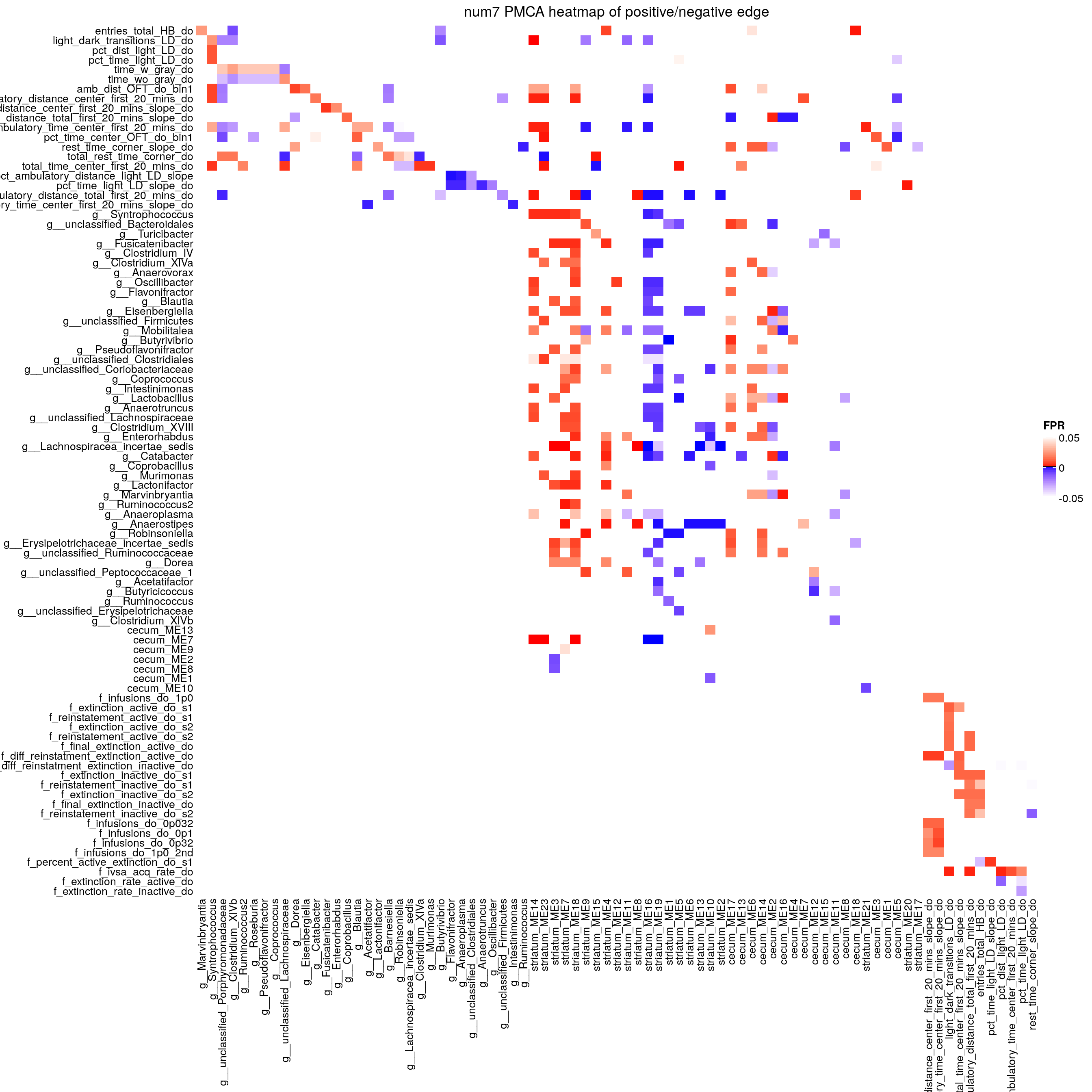
| Version | Author | Date |
|---|---|---|
| f7325c7 | xhyuo | 2025-01-15 |
load("data/Data_repository_Bubier/DO_predisposing_behaviors_domain.RData")
edges =  edgelist_all7
nodes <- data.frame(name = unique(c(edges$xname, edges$yname))) %>%
  dplyr::left_join(DO_predisposing_behaviors_domain, by = c("name" = "trait")) %>%
  dplyr::mutate(domain = case_when(
    str_detect(name, "cecum") ~ "cecum",
    str_detect(name, "striatum") ~ "striatum",
    str_detect(name, "f_") ~ "ivsa",
    str_detect(name, "g__") ~ "microbe",
    TRUE ~ as.character(domain)
  ))

edges_sankey <- data.frame(
  source = match(edges$xname, nodes$name) - 1,
  target = match(edges$yname, nodes$name) - 1,
  value = edges$fpr
  )

# Plot Sankey diagram
sankeyNetwork(Links = edges_sankey,
              Nodes = nodes,
              Source = "source",
              Target = "target",
              Value = "value",
              NodeID = "name",
              fontSize = 12,
              nodeWidth = 12,
              NodeGroup = "domain")
sessionInfo()
# R version 4.0.3 (2020-10-10)
# Platform: x86_64-pc-linux-gnu (64-bit)
# Running under: Ubuntu 20.04.2 LTS
#
# Matrix products: default
# BLAS/LAPACK: /usr/lib/x86_64-linux-gnu/openblas-pthread/libopenblasp-r0.3.8.so
#
# locale:
#  [1] LC_CTYPE=en_US.UTF-8       LC_NUMERIC=C
#  [3] LC_TIME=en_US.UTF-8        LC_COLLATE=en_US.UTF-8
#  [5] LC_MONETARY=en_US.UTF-8    LC_MESSAGES=C
#  [7] LC_PAPER=en_US.UTF-8       LC_NAME=C
#  [9] LC_ADDRESS=C               LC_TELEPHONE=C
# [11] LC_MEASUREMENT=en_US.UTF-8 LC_IDENTIFICATION=C
#
# attached base packages:
# [1] grid      stats     graphics  grDevices utils     datasets  methods
# [8] base
#
# other attached packages:
#  [1] testthat_3.0.2        networkD3_0.4         igraph_1.2.6
#  [4] biomaRt_2.46.3        gplots_3.1.1          RColorBrewer_1.1-2
#  [7] Hmisc_4.4-2           Formula_1.2-4         survival_3.2-7
# [10] lattice_0.20-41       circlize_0.4.12       WGCNA_1.72-5
# [13] fastcluster_1.1.25    dynamicTreeCut_1.63-1 PMCA_0.1.0
# [16] qtl2_0.24             forcats_0.5.1         stringr_1.4.0
# [19] dplyr_1.0.4           purrr_0.3.4           readr_1.4.0
# [22] tidyr_1.1.2           tibble_3.0.6          ggplot2_3.3.3
# [25] tidyverse_1.3.0       ComplexHeatmap_2.6.2  workflowr_1.6.2
#
# loaded via a namespace (and not attached):
#   [1] readxl_1.3.1          backports_1.2.1       BiocFileCache_1.14.0
#   [4] splines_4.0.3         crosstalk_1.1.1       digest_0.6.27
#   [7] foreach_1.5.1         htmltools_0.5.1.1     GO.db_3.12.1
#  [10] magrittr_2.0.1        checkmate_2.0.0       memoise_2.0.0
#  [13] cluster_2.1.0         doParallel_1.0.16     modelr_0.1.8
#  [16] matrixStats_0.58.0    askpass_1.1           prettyunits_1.1.1
#  [19] jpeg_0.1-8.1          colorspace_2.0-0      blob_1.2.1
#  [22] rvest_0.3.6           rappdirs_0.3.3        haven_2.3.1
#  [25] xfun_0.21             crayon_1.4.1          jsonlite_1.7.2
#  [28] impute_1.64.0         iterators_1.0.13      glue_1.4.2
#  [31] gtable_0.3.0          GetoptLong_1.0.5      shape_1.4.5
#  [34] BiocGenerics_0.36.1   scales_1.1.1          DBI_1.1.1
#  [37] Rcpp_1.0.6            progress_1.2.2        htmlTable_2.1.0
#  [40] clue_0.3-58           foreign_0.8-80        bit_4.0.4
#  [43] preprocessCore_1.52.1 DT_0.17               stats4_4.0.3
#  [46] htmlwidgets_1.5.3     httr_1.4.2            ellipsis_0.3.1
#  [49] pkgconfig_2.0.3       XML_3.99-0.5          nnet_7.3-14
#  [52] dbplyr_2.1.0          tidyselect_1.1.0      rlang_0.4.10
#  [55] later_1.1.0.1         AnnotationDbi_1.52.0  munsell_0.5.0
#  [58] cellranger_1.1.0      tools_4.0.3           cachem_1.0.4
#  [61] cli_2.3.0             generics_0.1.0        RSQLite_2.2.3
#  [64] broom_0.7.4           evaluate_0.14         fastmap_1.1.0
#  [67] yaml_2.2.1            knitr_1.31            bit64_4.0.5
#  [70] fs_1.5.0              caTools_1.18.1        whisker_0.4
#  [73] xml2_1.3.2            compiler_4.0.3        rstudioapi_0.13
#  [76] curl_4.3              png_0.1-7             reprex_1.0.0
#  [79] stringi_1.5.3         highr_0.8             desc_1.2.0
#  [82] Matrix_1.2-18         vctrs_0.3.6           pillar_1.4.7
#  [85] lifecycle_1.0.0       GlobalOptions_0.1.2   data.table_1.13.6
#  [88] bitops_1.0-6          httpuv_1.5.5          R6_2.5.0
#  [91] latticeExtra_0.6-29   promises_1.2.0.1      KernSmooth_2.23-17
#  [94] gridExtra_2.3         IRanges_2.24.1        codetools_0.2-16
#  [97] gtools_3.8.2          assertthat_0.2.1      pkgload_1.1.0
# [100] openssl_1.4.3         rprojroot_2.0.2       rjson_0.2.20
# [103] withr_2.4.1           S4Vectors_0.28.1      parallel_4.0.3
# [106] hms_1.0.0             rpart_4.1-15          rmarkdown_2.6
# [109] Cairo_1.5-12.2        git2r_0.28.0          Biobase_2.50.0
# [112] lubridate_1.7.9.2     base64enc_0.1-3
This R Markdown site was created with workflowr